... is also unclear how we can make a trade-off between the model precision and expected accuracy with these methods. arXiv:1706.02021v1 [cs.NE] 7 Jun 2017 ...
Network Sketching: Exploiting Binary Structure in Deep CNNs Yiwen Guo1 , Anbang Yao1 , Hao Zhao2,1 , Yurong Chen1 1 Intel Labs China, 2 Department of Electronic Engineering, Tsinghua University
arXiv:1706.02021v1 [cs.NE] 7 Jun 2017
{yiwen.guo,anbang.yao,hao.zhao,yurong.chen}@intel.com
Abstract Convolutional neural networks (CNNs) with deep architectures have substantially advanced the state-of-the-art in computer vision tasks. However, deep networks are typically resource-intensive and thus difficult to be deployed on mobile devices. Recently, CNNs with binary weights have shown compelling efficiency to the community, whereas the accuracy of such models is usually unsatisfactory in practice. In this paper, we introduce network sketching as a novel technique of pursuing binary-weight CNNs, targeting at more faithful inference and better trade-off for practical applications. Our basic idea is to exploit binary structure directly in pre-trained filter banks and produce binaryweight models via tensor expansion. The whole process can be treated as a coarse-to-fine model approximation, akin to the pencil drawing steps of outlining and shading. To further speedup the generated models, namely the sketches, we also propose an associative implementation of binary tensor convolutions. Experimental results demonstrate that a proper sketch of AlexNet (or ResNet) outperforms the existing binary-weight models by large margins on the ImageNet large scale classification task, while the committed memory for network parameters only exceeds a little.
1. Introduction Over the past decade, convolutional neural networks (CNNs) have been accepted as the core of many computer vision solutions. Deep models trained on a massive amount of data have delivered impressive accuracy on a variety of tasks, including but not limited to semantic segmentation, face recognition, object detection and recognition. In spite of the successes, mobile devices cannot take much advantage of these models, mainly due to their inadequacy of computational resources. As is known to all, camera based games are dazzling to be operated with object recognition and detection techniques, hence it is eagerly anticipated to deploy advanced CNNs (e.g., AlexNet [15], VGG-Net [25] and ResNet [10]) on tablets and smartphones. Nevertheless, as the winner of ILSVRC-2012 com-
Figure 1. Sketching a network model by exploiting binary structure within pre-trained filter banks, after which the full-precision model can be converted to an efficient one with binary (in black and light grey) connections.
petition, AlexNet comes along with nearly 61 million realvalued parameters and 1.5 billion floating-point operations (FLOPs) to classify an image, making it resource-intensive in different aspects. Running it for real-time applications would require considerable high CPU/GPU workloads and memory footprints, which is prohibitive on typical mobile devices. The similar situation occurs on the deeper networks like VGG-Net and ResNet. Recently, CNNs with binary weights are designed to resolve this problem. By forcing the connection weights to only two possible values (normally +1 and −1), researchers attempt to eliminate the required floating-point multiplications (FMULs) for network inference, as they are considered to be the most expensive operations. In addition, since the real-valued weights are converted to be binary, these networks would commit much less space for storing their parameters, which leads to a great saving in the memory footprints and thus energy costs [8]. Several methods have been proposed to train such networks [1, 2, 22]. However, the reported accuracy of obtained models is unsatisfactory on large dataset (e.g., ImageNet) [22]. Even worse, since straightforwardly widen the networks does not guarantee any increase in accuracy [14], it is also unclear how we can make a trade-off between the model precision and expected accuracy with these methods.
In this paper, we introduce network sketching as a new way of pursuing binary-weight CNNs, where the binary structures are exploited in pre-trained models rather than being trained from scratch. To seek the possibility of yielding state-of-the-art models, we propose two theoretical grounded algorithms, making it possible to regulate the precision of sketching for more accurate inference. Moreover, to further improve the efficiency of generated models (a.k.a., sketches), we also propose an algorithm to associatively implement binary tensor convolutions, with which the required number of floating-point additions and subtractions (FADDs)1 is likewise reduced. Experimental results demonstrate that our method works extraordinarily well on both AlexNet and ResNet. That is, with a bit more FLOPs required and a little more memory space committed, the generated sketches outperform the existing binaryweight AlexNets and ResNets by large margins, producing near state-of-the-art recognition accuracy on the ImageNet dataset. The remainder of this paper is structured as follows. In Section 2, we briefly introduce the related works on CNN acceleration and compression. In Section 3, we highlight the motivation of our method and provide some theoretical analyses for its implementations. In Section 4, we introduce the associative implementation for binary tensor convolutions. At last, Section 5 experimentally demonstrates the efficacy of our method and Section 6 draws the conclusions.
appealing speedups (2× to 4×) with acceptable accuracy drop (≤ 1%). 2 Unlike the above mentioned ones, some research works regard memory saving as the top priority. To tackle the storage issue of deep networks, Gong et al. [6], Wu et al. [31] and Lin et al. [18] consider applying the quantization techniques to pre-trained CNNs, and trying to make network compressions with minor concessions on the inference accuracy. Another powerful category of methods in this scope is network pruning. Starting from the early work of LeCun et al’s [17] and Hassibi & Stork’s [9], pruning methods have delivered surprisingly good compressions on a range of CNNs, including some advanced ones like AlexNet and VGGnet [8, 26, 7]. In addition, due to the reduction in model complexity, a fair speedup can be observed as a byproduct. As a method for generating binary-weight CNNs, our network sketching is orthogonal to most of the existing compression and acceleration methods. For example, it can be jointly applied with low-rank based methods, by first decomposing the weight tensors into low-rank components and then sketching them. As for the cooperation with quantization-based methods, sketching first and conducting product quantization thereafter would be a good choice.
3. Network Sketching
The deployment problem of deep CNNs has become a concern for years. Efficient models can be learnt either from scratch or from pre-trained models. Generally, training from scratch demands strong integration of network architecture and training policy [18], and here we mainly discuss representative works on the latter strategy. Early works are usually hardware-specific. Not restricted to CNNs, Vanhoucke et al. [28] take advantage of programmatic optimizations to produce a 3× speedup on x86 CPUs. On the other hand, Mathieu et al. [20] perform fast Fourier transform (FFT) on GPUs and propose to compute convolutions efficiently in the frequency domain. Additionally, Vasilache et al. [29] introduce two new FFTbased implementations for more significant speedups. More recently, low-rank based matrix (or tensor) decomposition has been used as an alternative way to accomplish this task. Mainly inspired by the seminal works from Denil et al. [4] and Rigamonti et al. [23], low-rank based methods attempt to exploit parameter redundancy among different feature channels and filters. By properly decomposing pretrained filters, these methods [5, 12, 16, 32, 19] can achieve
In general, convolutional layers and fully-connected layers are the most resource-hungry components in deep CNNs. Fortunately, both of them are considered to be overparameterized [4, 30]. In this section, we highlight the motivation of our method and present its implementation details on the convolutional layers as an example. Fullyconnected layers can be operated in a similar way. Suppose that the learnable weights of a convolutional layer L can be arranged and represented as {W(i) : 0 ≤ i < n}, in which n indicates the target number of feature maps, and W(i) ∈ Rc×w×h is the weight tensor of its ith filter. Storing all these weights would require 32 × c × w × h × n bit memory, and the direct implementation of convolutions would require s × c × w × h × n FMULs (along with the same number of FADDs), in which s indicates the spatial size of target feature maps. Since many convolutional models are believed to be informational redundant, it is possible to seek their lowprecision and compact counterparts for better efficiency. With this in mind, we consider exploiting binary structures within L, by using the divide and conquer strategy. We shall first approximate the pre-trained filters with a linear span of certain binary basis, and then group the identical basis tensors to pursue the maximal network efficiency. Details
1 Without ambiguity, we collectively abbreviate floating-point additions and floating-point subtractions as FADDs.
2 Some other works concentrate on learning low-rank filters from scratch [27, 11], which is out of the scope of our paper.
2. Related Works
are described in the following two subsections, in which we drop superscript (i) from W because the arguments apply to all the n weight tensors.
3.1. Approximating the Filters As claimed above, our first goal is to find a binary expansion of W that approximates it well (as P illustrated in m−1 Figure 2), which means W ≈ hB, ai = j=0 aj Bj , c×w×h×m in which B ∈ {+1, −1} and a ∈ Rm are the concatenations of m binary tensors {B0 , ..., Bm−1 } and the same number of scale factors {a0 , ..., am−1 }, respectively. We herein investigate the appropriate choice of B and a with a fixed m. Two theoretical grounded algorithms are proposed in Section 3.1.1 and 3.1.2, respectively.
Figure 2. Approximate the real-valued weight tensor with a sum of scaled binary tensors.
Algorithm 1 The direct approximation algorithm: Input: W: the pre-trained weight tensor, m: the desired cardinality of binary basis. Output: {Bj , aj : 0 ≤ j < m}: a binary basis and a series of scale factors. ˆ j ← W. Initialize j ← 0 and W repeat Calculate Bj and aj by Equation (3). ˆ j+1 = W ˆ j −aj Bj and update j ← j +1. Calculate W until j reaches its maximal number m.
under this circumstance, in which function sgn(·) calculates the element-wise sign of the input tensor, and t = c×w ×h. The above algorithm is summarized in Algorithm 1. It is considered to be heuristic (or greedy) in the sense that each Bj is selected to be the current optimum, regardless of whether it will preclude better approximations later on. Furthermore, some simple deductions give the following theoretical result. Theorem 1. For any m ≥ 0, Algorithm 1 achieves a reconstruction error e2 satisfying e2 ≤ kWk2 (1 − 1/t)m .
3.1.1
Direct Approximation
For easy understanding, we shall first introduce the direct approximation algorithm. Generally, the reconstruction error (or approximation error, round-off error) e2 := kW − hB, aik2 should be minimized to retain the model accuracy after expansion. However, as a concrete decision problem, directly minimizing e2 seems NP-hard and thus solving it can be very time consuming [3]. In order to finish up in reasonable time, we propose a heuristic algorithm, in which Bj and aj are sequentially learnt and each of them is selected to be the current optimum with respect to the e2 minimization criterion. That is,
2
ˆ
Bj , aj = arg min W − aB (1)
, j B∈B, a∈R
in which B := {+1, −1}c×w×h , the norm operator k · k is defined as kXk := hX, Xi1/2 for any 3-D tensor X, and ˆ j indicates the approximation residue after combining all W ˆj =W the previously generated tensor(s). In particular, W if j = 0, and j−1 X ˆ Wj = W − ak Bk (2) k=0
if j ≥ 1. It can be easily known that, through derivative calculations, Equation (1) is equivalent with ˆ j) Bj = sgn(W
and aj =
ˆ ji hBj , W t
(3)
(4)
ˆ j ), we can obtain that, Proof. Since Bj = sgn(W X (l) ˆ ji = ˆ j k, hBj , W |w ˆj | ≥ kW l
(5)
ˆ j , with superscript (l) indicates in which w ˆj is an entry of W its index. From Equation (2) and (5), we have ˆ j+1 k2 = kW ˆ j k2 − aj hBj , W ˆ ji kW ˆ j k2 = kW
ˆ j i2 hBj , W 1− ˆ j k2 tkW
! (6)
ˆ j k2 (1 − 1/t) . ≤ kW The result follows by applying Formula (6) for j varying from 0 to m − 1. 3.1.2
Approximation with Refinement
We can see from Theorem 1 that, by utilizing the direct approximation algorithm, the reconstruction error e2 decays exponentially with a rate proportional to 1/t. That is, given a W with small size (i.e., when t is small), the approximation in Algorithm 1 can be pretty good with only a handful of binary tensors. Nevertheless, when t is relatively large, the reconstruction error will decrease slowly and the approximation can be unsatisfactory even with a large number of binary tensors. In this section, we propose to refine the direct approximation algorithm for better reconstruction property.
Algorithm 2 Approximation with refinement: Input: W: the pre-trained weight tensor, m: the desired cardinality of binary basis. Output: {Bj , aj : 0 ≤ j < m}: a binary basis and a series of scale factors. ˆ j ← W. Initialize j ← 0 and W repeat Calculate Bj and aj by Equation (3) and (7). ˆ j by Equation (2). Update j ← j + 1 and calculate W until j reaches its maximal number m.
Considering that, in Algorithm 1, both Bj and aj are chosen to minimize e2 with fixed counterparts. However, in most cases, it is doubtful whether B and a are optimal overall. If not, we may need to refine at least one of them for the sake of better approximation. On account of the computational simplicity, we turn to a specific case when B is fixed. That is, suppose the direct approximation has ˆ and a ˆ, we hereby seek another scale already produced B ˆ aik2 ≤ kW − hB, ˆ a ˆik2 . To vector a satisfying kW − hB, achieve this, we follow the least square regression method and get �−1 T aj = BjT Bj Bj · vec(W), (7) in which the operator vec(·) gets a column vector whose elements are taken from the input tensor, and Bj gets [vec(B0 ), ..., vec(Bj )]. The above algorithm with scale factor refinement is summarized in Algorithm 2. Intuitively, the refinement operation attributes a memory-like feature to our method, and the following theorem ensures it can converge faster in comparison with Algorithm 1. Theorem 2. For any m ≥ 0, Algorithm 2 achieves a reconstruction error e2 satisfying 2
e ≤ kWk
2
m−1 Y� j=0
1 1− t − λ(j, t)
� ,
(8)
in which λ(j, t) ≥ 0, for 0 ≤ j ≤ m − 1. Proof. To simplify the notations, let us further denote wj := vec(Wj ) and bj+1 := vec(Bj+1 ), then we can obtain by block matrix multiplication and inverse that, � � Φ + Φψψ T Φ/r −Φψ/r T −1 (Bj+1 Bj+1 ) = , (9) −ψ T Φ/r 1/r in which Φ = (BjT Bj )−1 , ψ = BjT bj+1 , and r = bTj+1 bj+1 − ψ T Φψ. Consequently, we have the following equation for j = 0, ..., m − 1, ! Λ(bj+1 bTj+1 ) wj+1 = I − T wj , (10) bj+1 Λbj+1
by defining Λ := I − Bj ΦBjT . As we know, given positive semi-definite matrices X and Y , tr(XY ) ≤ tr(X)tr(Y ). Then, Equation (10) gives, ˆ j+1 k2 ≤ kW ˆ j k2 − kW ˆ j k2 − = kW ˆ jk = kW
2
wjT (bj+1 bTj+1 )Λ(bj+1 bTj+1 )wj (bTj+1 Λbj+1 )2 wjT (bj+1 bTj+1 )wj bTj+1 Λbj+1
1−
ˆ j i2 hBj , W ˆ j k2 Λbj+1 kW
bTj+1
! .
Obviously, it follows that, ˆ j+1 k2 ≤ kW ˆ j k2 (1 − 1/(t − λ(j, t))), kW
(11)
in which λ(j, t) := bTj+1 (I − Λ)bj+1 . Since λ(j, t) represents the squared Euclidean norm of an orthogonal projection of bj+1 , it is not difficult to prove λ(j, t) ≥ 0, and then the result follows.
3.2. Geometric Interpretation After expanding the pre-trained filters, we can group the identical binary tensors to save some more memory footprints. In this paper, the whole technique is named as network sketching, and the generated binary-weight model is straightforwardly called a sketch. Next we shall interpret the sketching process from a geometric point of view. For a start, we should be aware that, Equation (1) is essentially seeking a linear subspace spanned by a set of t-dimensional binary vectors to minimize its Euclidean distance to vec(W). In concept, there are two variables to be determined in this problem. Both Algorithm 1 and 2 solve it in a heuristic way, and the jth binary vector is always estimated by minimizing the distance between itself and the current approximation residue. What make them different is that, Algorithm 2 takes advantage of the linear span of its previous j−1 estimations for better approximation, whereas Algorithm 1 does not. Let us now take a closer look at Theorem 2. Compared with Equation (4) in Theorem 1, the distinction of Equation (8) mainly lies in the existence of λ(j, t). Clearly, Algorithm 2 will converge faster than Algorithm 1 as long as λ(j, t) > 0 holds for any j ∈ [0, m − 1]. Geometrically speaking, if we consider Bj (BjT Bj )−1 BjT as the matrix of an orthogonal projection onto Sj := span(b0 , ..., bj ), then λ(j, t) is equal to the squared Euclidean norm of a vector projection. Therefore, λ(j, t) = 0 holds if and only if vector bj+1 is orthogonal to Sj , or in other words, orthogonal to each element of {b0 , ..., bj } which occurs with extremely low probability and only on the condition of t ∈ {2k : k ∈ N}. That is, Algorithm 2 will probably prevail over Algorithm 1 in practice.
4. Speeding-up the Sketch Model Using Algorithm 1 or 2, one can easily get a set of mn binary tensors on L, which means the storage requirement of learnable weights is reduced by a factor of 32t/(32m + tm)×. When applying the model, the required number of FMULs is also significantly reduced, by a factor of (t/m)×. Probably, the only side effect of sketching is some increases in the number of FADDs, as it poses an extra burden on the computing units. In this section, we try to ameliorate this defect and introduce an algorithm to further speedup the binary-weight networks. We start from an observation that, yet the required number of FADDs grows monotonously with m, the inherent number of addends and augends is always fixed with a given input of L. That is, some repetitive FADDs exist in the direct implementation of binary tensor convolutions. Let us denote X ∈ Rc×w×h as an input sub-feature map and see Figure 3 for a schematic illustration.
Bj1 +1 +1 −1 −1
Bj2 −1 +1 −1 +1
Bj1 ∨ Bj2 −1 0 0 +1
Table 1. Truth table of the element-wise operator ∨.
Since Bj0 Y Bj1 produces ternary outputs on each index position, we can naturally regard X ∗ (Bj0 Y Bj1 ) as an iteration of switch ... case ... statements. In this manner, only the entries corresponding to ±1 in Bj0 YBj1 need to be operated in X, and thus acceleration is gained. Assuming that the inner-product of Bj0 and Bj1 equals to r, then (t − r)/2 + 1 and (t + r)/2 + 1 FADDs are still required for calculating Equation (12) and (13), respectively. Obviously, we expect the real number r ∈ [−t, +t] to be close to either t or −t for the possibility of fewer FADDs, and thus faster convolutions in our implementation. In particular, if r ≥ 0, Equation (12) is chosen for better efficiency; otherwise, Equation (13) should be chosen.
4.2. Constructing a Dependency Tree
Figure 3. As highlighted in the rounded rectangles, with high probability, repetitive FADD exists in the direct implementation of binary tensor convolutions.
4.1. Associative Implementation To properly avoid redundant operations, we first present an associative implementation of the multiple convolutions X ∗ B0 , ..., X ∗ Bmn−1 on L, in which the connection among different convolutions is fully exploited. To be more specific, our strategy is to perform convolutions in a hierarchical and progressive way. That is, each of the convolution results is used as a baseline of the following calculations. Suppose the j0 -th convolution is calculated in advance and it produces X∗Bj0 = s, then the convolution of X and Bj1 can be derived by using X ∗ Bj1 = s + (X ∗ (Bj0 Y Bj1 )) × 2,
(12)
or alternatively, X ∗ Bj1 = s − (X ∗ (¬Bj0 Y Bj1 )) × 2,
(13)
in which ¬ denotes the element-wise not operator, and Y denotes an element-wise operator whose behavior is in accordance with Table 1.
Our implementation works by properly rearranging the binary tensors and implementing binary tensor convolutions in an indirect way. For this reason, along with Equations (12) and (13), a dependency tree is also required to drive it. In particular, dependency is the notion that certain binary tensors are linked to specify which convolution to perform first and which follows up. For instance, with the depth-first-search strategy, T in Figure 4 shows a dependency tree indicating first to calculate X∗B1 , then to derive X ∗ B0 from the previous result, then to calculate X ∗ B3 on the base of X ∗ B0 , and so forth. By traversing the whole tree, all mn convolutions will be progressively and efficiently calculated.
Figure 4. A dependency tree for our algorithm. It suggests an order under which the associative convolutions are to be performed.
In fact, our algorithm works with a stochastically given tree, but a dedicated T is still in demand for its optimum performance. Let G = {V, E} be an undirected weighted graph with the vertex set V and weight matrix E ∈ Rmn×mn . Each element of V represents a single binary tensor, and each element of E measures the distance
Algorithm 3 The associative implementation: Input: {Bj : 0 ≤ j < mn}: the set of binary tensors, X: the input sub-feature map, T : the dependency tree. Output: {yj : 0 ≤ j < mn}: the results of convolution. Get z = T .root and calculate yz.key = X ∗ Bz.key . Initialize the baseline value by s ← yz.key . repeat Search the next node of T and update z, s. Calculate yz.key by using Equation (12) or (13). until search ends. between two chosen tensors. To keep in line with the previous subsection, we here define the distance function of the following form � � t+r t−r , , (14) d(Bj0 , Bj1 ) := min 2 2 in which r = hBj0 , Bj1 i indicates the inner-product of Bj0 and Bj1 . Clearly, the defined function is a metric on {−1, +1}c×w×h and its range is restricted in [0, t]. Recall that, we expect r to be close to ±t in the previous subsection. In consequence, the optimal dependency tree should have the shortest distance from root to each of its vertices, and thus the minimum spanning tree (MST) of G is what we want. From this perspective, we can use some off-the-shell algorithms to construct such a tree. Prim’s algorithm [21] is chosen in this paper on account of its linear time complexity with respect to |E|, i.e., O(m2 n2 ) on L. With the obtained T , one can implement our algorithm easily and the whole process is summarized in Algorithm 3. Note that, although the fully-connected layers calculate vector-matrix multiplications, they can be considered as a bunch of tensor convolutions. Therefore, in the binary case, we can also make accelerations in the fully-connected layers by using Algorithm 3.
5. Experimental Results In this section, we try to empirically analyze the proposed algorithms. For pragmatic reasons, all experiments are conducted on the famous ImageNet ILSVRC-2012 database [24] with advanced CNNs and the open-source Caffe framework [13]. The training set is comprised of 1.2 million labeled images and the test set is comprised of 50,000 validation images. In Section 5.1 and 5.2, we will test the performance of the sketching algorithms (i.e., Algorithm 1 and 2) and the associative implementation of convolutions (i.e., Algorithm 3) in the sense of filter approximation and computational efficiency, respectively. Then, in Section 5.3, we evaluate the whole-net performance of our sketches and compare them with other binary-weight models.
Layer Name Conv1 Conv2 Conv3 Conv4 Conv5 Fc6 Fc7 Fc8
Filters 96 256 384 384 256 1 1 1
Params (b) ∼1M ∼10M ∼28M ∼21M ∼14M ∼1208M ∼537M ∼131M
FLOPs ∼211M ∼448M ∼299M ∼224M ∼150M ∼75M ∼34M ∼8M
Table 2. Details of the learnable layers in AlexNet [15], in which ”Conv2” is the most computationally expensive one and ”Fc6” commits the most memory (in bits). In all these layers, FLOPs consist of the same number of FADDs and FMULs.
5.1. Efficacy of Sketching Algorithms As a starting experiment, we consider sketching the famous AlexNet model [15]. Although it is the champion solution of ILSVRC-2012, AlexNet seems to be very resource-intensive. Therefore, it is indeed appealing to seek its low-precision and efficient counterparts. As claimed in Section 1, AlexNet is an 8-layer model with 61M learnable parameters. Layer-wise details are shown in Table 2, and the pre-trained reference model is available online 3 . Using Algorithm 1 and 2, we are able to generate binaryweight AlexNets with different precisions. Theoretical analyses have been given in Section 3, so in this subsection, we shall empirically analyze the proposed algorithms. In particular, we demonstrate in Figure 6 how ”energy” accumulates with a varying size of memory P commitment for P different approximators. Defined as 1 − e2 / kW k2 , the accumulative energy is negatively correlated with reconstruction error [32], so the faster it increases, the better. In the figure, our two algorithms are abbreviately named as ”Sketching (direct)” and ”Sketching (refined)”. To compare with other strategies, we also test the stochastically generated binary basis (named ”Sketching random”) as used in [14], and the network pruning technique [8] which is not naturally orthogonal with our sketching method. The scalar factors for ”Sketching (random)” is calculated by Equation (7) to ensure its optimal performance. We can see that, it is consistent with the theoretical result that Algorithm 1 converges much slower than Algorithm 2 on all learnable layers, making it less effective on the filter approximation task. However, on the other hand, Algorithm 1 can be better when compared with ”Sketching (random)” and the pruning technique. With small working memory, our direct approximation algorithm approximates better. However, if the memory size increases, pruning technique may converge faster to its optimum. 3 https://github.com/BVLC/caffe/tree/master/ models/bvlc_alexnet.
As discussed in Section 4, parameter m balances the model accuracy and efficiency in our algorithms. Figure 6 shows that, a small m (for example 3) should be adequate for AlexNet to attain over 80% of the accumulative energy in its refined sketch. Let us take layer ”Conv5” and ”Fc6” as examples and see Table 3 for more details. Layer Name Conv2 sketch Fc6 sketch
Energy (%) 82.9 94.0
Params (b) ∼0.9M ∼114M
FMULs ∼560K ∼12K
Table 3. With only 3 bits allocated, the refined sketch of AlexNet attains over 80% of the energy on ”Conv2” and ”Fc6”, and more than 10× reduction in the committed memory for network parameters. Meanwhile, the required number of FMULs is also extremely reduced (by 400× and ∼3000×) on the two layers.
5.2. Efficiency of Associative Manipulations The associative implementation of binary tensor manipulations (i.e., Algorithm 3) is directly tested on the 3-bit refined sketch of AlexNet. To begin with, we still focus on ”Conv2 sketch” and ”Fc6 sketch”. Just to be clear, we produce the result of Algorithm 3 with both a stochastically generated dependency tree and a delicately calculated MST, while the direct implementation results are compared as a benchmark. All the implementations require the same number of FMULs, as demonstrated in Table 3, and significantly different number of FADDs, as compared in Table 4. Note that, in the associative implementations, some logical evaluations and ×2 operations are specially involved. Nevertheless, they are much less expensive than the FADDs and FMULs [22], by at least an order of magnitude. Hence, their cost are not deeply analyzed in this subsection 4 . Implementation Direct Associative (random) Associative (MST)
Conv2 sketch ∼672M ∼328M ∼265M
Fc6 sketch ∼113M ∼56M ∼49M
Table 4. The associative implementation remarkably reduces the required number of FADDs on ”Conv2 sketch” and ”Fc6 sketch”.
From the above table, we know that our associative implementation largely reduces the required number of FADDs on ”Conv2 sketch” and ”Fc6 sketch”. That is, it properly ameliorates the adverse effect of network sketching and enables us to evaluate the 3-bit sketch of AlexNet without any unbearably increase in the required amount of computation. In addition, the MST helps to further improve its performance and finally get ∼2.5× and ∼ 2.3× reduc4 Since the actual speedups varies dramatically with the architecture of processing units, so we will not measure it in the paper.
Figure 5. The associative implementation of binary tensor convolutions helps to gain 2× to 3× reductions in the required number of FADDs on all learnable layers of ”AlexNet sketch”.
tions on the two layers respectively. Results on all learnable layers are summarized in Figure 5.
5.3. Whole-net Performance Having tested Algorithm 1, 2 and 3 on the base of their own criteria, it is time to compare the whole-net performance of our sketch with that of other binary weight models [1, 22]. Inspired by the previous experimental results, we still use the 3-bit (direct and refined) sketches for evaluation, as they are both very efficient and accurate. Considering that the fully-connected layers of AlexNet contain more than 95% of its parameters, we should try sketching them to an extreme, namely 1 bit. Similar with Rastegari et al. [22], we also keep the ’fc8’ layer (or say, the output layer) to be of its full precision and report the top-1 and top5 inference accuracies. However, distinguished from their methods, we sketch the ’conv1’ layer as well because it is also compute-intensive (as shown in Table 1). Model Reference Sketch (ref.) Sketch (dir.) BWN [22] BC [1]
Params (b) ∼1951M ∼193M ∼193M ∼190M ∼189M
Top-1 (%) 57.2 55.2 54.4 53.8 35.4
Top-5 (%) 80.3 78.8 78.1 77.0 61.0
Table 5. Network sketching technique generates binary-weight AlexNets with the ability to make faithful inference and roughly 10.1× fewer parameters than its reference (in bits). Test accuracies of the competitors are cited from the paper. An updated version of BWN gains significantly improved accuracies (top-1: 56.8% and top-5: 79.4%), but the technical improvement seems unclear.
Just to avoid the propagation of reconstruction errors, we need to somehow fine-tune the generated sketches. Naturally, there are two protocols to help accomplish this task; one is known as projection gradient descent and the other is stochastic gradient descent with full precision weight update [1]. We choose the latter by virtue of its better convergency. The training batch size is set as 256 and the momentum is 0.9. We let the learning rate drops every 20,000 iterations from 0.001, which is one tenth of the original
Figure 6. Network sketching approximates AlexNet well enough with a much smaller amount of committed memory, and the refinement operation helps to achieve better convergency on all of its learnable layers.
value as set in Krizhevsky et al.’s paper [15], and use only the center crop for accuracy evaluation. After totally 70,000 iterations (i.e., roughly 14 epochs), our sketches can make faithful inference on the test set, and the refined model is better than the direct one. As shown in Table 5, our refined sketch of AlexNet achieves a top-1 accuracy of 55.2% and a top-5 accuracy of 78.8%, which means it outperforms the recent released models in the name of BinaryConnect (BC) [1] and Binary-Weight Network (BWN) [22] by large margins, while the required number of parameters only exceeds a little bit. Network pruning technique also achieves compelling results on compressing AlexNet. However, it demands a lot of extra space for storing parameter indices, and more importantly, even the optimal pruning methods perform mediocrely on convolutional layers [8, 7]. In contrast, network sketching works sufficiently well on both of the layer types. Here we also testify its efficacy on ResNet [10]. Being equipped with much more convolutional layers than that of AlexNet, ResNet wins the ILSVRC-2015 classification competition. There are many instantiations of its architecture, and for fair comparisons, we choose the type B version of 18 layers (as with Rastegari et al. [22]). A pre-trained Torch model is available online 5 and we convert it into an equivalent Caffe model before sketching 6 . For the fine-tuning process, we set the training batch size as 64 and let the learning rate drops from 0.0001. After 200,000 iterations (i.e., roughly 10 epochs), the generated 5 https://github.com/facebook/fb.resnet.torch/ tree/master/pretrained. 6 https://github.com/facebook/fb-caffe-exts.
sketch represents a top-1 accuracy of 67.8% and a top-5 accuracy of 88.4% on ImageNet dataset. Refer to Table 6 for a comparison of the classification accuracy of different binary-weight models. Model Reference Sketch (ref.) Sketch (dir.) BWN [22]
Params (b) ∼374M ∼51M ∼51M ∼28M
Top-1 (%) 68.8 67.8 67.3 60.8
Top-5 (%) 89.0 88.4 88.2 83.0
Table 6. Network sketching technique generates binary-weight ResNets with the ability to make faithful inference and roughly 7.4× fewer parameters than its reference (in bits). The test accuracies of BWN are directly cited from its paper.
6. Conclusions In this paper, we introduce network sketching as a novel technology for pursuing binary-weight CNNs. It is more flexible than the current available methods and it enables researchers and engineers to regulate the precision of generated sketches and get better trade-off between the model efficiency and accuracy. Both theoretical and empirical analyses have been given to validate its efficacy. Moreover, we also propose an associative implementation of binary tensor convolutions to further speedup the sketches. After all these efforts, we are able to generate binary-weight AlexNets and ResNets with the ability to make both efficient and faithful inference on the ImageNet classification task. Future works shall include exploring the sketching results of other CNNs.
References [1] M. Courbariaux, Y. Bengio, and J.-P. David. BinaryConnect: Training deep neural networks with binary weights during propagations. In Advances in Neural Information Processing Systems (NIPS), 2015. [2] M. Courbariaux, I. Hubara, D. Soudry, R. El-Yaniv, and Y. Bengio. Binarized neural networks: Training deep neural networks with weights and activations constrained to +1 or -1. In arXiv preprint arXiv:1602.02830, 2016. [3] G. Davis, S. Mallat, and M. Avellaneda. Adaptive greedy approximations. Constructive approximation, 13(1):57–98, 1997. [4] M. Denil, B. Shakibi, L. Dinh, M. Ranzato, and N. d. Freitas. Predicting parameters in deep learning. In Advances in Neural Information Processing Systems (NIPS), 2013. [5] E. L. Denton, W. Zaremba, J. Bruna, Y. LeCun, and R. Fergus. Exploiting linear structure within convolutional networks for efficient evaluation. In Advances in Neural Information Processing Systems (NIPS), 2014. [6] Y. Gong, L. Liu, M. Yang, and L. Bourdev. Compressing deep convolutional networks using vector quantization. arXiv preprint arXiv:1412.6115, 2014. [7] Y. Guo, A. Yao, and Y. Chen. Dynamic network surgery for efficient DNNs. In Advances in Neural Information Processing Systems (NIPS), 2016. [8] S. Han, J. Pool, J. Tran, and W. J. Dally. Learning both weights and connections for efficient neural networks. In Advances in Neural Information Processing Systems (NIPS), 2015. [9] B. Hassibi and D. G. Stork. Second order derivatives for network pruning: Optimal brain surgeon. In Advances in Neural Information Processing Systems (NIPS), 1993. [10] K. He, X. Zhang, S. Ren, and J. Sun. Deep residual learning for image recognition. In IEEE Conference on Computer Vision and Pattern Recognition (CVPR), 2016. [11] Y. Ioannou, D. Robertson, J. Shotton, R. Cipolla, and A. Criminisi. Training CNNs with low-rank filters for efficient image classification. In International Conference on Learning Representations (ICLR), 2016. [12] M. Jaderberg, A. Vedaldi, and A. Zisserman. Speeding up convolutional neural networks with low rank expansions. In British Machine Vision Conference (BMVC), 2014. [13] Y. Jia, E. Shelhamer, J. Donahue, S. Karayev, J. Long, R. Girshick, S. Guadarrama, and T. Darrell. Caffe: Convolutional architecture for fast feature embedding. In ACM Multimedia Conference (MM), 2014. [14] F. Juefei-Xu, V. N. Boddeti, and M. Savvides. Local binary convolutional neural networks. arXiv preprint arXiv:1608.06049, 2016. [15] A. Krizhevsky, I. Sutskever, and G. E. Hinton. Imagenet classification with deep convolutional neural networks. In Advances in neural information processing systems (NIPS), 2012. [16] V. Lebedev, Y. Ganin, M. Rakhuba, I. Oseledets, and V. Lempitsky. Speeding-up convolutional neural networks using fine-tuned CP-decomposition. arXiv preprint arXiv:1412.6553, 2014.
[17] Y. LeCun, J. S. Denker, S. A. Solla, R. E. Howard, and L. D. Jackel. Optimal brain damage. In Advances in Neural Information Processing Systems (NIPS), 1989. [18] D. D. Lin, S. S. Talathi, and V. S. Annapureddy. Fixed point quantization of deep convolutional networks. In International Conference on Machine Learning (ICML), 2016. [19] B. Liu, M. Wang, H. Foroosh, M. Tappen, and M. Pensky. Sparse convolutional neural networks. In IEEE Conference on Computer Vision and Pattern Recognition (CVPR), 2015. [20] M. Mathieu, M. Henaff, and Y. LeCun. Fast training of convolutional networks through FFTs. arXiv preprint arXiv:1312.5851, 2013. [21] R. C. Prim. Shortest connection networks and some generalizations. Bell system technical journal, 36(6):1389–1401, 1957. [22] M. Rastegari, V. Ordonez, J. Redmon, and A. Farhadi. XNOR-Net: Imagenet classification using binary convolutional neural networks. arXiv preprint arXiv:1603.05279v2, 2016. [23] R. Rigamonti, A. Sironi, V. Lepetit, and P. Fua. Learning separable filters. In IEEE Conference on Computer Vision and Pattern Recognition (CVPR), 2013. [24] O. Russakovsky, J. Deng, H. Su, J. Krause, S. Satheesh, S. Ma, Z. Huang, A. Karpathy, A. Khosla, M. Bernstein, A. C. Berg, and L. Fei-Fei. ImageNet Large Scale Visual Recognition Challenge. International Journal of Computer Vision (IJCV), 115(3):211–252, 2015. [25] K. Simonyan and A. Zisserman. Very deep convolutional networks for large-scale image recognition. In International Conference on Learning Representations (ICLR), 2014. [26] S. Srinivas and R. V. Babu. Data-free parameter pruning for deep neural networks. In British Machine Vision Conference (BMVC), 2015. [27] C. Tai, T. Xiao, Y. Zhang, X. Wang, and W. E. Convolutional neural networks with low-rank regularization. In International Conference on Learning Representations (ICLR), 2016. [28] V. Vanhoucke, A. Senior, and M. Z. Mao. Improving the speed of neural networks on CPUs. In Deep Learning and Unsupervised Feature Learning Workshop, Advances in Neural Information Processing Systems (NIPS Workshop), 2011. [29] N. Vasilache, J. Johnson, M. Mathieu, S. Chintala, S. Piantino, and Y. LeCun. Fast convolutional nets with fbfft: A GPU performance evaluation. In International Conference on Learning Representations (ICLR), 2015. [30] A. Veit, M. Wilber, and S. Belongie. Residual networks are exponential ensembles of relatively shallow networks. In Advances in Neural Information Processing Systems (NIPS), 2016. [31] J. Wu, C. Leng, Y. Wang, Q. Hu, and J. Cheng. Quantized convolutional neural networks for mobile devices. IEEE Conference on Computer Vision and Pattern Recognition (CVPR), 2016. [32] X. Zhang, J. Zou, X. Ming, K. He, and J. Sun. Efficient and accurate approximations of nonlinear convolutional networks. In IEEE Conference on Computer Vision and Pattern Recognition (CVPR), 2015.