Network Topology Optimization in Wireless Sensor ...

Network Topology Optimization in Wireless Sensor Networks in Precision Agriculture Katsalis Konstantinos, Xenakis Apostolos, Anta Sakellariou, Kikiras Panagiotis University Of Thessaly Department of Computer and Communications Engineering,Glavany 37 -28 October Street, 38331,Volos Magnesia {axenakis, kkatsalis, ansakell, kikirasp}@inf.uth.gr

ABSTRACT The objective of this paper is to explain how a typical WSN works, which are the pros and cons and the technical characteristics, as well as the financial benefits by applying sensor technology in the field. Furthermore a new method of network topology construction is proposed based on electrical conductivity and management zones. 1.

INTRODUCTION

Precision Agriculture refers to the use of an information system for the within-field management of crops. This basically means to add the right quantity of fertilizer to the right time and to the exact location within certain cultivate extend of ground [7]. In fact this means than every part of the crop is treated in different way and not as a whole part. The use of precision agriculture techniques gives agronomists the potential to apply new and continuously developing technologies which help to manage better the production. Some of these technologies are the GPS, GIS, Remote Sensing [5], Variable Rate Technology, Machine Controls and Smart Sensor Arrays and the WSN technology [6]. 2.

WIRELESS SENSOR NETWORKS

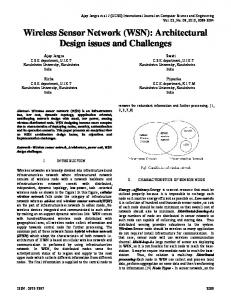
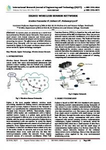
2.1 WSN technology A number of sensors which will be placed appropriately and will cover the whole filed are required for a WSN to function [8]. These sensors can be programmed to record measures like temperature and humidity. All the data which are collected from the sensors, using a wireless multi-hop routing technology, end up in a gateway which transfers them to the end user through wireless network, internet or LAN [4].

Figure 1 : A Wireless Sensor Network

2.2 The advantages from applying a WSN in the field The benefits which arise from the application of precision agriculture technique come up from the precision in the irrigation quantity, the use of chemurgy only in the appropriate field areas, the control in the quantities of the fertilizer, the exact definition of the semination and crop. More over the use of appropriate quality of seed depending on the field conditions, water control, the optimum quantity of seed semination and spending less money on agriculture scientists and consulting firms are factors that WSN has a direct impact. In addition with WSN the advantages [1],[2] are: o Ability to observe for long periods of time crop state. o Direct, exact briefing of the field state and ability to interfere in case of an emergency. o Distant decision making o Analytical information storage in order to create a case record of the field crop. o Friendly Graphical User Interface with the monitoring system. o Potential to make exact evaluation of new crop methods and techniques. 3. MATERIALS AND METHODS Precision Agriculture is mainly based on the management of the field’s differentiality. The differentiallity in the production is defined from the variability in the field structure, the organic matter, the level of saline and the level of water. In order to treat the field in different ways, detailed management field maps should be produced, on which this differentiallity is depicted. The production of these management maps give in an indirect way evidence of how the topological diagram of the WSN should be built. 3.1 Management Zones The field management zones are smaller parts of the field which show certain variability from each other and each of them needs different management treatment and tactics. The criterion to create the management zones is not only one and is not always fixed. The categorisation depends on several factors which the agronomists decide that are capable to do so, for example humidity, organic matter or agile. In figure 2 management zones are depicted, each of which have individual characteristics.

Figure 2: Management Zones 3.2 Electric conductivity and Veris System The Electric Conductivity is a measurement of easiness with which electric current goes through the soil. It mainly depends from the presence of salts and the constitution of soil in sand, clay, organic substance and water. Regions with the same EC values belong in the same territorial type with a great probability and thus management maps construction can be done based in EC measurements. According to so far research, the measurements of electrical conductivity are mainly influenced from humidity. This

means that each time the levels of humidity change within the field the network should not be re-designed because these levels change respectively for the entire field and the management zones remain the same as before and so the network diagram is not affected either. One of the most used systems for measurement of electric conductivity is Veris 3100. This device comes along with a GPS receptor so that each measurement is recorded precisely and collected in a central unit. A data file is produced for each area scanned with Veris including each measurement along with the coordinates of the point that the measurement was taken. The data can be represented in a graphic mode so that regions with similar characteristics can be categorized, distinguished and clearly seen. This requires processing of data from specialised software of geographic information system (GIS). 3.3 Topology efficiency The aforesaid approach is applied for the segregation of field in management areas, in order to avoid the node placement in grid topology. An appropriate number of sensors which will completely cover the informative needs from the aspect of data are placed so that a complete picture of the total field is drawn. The following methodology for the optimal placement of sensors is used: 1. Scanning of all extent with the system Veris 3100. 2. Explicit segregation between zones. 3. Registration of points in the field which can cause problem in communication. 4. Placement of nodes in points in which communication is achieved. In an existing field in which cotton is cultivated, in the region of Karditsa, with an extent of 50 acres, the aforesaid methodology is used in management zones that have been drawn by Veris, according to the work done by Athanasios Markinos, a Phd candidate in the Department of Agriculture Crop Production and Rural Environment of the University of Thessaly. Using Veris to scan in a depth of 90cm, the 50 acres field is segmented in five distinguishable zones. Simulations are done using the two following network topologies. A grid topology of 56 sensors with 32m vertical and horizontal distance each. A proposed methodology of 17 sensors with medium distance of 34,8m among sensors.

Figure 6: Grid Topology & Optimal nodes placement The coverage distance for each node depends on the node and RF technology. The nodes were not put at the maximum coverage distance for more power efficiency. The

medium distance of 35m results from distances of nodes, in which there is a high possibility of communication between them (the Signal – to – Noise ratio was above a certain threshold). Clearly there is a trade-off between the number of nodes used (lower cost in euros) and the network robustness. The reduction in the number of sensors that is reached in the cotton cultivation, reaches 70%. This ratio occurs when the absolutely necessary nodes are used to cover the management zones. In a more robust solution, some extra nodes are used which are placed in key communication positions in the field. A key point in the design of the network is to take under consideration factors such as scattering, the absorption and weakening of the signal that depend each time on the type of the cultivation, the height of leafage as also hillocks and pieces of machinery in the field, and lastly the sources of electric noise such as high voltage cables [7]. Other factors are still the technology of sensors used and real climatic conditions that prevail in the region. 4. SIMULATION RESULTS The simulation was done in Prowler, which is an event – based simulator, a framework based to TinyOS/NesC. Based on Prowler simulator, the base platform of the simulations which was used is Rmaze that provides a set of performance metrics for comparing different routing algorithms.The simulation time is calibrated to 100 seconds. Some definitions of the metrics are: Latency: Time to send a message from source to destination. For any destination, if n n di packets have arrived, latency for that destination is given by , where di is the 1 n latency of the ith packet. Network latency is then averaged by the number of destinations. Throughput: Number of messages per second received at destination. The throughput of the network is the sum of the throughputs from all destinations.

Figure 7: Network Latency – Network throughput Latency in veris case is much less that latency in grid topology. Generally we have calculated the average network latency throughout the simulation for the two cases which is 0.0842 for the grid and 0.038 for the veris. In veris latency is decreased by approximately 55%. We observe that in veris topology throughput is lower than that in grid, because in grid topology the total packets sent to the destination are much more that the packets sent by sources in the veris topology.

Success Rate: The total number of packets received at all the destinations vs. the total number of packets sent from all the sources. Loss Rate: Number of lost packets vs. the total expected number of packets for that destination. Energy consumption: Sum of used energy of all the nodes, where the used energy of a node is the sum of the energy used for communication, including transmitting (Pt), receiving (Pr) and idling (Pi).

Figure 8: Network Success Rate - Network Loss Rate In veris topology success rate for a long portion of simulation time is increasing. This means that more packets are likely to be delivered to the destination. Approximately after 60 seconds in veris topology the success rate is near 80%. On the contrary, in grid topology, we observe that not only success rate is on average constant, but it has converged approximately to 40%. The maximum difference in success rate measurements in both topologies reaches about 50%. In our optimized veris topology loss rate is much less than that in grid topology. We also observe that in veris topology the graph of loss rate is decreasing throughout simulation time. 5. FINANCIAL BENEFITS 5.1 How Precision Agriculture affects cultivation The following table summarizes all the measurements that is taken by Precision Agriculture methods and depicts which cultivation factors every measurement influences: Table 1. measurements that is taken by Precision Agriculture methods Kind of Measurement F a ct o rs Irrigation Quantity Humidity Plant Diseases Crop Season Temperature Fertilizer Kind of Cultivation Cultivation Method Fertilizer Ground Substance Irrigation Chlorophyll Kind of Cultivation Wind Strength Cultivation Method Radiation Strength

5.2 Benefits from Precision Agriculture One of the targets of Precision Agriculture is the necessary knowledge: Treatment of the cultivation not as a whole but focus on different parts, each of which has its own particularities. Accuracy in water quantity for irrigation. Specify the humidity levels in every part of the cultivation separately. Decrease in chemurgy and irrigation in parts that water was not used before. Chemurgy use only in specific parts of the field. Decrease in the production cost by checking the quantities of fertilizers used. Benefits in production by the specifying the appropriate crop season. Correct choice of the harvest period. Appropriate seed selection according to the circumstances in the cultivation. Appropriate quantity of semination according to the ground attributes. Less expenses to agronomists and consulting companies. Table 2. Factors that the farmers consider with the greater benefit by applying PA

5.3 Financial Analysis In order to realize the financial benefit from the use of the new technology, we will present the production from the traditional way and indicate how this cost will be decreased in every phase of the production. The difference between the traditional and the new cultivation method is depicted as well at the table below, in which we observe the levels of benefit at each area that measurements from sensors influenced. Table 3. Cost according to the conventional vs PA way of cultivation

COSTS TABLE PER ACRE Type of Cost Medication

Conventional cultivation method

Precision Agriculture

13€

9€

COSTS TABLE PER ACRE Type of Cost Fertilizer

Conventional cultivation method 14€

Precision Agriculture 10€

Summer Sprinkle

20€

17€

Electricity

44€

41€

Sensor Network

0€

8€

91,00 €

85,00 €

TOTAL

Generally besides the above values, we should consider an increase in production quantities that also lead to direct profit. The following financial analysis is based in grid topology. The indicative costs of sensor network in this situation include the following: For 200 acres we will use: 128 Nodes each of which cost about 100€ 2 gateways each of which cost about 1500€ So: Total Sensor Network Cost = 16,000€ Whereas in the case of optimized network topology in which we use less nodes there will be an analogous cost reduction. CONCLUSIONS Precision Farming and WSN applications combine an exciting new area of research that will greatly improve quality in agricultural production, water management and will have dramatic reduction in cost needed. Furthermore, the ease of deployment and system maintenance opens the way for the adoption of WSN systems in precision farming. Using the proposed methodology, in finding the optimal sensor topology, we contrive to lower implementation cost and thus make WSN a more appealing solution for all kinds of fields and cultivations. ACKNOWLEDGEMENTS This paper would have not been proposed without the valuable help of Mr. Markinos, which gave us the conductivity maps of the experimental field and informed us about the contribution of management zones as an efficient way to manage the crop as a whole. Moreover, many thanks belong to the teachers from the Department of Agriculture Crop Production and Rural Environment, such as Mr. Gemptos and the Post – Doc researched Mr. Foundas, who helped us with the technical agricultural expressions.

REFENCES 1. Baggio, A., 2005. Wireless sensor networks in precision agriculture, Delft University of Technology – The Netherlands, available at: http://www.sics.se/realwsn05/papers/baggio05wireless.pdf 2. Burrell J., Brooke T., Beckwith R., 2004. Vineyard Computing: Sensor Networks in Agricultural Production,Published by the IEEE CS and IEEE ComSoc 1536-1268/04

3. Ferentinos K., Tsiligridis T., Arvanitis K., 2005. Energy Optimization of Wireless Sensor Networks for Environmental Measurements, Computational Intelligence for Measurement and Applications, 2005, CIMSA. 2005 IEEE International Conderence, p.250-255 4. Kahn, K. et al. 2002. Ad Hoc Sensor Networks A New Frontier for Computing Applications, Intel Corporate Technology Group 5. Kikiras, P.C., Drakoulis D., 2003. The European Approach to Augmented Satellite Based Positioning Systems and their Application in Precision Farming, Proceedings of the International Sumposium held at Volos, Greece, 7-9 November 2003 6. Vellidis G., 2005. A Real-Time Smart Sensor Array for Scheduling Irrigation in Cotton, NESPAL – National Environmentally Sound Production Agriculture Lab. 7. Virginia Tech. 2002. Precision Farming: A Comprehensive Approach, Publication Number: 442-500 8. Zhang, W. et al. 2003. Integrated Wireless Sensor/Actuator Networks in an Agricultural Application, Carnegie Mellon University