Available online at www.sciencedirect.com
ScienceDirect Procedia Computer Science 79 (2016) 893 – 902
7th International Conference on Communication, Computing and Virtualization 2016
WIRELESS SENSOR NETWORK TOPOLOGY CONTROL USING CLUSTERING K.Hari Krishna a, Dr.Y. Suresh Babu b , Dr.Tapas Kumar c a
Ph.D -Research Scholar- Lingaya’s university & Assistant Professor, Dept. Of Computer Science & Engineering, Bharat Institute of Engineering and Technology b Professor, P.G Dept of Computer Science , JKC College , Guntur. c
Professor & Dean & H.O.D, Dept. Of Computer Science & Engineering, Lingaya's University, Faridabad.
Abstract A wireless sensor network consists of many wireless nodes forming a network which are used to monitor certain physical or environmental conditions, such as humidity, temperature, sound etc. Some of the popular applications of sensor network are area monitoring, environment monitoring (such as pollution monitoring), and industrial and machine health monitoring, waste water monitoring and military surveillance. Topology control in WSNs is a technique of defining the connections between nodes in order to reduce the interference between them, save energy and extend network lifetime. The Objective of my paper is to Maximize the network lifetime. The algorithm proposed is a modification to the CLTC framework first we form clusters of nodes using K-Means, in second phase we do intra-cluster topology control using Relative Neighbourhood Graph, and in third phase we do inter-cluster topology control ensuring connectivity. The simulations were carried out using Omnet++ as a simulator and Node Power Depletion and Node Lifetime as parameters . © byby Elsevier B.V. This is an open access article under the CC BY-NC-ND license ©2016 2016The TheAuthors. Authors.Published Published Elsevier B.V. (http://creativecommons.org/licenses/by-nc-nd/4.0/). Peer-review under responsibility of the Organizing Committee of ICCCV 2016. Peer-review under responsibility of the Organizing Committee of ICCCV 2016 Keywords:
1. Introduction Topology control can be defined as the process of configuring or reconfiguring a net-works topology through tuneable parameters after deployment. There are 3 major tenable parameters for topology control in WSN are: •
Node mobility: In WSNs consisting of mobile nodes, such as robotics sensor networks, both coverage and connectivity can be adapted by moving the nodes accordingly.
* Corresponding author. E-mail address:
[email protected]
1877-0509 © 2016 The Authors. Published by Elsevier B.V. This is an open access article under the CC BY-NC-ND license (http://creativecommons.org/licenses/by-nc-nd/4.0/). Peer-review under responsibility of the Organizing Committee of ICCCV 2016 doi:10.1016/j.procs.2016.03.106
894
K. Hari Krishna et al. / Procedia Computer Science 79 (2016) 893 – 902
• Transmission power control: In WSNs with static nodes, if the deployment density is already sufficient to generate the required level of coverage, the connectivity properties of the network can be adjusted by tuning the transmission power of constituent nodes.
• Sleep scheduling: In large scale static WSNs deployed at a high density, i.e. over deployed. In this case the appropriate topology control mechanism that provides energy efficiency and extends network lifetime is to turn on nodes that are redundant. Topology control problem has been proved to be an NP-Complete problem[1]
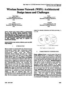
1.1 Literature Review On varying the transmission power of the nodes, it's number of neighbours can be varied. Assuming the disk graph model, we study the effect of varying the transmission power, and hence he transmission range on the size of the maximum connected component in randomly deployed wireless sensor network. A at network topology is assumed. On simulating a randomly deployed sensor network, with 5000 nodes in a 1500 x 1500 unit are with maximum transmission range of 100 units, the following plot was obtained:
Fig 1: Effect of power control on connectivity: number of connected nodes vs transmission range
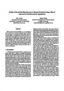
Clearly, in the case of dense deployment, 100 % connectivity can be obtained at relatively small transmission range. Therefore, by reducing the transmission range (by power control) can effectively achieve full connective. Also the size of the maxi-mum connected component does not gradually increase with transmission range, but increases sharply from 0 to maximum no. of components. Thus a phase transition and existence of a threshold can be seen. Relative Neighbourhood Graph (RNG) Andreas and willing presented a distributed approach to topology control in their book "Protocols and Architectures for Wireless Sensor Networks Protocols and Architectures for Wireless Sensor Networks". Sparsing a topology can be efficiently done locally if information about distance between nodes or their relative position is available, first we study the Relative Neighbourhood Graph. The Relative neighbourhood graph T of a graph G = (V, E) is defined as T = (V, E') where there is an edge between nodes u and v if and only if there is no other node w ( a witness) that is closer to either u or v than u and v are apart from each other formally,
K. Hari Krishna et al. / Procedia Computer Science 79 (2016) 893 – 902
Fig 2: Relative Neighbourhood Graph
Fig 3: Gabriel Graph
where d (u, v) is the Euclidean distance .between two nodes. But a this algorithm does not guarantee a strong connectivity. Gabriel Graph(GG) Another algorithm presented by andreas and willing was the gabriel graph for sparsing the topology. The Gabriel Graph (GG) is defined similarly to the RNG; the formal definition for it's edges is The nodes were randomly deployed in a 250 x 250 unit square area. Each node having a transmission power of 100 units. Both RNG as well as GG sparse the topology. In case of RNG, for some nodes which are only a few hops apart in the original graph becomes very distant. Even though this algorithm has a stronger connectivity than RNG, its quantitative value cannot be determined. CLTC CLTC stands for Cluster Based Topology Control. It was proposed by Shen et. al. It is a hybrid topology control framework that achieves both scalability and strong connectivity. The framework proposes dividing the Topology configuration into three phases: • Cluster Formation: In the first phase clusters are formed from the nodes using a suitable clustering algorithm • Intra Cluster Topology Control: In the second phase a centralized topology control algorithm is used to de ne the topology of each cluster as a sub-network. • Inter Cluster Topology Control: In the third phase the clusters are connected to each other to form the final topology of the network. We present one implementation of this framework: CLTC-A which analyzes the message complexity of the network. The energy of the network was not dealt with in this paper. Saving energy is a very critical issue in wireless sensor networks (WSNs) since sensor nodes are typically powered by batteries with a limited capacity. Since the radio transmission is the main cause of power consumption in a sensor node, transmission/reception of data should be limited as much as possible. In wireless sensor networks, energy is considered a scarce resource: • The sensor nodes are battery operated. Nodes and hence the wireless sensor network has a limited lifetime. If transmission power is controlled, the network lifetime can be optimized 1.2 Options for Topology Control To compute a modified graph I out of a graph G representing the original network G, a topology control algorithm has a few options: The set of active nodes can be reduced (Vt € V ), for example, by periodically switching o nodes with low energy reserves and activation other nodes instead, exploiting redundant deployment in doing so. The set of active links/the set of neighbours for a node can be controlled. Instead of using all links in a network, some links can be disregarded and communication is restricted to crucial links. When a at network topology is desired (all nodes are considered equal), the set of neighbours of a node can be reduced by simply not communicating with some neighbours. There are several possible approaches to choose neighbours, but one that is obviously promising for a WSN is to limit the reach of a node's transmission typically by power control, but also by using adaptive modulation (using faster modulation is only possible over shorter distance) and using the improved
895
896
K. Hari Krishna et al. / Procedia Computer Science 79 (2016) 893 – 902
energy efficiency when communicating only with nearby neighbours.
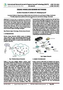
Fig 4: taxonomy of topology control problem
Active links/neighbours can also be rearranged in a hierarchical network topology where some nodes assume special roles. One example is to select some nodes as a "back-bone" (or a "spine") for the network and to only use the links within this backbone and direct links from other nodes to backbone.[5] 1.3 Taxonomy of Topology Control Problem The topology control problem can be broadly divided into two types based on the type of nodes deployed [6]: • homogeneous approach and heterogeneous approach IMPLEMENTING CLTC USING K-MEANS CLTC stands for Cluster Based Topology Control. It was proposed by Shen et. al. It is a hybrid topology control framework that achieves both scalability and strong connectivity. By varying the algorithms utilized in each of the three phases of the framework, a variety of optimization objectives and topological properties can be achieved. In this thesis, we present the implementation of CLTC framework for minimization of transmission power using kmeans clustering. The framework divides the TC problem into 3-phases: • Cluster formation • Intra Cluster topology Control • Inter Cluster topology Control We divide the construction of the network topology into the three aforementioned phases. In The first Phase, we use k-means for forming k distinct clusters out of the total N nodes in the network. Moreover, a cluster head is selected for each cluster. We assume in this phase that all nodes are transmitting at their maximum power and only connections possible are those within the cluster. Once clusters have been formed, each cluster modifies its topology using the relative neighborhood graph to further optimize the transmission power. These new trans-mission powers are stored with the nodes. The nodes do not start transmitting data at this point of time
Fig 5: A network without any Topology Control implementation
In the third phase, all pairs of clusters ui, uj try to connect to each other if the maxi-mum transmission range of the boundary nodes of ui can contact any boundary node of uj . For all such successful connections, the transmission
K. Hari Krishna et al. / Procedia Computer Science 79 (2016) 893 – 902
897
power of boundary nodes are set to the maximum of its present transmission power and the new value required to communicate with other clusters. 1.6
PHASE I: CLUSTER FORMATION
In the first phase, in a distributed fashion, clusters are formed and cluster heads are selected. Note that the operations in the subsequent two phases are independent of the specific clustering algorithm used in this phase. Any distributed clustering algorithm that can form non-overlapping clusters and select cluster heads can be applied. We use KMeans Clustering to form the clusters from the node deployed in the network as follows: At first we select K random nodes from the set of nodes N, these form the initial set of cluster heads then for each node ui, we find the closest cluster (using Euclidian Distance between nodes) head and label ui with the nodeID of this cluster head. Once all nodes have been assigned a label, we find the centroid of each cluster and label the node closest to the centroid as the new cluster head for the cluster. This process is repeated for R ( = N/10) number of times, to form the clusters. Algorithm 1 Clustering nodes for Phase I for i=1 to N/10 do clusterHeads[i] = rand()%M AX N ODES end for for i = 1 to 10 do for j = 1 to N do minDist = 1 for k = 1 to N/10 do newDist = distance(nodes[j]; nodes[clusterHeads[j]]) if newDist nodes[node2].power then nodes[node2].power = powerAssignment(minDist) end if end for end for 1.9
Simulation and Results
In this paper we present the Simulation of the network, the output plots and its analysis.
899
900
K. Hari Krishna et al. / Procedia Computer Science 79 (2016) 893 – 902
Simulation : For the Simulation of the Network, Omnet++ was used. OMNeT++ is an extensible, modular, component-based C++ simulation library and framework, primarily for building network simulators. First, we create a simple module called "node". This module contains all functionalities that the WSN nodes can carry out independently: • Sensing: data is generated virtually by each node, this data acts as the sensed data. • Computation: The computation done on data can be specified for each node. • Communication: The data is sent to other nodes by either specifying the out-put port to be used or the target node id. Then a network is created. We set the simulation area to 1000x1000 for this network and initialize the network with 100 nodes of the simple module created earlier. The topology of the network can be set in this network by specifying the connections between nodes. The network can now be simulated by running the project as a Omnet++ simulation. All simulation data and logs are saved to a file which can be used later for analysis.
Fig 8: Simulating a 100 node WSN ins Omnet++
1.10
Fig 9: Simulation results of 100 node WSN in Omnet++
Results
The results collected from the simulation were plot to a graph. We study the varia-tion average transmission power of nodes with the number of nodes in the network. We simulate the network in a constant area (of 1000x1000 unit area) with constant maximum transmission power of the nodes. 1.10.1 Average Transmission Power Vs. Number of Nodes The simulation if run 10 times for each value of number of nodes varying from 50 to 500 in intervals of 50 nodes and are averaged. The results obtained for networks with • No topology control • K-Means without CLTC • K-Means with CLTC are plot vs. the number of nodes.
Fig 10: plot of average transmission power. vs number of nodes
1.10.2 Node Power Depletion The simulation is run for 100 nodes and the node power depletion is plot for networks with no topology control, networks with k-means clustering and networks with CLTC implementation of k-means. 1.10.3 Node Lifetime The simulation is run for 100 nodes and the node lifetime is plot for networks with no topology control, networks with k-means clustering and networks with CLTC im-plementation of k-means.
K. Hari Krishna et al. / Procedia Computer Science 79 (2016) 893 – 902
901
1.11 Analysis From the Simulation and the Results Obtained we conclude that: • When no topology control is deployed and all nodes transmit at maximum power, the average transmission power of nodes is a constant (with the value =
Fig 11: node power depletion vs. time for network with no topology control Fig 12: node power depletion vs. time for network with no k-means cluster based topology control
Fig 13: node power depletion vs. time for network with CLTC:k-means based topology control Fig 14: node life time of 100 nodes for network with no topology control
Fig 16: node life time of 100 nodes for network with k-means cluster based topology control Fig 17: node life time of 100 nodes for network with CLTC:k-means based topol-ogy control maximum transmission power of the node)
• Simple K-Means shows a much lower average transmission power as compared to networks with no topology control. Moreover, the average transmission power in case of k-means decreases as the number of nodes in the network increases. • When CLTC is used, the average transmission power of the nodes is lesser than that of k-means, showing improvement. The transmission powers of nodes decreases with the increasing number on node deployment.
902
K. Hari Krishna et al. / Procedia Computer Science 79 (2016) 893 – 902
2.
Conclusion
We proposes modification to the CLTC framework so that it can be applied to Wireless Sensor Networks when the network lifetime has to be optimized. In order to do so, first of all we use a distributed approach in the second phase as compared to the centralized approach initially presented. This assures that the power consumption of cluster heads is minimized. The second is the implementation of the framework to minimize the node power consumption of nodes using k-means clustering, which is a simple clustering method to deploy in WSNs. We also present the effects of this implementation on node lifetime. Deployment of CLTC to Heterogeneous Networks: Our proposed work assumes a homogeneous network, but CLTC can be deployed to heterogeneous models as well. References 1. 2. 3. 4.
Hsiao Hwa Chen Konstantinidis Andreas, Yang Kun and Zhang Qingfu. Energy-aware topology control for wireless sensor networks using manetic algorithms. Mehdi Kalantari and Mark Shayman. Energy e cient routing in wireless sensor networks. In
Proc. of Conference on Information Sciences and Systems. Citeseer, 2004. Holger Karl and Andreas Willig. Protocols and Architechtures for Wireless Sensor Networks. John Wiley and Sons Inc., Norwell, MA, USA, 2005. 5. D. Minoli K. Shoraby and T. Znati. Wireless Sensor Network technology, protocols and applica-tions. Wiley-Interscience, Secaucus, NJ, USA, 2007. 6. M.R.Ebenezor Jebarani and T. Jayanty. An analysis of various parameters in wireless sensor networks using adaptive fec technique. International Journal of Ad hoc, Sensor Ubiquitous Computing, 1(3), 2010. 7. Paolo Santi. Topology control in wireless ad hoc and sensor netowrks. ACM computing Surveys, 37(3):164{194, 2005. 8. Rui Liu Zhuochuan Huang Jaikaeo Chaiporn Chien-Chung Shen, Chavalit Srisathapornphat and Errol L. Lloyd. Cltc: A cluster based topology control framework for ad hoc networks. IEEE transactions on mobile computing, 3(1), 2004. 9. Kheireddine Mekkaoui and Abdellatif Rahmoun. Short-hops vs. long-hops - energy eciency 10. analysis in wireless sensor networks. CEUR-WS, 825.