Networked Predictive Control for Time-varying ...

CEAI, Vol.13, No. 4, pp. 19-25, 2011

Printed in Romania

Networked Predictive Control for Time-varying Delay Compensation with an Application to Automotive Mechatronic Systems Constantin F. Caruntu, Corneliu Lazar Department of Automatic Control and Applied Informatics, ”Gheorghe Asachi” Technical University of Iasi, Str. Prof. dr. doc. Dimitrie Mangeron, nr. 27, 700050, Iasi, Romania (e-mail: {caruntuc,clazar}@tuiasi.ro). Abstract: The variable-time delay introduced by communication networks is the main factor that deteriorates the performance of Networked Control Systems (NCSs). In this paper, a new networked predictive control strategy is proposed with the aim of controlling the output of a physical plant, while compensating the effects of the time-varying delay. It is assumed that the delays in the communication network are bounded and three methods of considering the delays by the predictive control algorithm are proposed. Furthermore, a new method by which the controller is adapted to the difference between the desired reference and the plant output is proposed. Then, the proposed strategy is applied in order to control the clutch piston displacement and to decrease the influence of the variable-time delay induced in the NCS on the control performance of an electro-hydraulic actuated wet clutch. The performance of the proposed strategy is demonstrated by simulation results and corresponding comparisons prove the significance of this method. Keywords: Predictive Control, Networked Control Systems, Time-Varying Delay, Delay Compensation, Wet Clutch Control. 1. INTRODUCTION Feedback control systems over real-time communication networks, also called Networked Control Systems (NCSs), are now widely used in different industries, ranging from automated manufacturing plants to automotive and aero-spatial applications. These NCSs have many attractive advantages which include low cost, simple installation and maintenance, increased system agility, higher reliability and greater flexibility (Jiangang et al., 2007), but the use of communication networks makes it necessary to deal with the effects of the networkinduced delays in the control loop. These delays may be unknown and time-varying and may deteriorate the performances of the control systems designed without considering them and even destabilize the closed-loop control system (Jiangang et al., 2007). Existing constant time-delay control methodologies may not be directly suitable for controlling a system over a communication network since network delays are usually unpredictable and time-varying. Therefore, to handle network delays in a closed-loop control system over a communication network, an advanced methodology is required, a significant emphasis being on developing control methodologies to handle the network delay effect in NCSs (Tipsuwan and Chow, 2003). Various research has been on compensating the time-varying delays induced in NCSs and numerous control strategies were reported in the literature: multiple-delay Smith predictor based controller for systems with bounded uncertain delay (Ibeas et al., 2007), variable-period sampling scheme for NCSs with random time delay based on back-propagation neural network prediction (Jiangang et al., 2007), Smith dynamic predictor combined with fuzzy immune PID control (Du and Qian, 2008),

predictive networked controller based on Smith predictor that includes an adaptation loop to decrease the influence of the communication delay on the control performance (Velagic, 2008) and even model predictive control (Gielen and Lazar, 2009). The predictive control strategies were initially utilized for slow processes: oil refineries, petrochemicals, pulp and paper, primary metal industries, gas plant (Tran and Vlacic, 2006), but starting with the evolution of hardware components and algorithms, the possibility to implement these types of control algorithms to fast processes, which have reduced sampling periods, appeared: vehicle engine and traction control, aero-spatial applications, autonomous vehicles, power generation and distribution (Gu et al., 2009). As such, in order to decrease the influence of the time-varying delay induced in a NCS on the control system performance, in this paper, a networked controller based on a new predictive strategy is proposed, the delays that appear in the NCS being taken into account by the presented strategy. It is assumed that the delays in the communication network are bounded and three methods of considering the delays by the predictive control algorithm are proposed: an average delay method, an identification method, which uses an estimated model that includes the delays in the plant model, and an adaptation method, which adapts the control algorithm to the time-varying delays in the communication network. Furthermore, a new method by which the controller is adapted to the difference between the desired reference and the plant output is proposed. The strategy is then tested on a network-controlled wet clutch actuated by an electro-hydraulic valve, which is a subsystem

20

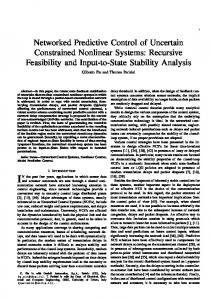
C ONTROL E NGINEERING AND A PPLIED I NFORMATICS The delays τ sc and τ ca are composed of at least the following parts (Tipsuwan and Chow, 2003): waiting time delay τ W , frame time delay τ F and propagation delay τ P . These three delay parts are fundamental delays that occur on a local area network, e.g., CAN.. When the control or sensory data travel across networks, there can be additional delays such as the queuing delay at a switch or a router and the propagation delay between network hops. The delays τ sc and τ ca also depend on other factors such as maximal bandwidths from protocol specifications and frame or packet sizes. In fact, both network delays can be longer or shorter than the sampling time Ts . Although the controller processing delay τ c always exists, this delay is usually small compared to the network delays and could be neglected. 3. NETWORKED PREDICTIVE CONTROL STRATEGY

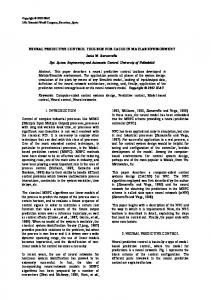
Fig. 1. NCS configuration and network delays. of the automatic transmission of a Volkswagen vehicle and the main control goal is to make the clutch plates position track a given external reference. Comparisons were made with two different networked controllers: a PI controller and a Smithlike predictive controller with adaptation to communication delay developed in (Velagic, 2008), in order to illustrate the performance of the proposed method. The effectiveness of the proposed solution is shown by a performance analysis on a set of simulation results. This paper is organized as follows. Section 2 describes the timevarying network-induced delays and in Section 3, the predictive control strategy is presented. Section 4 describes, firstly, the model of the valve-clutch system and, secondly, consists of the experimental results and discussion. The paper ends with a concluding chapter in Section 5. 2. DELAYS IN NCSS NCSs are composed of a central controller and a remote system containing a physical plant, sensors and actuators (Fig. 1). The controller and plant are located at different spatial locations and directly connected through a network to form a closed control loop (Yang et al., 2006). When sensors, actuators and controllers exchange data across the network, various delays with variable length occur due to sharing the common network medium. These delays are called network-induced delays and can vary widely according to the transmission time of messages and the overhead of the network. Usually, these network delays are randomly time-varying (Rodriguez and Menendez, 2007) and can be categorized from the direction of data transfers as the sensor-to-controller delay τ sc and the controller-to-actuator delay τ ca . Generally, both the controller and the actuator are event-driven and the sensor is time-driven, sampling the plant output every period. When one sampling begins, the data sampled by the sensor y (k) will be sent to the controller via the communication network, the delay τksc occurring during this interval. Then, the controller computes the control data u (k) according to the sampling data and then the control data will be sent to the actuator via the communication network, the delay τkca occurring in this interval. The actuator acts on the plant in no time once it receives the control data.

Predictive control techniques have been introduced mainly in order to deal with plants that have complex dynamics (unstable inverse systems, time-varying delay, etc.) and plant model mismatch. They are of a particular interest from the point of view of both broad applicability and implementation simplicity, being applied on large scale in industry processes, having good performances and being robust at the same time. Consider the plant described by the CARIMA (Controlled AutoRegressive Integrated Moving Average) model (Camacho and Bordons, 2004) e (k) C z −1 −1 −d −1 A z y (k) = z B z u (k − 1)+ , (1) D (z −1 ) where d is the delay of the process and e(k) is white noise with zero mean value. A z −1 and B z −1 are the system polynomials A z −1 = 1 + a1 z −1 + ... + anA z −nA , (2) B z −1 = b0 + b1 z −1 + ... + bnB z −nB , where nA and nB represent the polynomials degrees and C z −1 and D z −1 are the disturbances polynomials C z −1 = 1, (3) D z −1 = 1 − z −1 . 3.1 Prediction model The prediction model is given by yˆ (k + j|k) = Gj−d z −1 D z −1 z −d−1 u (k + j) + (4) Hj−d z −1 D z −1 Fj−d z −1 u (k − 1) + y (k) + C (z −1 ) C (z −1 ) with j = hi, hp, where hi is the minimum prediction horizon and hp is the prediction horizon. u(k + j − 1 |k ), j = 1, hc is the future control, computed at time k and yˆ (k + j|k) are the predicted values of the output, hc being the control horizon. For determining the polynomials Fj−d z −1 , Gj−d z −1 and Hj−d z −1 two Diophantine equations are used. The first is: C z −1 Fj−d z −1 −1 −(j−d) = Ej−d z +z , A (z −1 ) D (z −1 ) A (z −1 ) D (z −1 ) (5) where Ej−d z −1 = 1 + e1 z −1 + ... + enE z −nE , (6) Fj−d z −1 = f0 + f1 z −1 + ... + fnF z −nF ,

C ONTROL E NGINEERING AND A PPLIED I NFORMATICS

21

with nE = j − d − 1, nF = max (nA + nD − 1, nC − (j − d)) . The second Diophantine equation is Ej−d z −1 B z −1 = C z −1 Gj−d z −1 + +z −(j−d) Hj−d z −1 , where Gj−d z −1 = g0 + g1 z −1 + ... + gnG z −nG Hj−d z −1 = h0 + h1 z −1 + ... + hnH z −nH , with: nG = j − d − 1, nH = max (nC , nB + d) − 1.

(7)

−

−

(10)

T

J = (Gud + y ˆ0 − w) (Gud + y ˆ0 − w) + λud T ud , (18) subject to D(z −1 )u(k + i) = 0 for i ∈ [hc, hp − d − 1], where w is the reference trajectory vector with the components w(k + j |k ), j = hi, hp. Minimizing the objective function (∂J/∂ud = 0), the optimal control sequence yields as −1 T u∗d = GT G + λIhc G [w − y ˆ0 ] . (19) Using the receding horizon principle and considering that γj , j = hi, hp are the elements of the first row of the matrix −1 T GT G + λIhc G , the following control algorithm results: u (k) =

j=hi

hp X

γj Fj−d (z −1 )y(k) +

hp X

γj C(z −1 )w(k + j),

j=hi

3.2 Delay modeling

The objective function is based on the minimization of the tracking error and on the minimization of the controller output, the control weighting factor λ being introduced in order to make a trade-off between these objectives

D z

(21)

j=hi

y ˆ0 = [ˆ y0 (k + hi |k ), yˆ0 (k + hi + 1 |k ), . . . , yˆ0 (k + hp |k )]T . (17)

hp X

γj Hj−d (z −1 )D(z −1 )u(k − 1)−

(9)

Considering as inputs D(z −1 )u(k) and collecting the j-step predictors in a matrix notation, the prediction model can be written as y ˆ = Gud + y ˆ0 (13) where y ˆ = [ˆ y (k + hi |k ), yˆ(k + hi + 1 |k ), . . . , yˆ(k + hp |k )]T , (14)   ghi−d−1 . . . g0 0 . . . 0  ghi−d . . . g1 g0 . . .  0   ... ... ... ... ... , G =  ... (15)  g  g0 hc−1 . . . . . . . . . . . . ghp−d−1 . . . . . . . . . . . . ghp−hc−1 T −1 ud = D(z )u(k), . . . , D(z −1 )u(k + hc − 1) , (16)

hp X j=hi

(8)

The prediction model yields as yˆ (k + j|k) = Gj−d z −1 D z −1 z −d−1 u (k + j) + (11) +ˆ y0 (k + j|k) where Hj−d z −1 D z −1 u (k − 1) + yˆ0 (k + j|k) = C (z −1 ) (12) Fj−d z −1 y (k) + C (z −1 ) represents the free response.

−1

With yˆ0 (k + j|k) from (12), the control algorithm can be rewritten as C(z −1 )D(z −1 )u(k) =

γj [w (k + j |k ) − yˆ0 (k + j |k )]. (20)

Consider that the delay introduced by the communication network dc is time-varying, but bounded dm ≤ dc ≤ dM , (22) where dm is the minimum delay and dM is the maximum delay that appear in the communication network. In this paper, three methods of considering the communication delay proposed to be used by the predictive algorithm (Caruntu and Lazar, 2009; Caruntu et al., 2010) are discussed, which will be presented in the sequel. Average method The delay considered by the prediction model is calculated using dm + dM . (23) d= 2 Identification method The delay is considered equal to the minimum delay that can appear in the communication network d = dm (24) ˜ and instead of the polynomial B, another polynomial B, identified in order to model the system including the delays between dm and dM is introduced ˜ z −1 = ˜b0 + ˜b1 z −1 + ... + ˜bn z −nB˜ , B (25) ˜ B with nB˜ = nB + dM − dm , ˜b0 = ˜b1 = ... = ˜bn = b0 + b1 + ... + bnB , (26) ˜ B nB˜ + 1 ˜ B(1) = B(1), Adaptation method lated using

At each sampling time the delay is calcuN P

d=2

τ sci

i=1

, (27) N where τ is the communication delay from sensor-to-controller in i-th step. In this way, the average value of N previous delays is calculated. sci

The adaptation method is designed in order to adapt the control algorithm to the variable-time delays that appear in the communication network. The adaptation algorithm is derived with assumption that the average communication delays from sensor-to-controller and from controller-to-actuator are equal, both being variables. Unlike for the other two modeling methods, in the case of the adaptation method the upper bound of the delays can be unknown.

22


3.3 λ-scheduling Being known that λ is the parameter used to make the tradeoff between the minimization of the tracking error and the minimization of the controller output, it is easy to observe that by increasing λ, the process output tracks the reference more slowly, and by decreasing λ, the process output tracks the reference faster, but with an overshoot, as it will be shown in Subsection 4.2. So, the proposed solution is to modify the parameter λ on-line depending on the error between the desired reference and the process output. Consider the following error ykr − yk , ykr which takes values in the interval [1, 0]. ek =

(28)

Then, λ can be calculated using - linear functions: λk = a1 ek + b1 , - nonlinear functions: λk = a1 e2k + b1 ek + c, - piecewise affine (PWA) functions:  a1 ek + b1 , ek ∈ [e1 , e2 ],    a2 ek + b2 , ek ∈ (e2 , e3 ], λk =  ··· ,   aN ek + bN , ek ∈ (eN , eN +1 ],

(29) (30)

(31)

where ai , bi and c are suitable chosen constants, for i = 1, N . Now, considering that λmin and λmax are two values sufficiently small and large, respectively, for λ, it is easy to make a connection between ek and λk such that λk = (1 − ek )(λmax − λmin ) + λmin = (32) = −(λmax − λmin )ek + λmax , so, as the error ek decreases, the parameter λk increases. 4. ILLUSTRATIVE EXAMPLE Clutch control is seen more and more as an important enabling technology for the automotive industry, being central for automatic gear shifting and traction control for improved safety, drivability, comfort and fuel economy. During the last years this topic has been actively researched and the attention has focused on modelling and developing control methods for automated clutch actuators (Morselli et al., 2003; Van Der Heijden et al., 2007; Langjord et al., 2008; Neelekantan, 2008). All of the above control solutions assume that the sensors, controllers and actuators are directly connected, which is not realistic. Rather, in modern vehicles, the control signals from the controllers and the measurements from the sensors are exchanged using a communication network, e.g., Controller Area Network (CAN) or Flexray, among control system components. This brings up a new challenge on how to deal with the effects of the network-induced delays and packet losses in the control loop. In this paper, a network-controlled wet clutch actuated by an electro-hydraulic valve is used to illustrate the effectiveness of the proposed delay modeling methodology and the performance of the proposed predictive control scheme. The goal of the

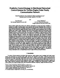
Fig. 2. Charging phase of the valve clutch system (dashed discharging phase). control algorithm is to achieve zero steady-state error and fast response of the valve-clutch system to step references for the clutch piston displacement, while compensating the timevarying delays introduced by CAN.

4.1 Valve-clutch system model The model of the valve-clutch system, which is represented in Fig. 2, designed based on physical principles for flow and fluid dynamics, is briefly described below by the following equations (Balau et al., 2009; Lazar et al., 2010): - force balance for the valve plunger: Fmag − AC PC + AD PD = Mv s2 x + Ke x

(33)

with Fmag =

ka i2 2(kb + x)

2,

LS

di + RS i = u, dt

(34)

where Fmag is the electromagnetic force that acts on the plunger, PC represents the oil pressure in chamber C exerted on area AC on the left end of the plunger, PD represents the oil pressure in chamber D exerted on area AD on the right end of the plunger, Mv is the plunger mass, Ke = 0.43w(PS0 − PR0 ) is the flow force spring gradient, Ps is the supply pressure, PR is the reduced pressure, w represents the area gradient of the main orifice, x represents the displacement of the plunger, s is the Laplace operator, ka and kb are constants, Ls the solenoid induction and Rs the resistance, i is the current in the solenoid and u is the input voltage; - flow continuity in the chambers C, D, R and L: QC = K1 (PR − PC ) =

VC sPC − AC sx, βe

(35)

QD = K2 (PR − PD ) =

VD sPD + AD sx, βe

(36)


23 4.2 Simulation results

−3

Clutch displacement [m]

x 10

PRBS valve−clutch system ARX

6

This section presents the validations of the proposed predictive control strategy investigated on the valve-clutch system model using the Matlab/Simulink program.

4 2 0 0

0.5

1 Time [s]

1.5

2

Fig. 3. Valve-clutch and simulation models responses. KC (PS − PR ) − QL − kl PR − K1 (PR − PC ) − Vt − K2 (PR − PD ) + Kq x = sPR , βe QL + K1 (PC − PR ) + K2 (PD − PR ) − Vt − KD (PR − PT ) − kl PR + Kq x = sPR , βe

(37)

VL sPL + AL sxp , (38) βe where K1 , K2 , K3 are the flow-pressure coefficients of the restrictors, KC is the flow-pressure coefficient corresponding to the main orifice, PL represents the oil pressure in the clutch chamber exerted on area AL , VC , VD , VL represent the chambers volumes, Kq is the flow gain of the main orifice, kl is the leakage coefficient, Vt represents the total volume of the chamber where the pressure is being controlled, βe is the bulk modulus and xp is the clutch displacement (output of the system); QL = K3 (PR − PL ) =

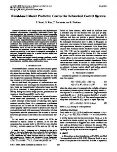
- force balance for the clutch piston: AL PL = Mp s2 xp + Kxp , (39) where K is the force flow spring rate for the clutch and Mp is the mass of the piston. Using the parameters estimated experimentally or already given by Continental Automotive Romania or the manufacturer (see Table A.1 in Appendix A), the model of the valve-clutch system was validated by comparing the simulation results with data obtained on a real test-bench at Continetal Automotive Romania (Lazar et al., 2010). In order to apply the predictive control strategy, a CARIMA model for the valve-clutch system was developed, using as input the supply voltage u and as output the clutch piston displacement xp . The system was identified with an ARX equivalent model employing the design model, utilizing as input a PRBS (PseudoRandom Binary Sequence) signal. These sequences are successions of squared pulses, width modulated, that approximate a discrete white noise and their richness in frequencies helps capturing the dynamical behavior of the system. The ARX model is given by the following system polynomials A z −1 = 1 − 1.781z −1 + 0.8039z −2 , (40) B z −1 = 0.00003312z −1 + 0.0001122z −2 . For disturbances model, the polynomial C is considered to equal one and D z −1 = 1 − z −1 for obtaining a zero steadystate error.

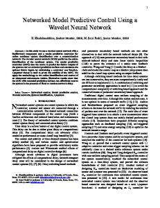
In this paper, the equation developed in (Herpel et al., 2009) it is used to determine the upper bound of the communication delays that appear on CAN in automotive applications (j + 2) · l , (41) dj ≤ Pj−1 R − i=0 (l/ci ) where l = 136 bits denotes the maximum frame length including the 6 bit CS time, R = 500 kbps is the rate of a high-speed CAN and ci is the cycle length of the i-th priority message and j is the priority of the node for which the upper bound is being calculated. A cycle length cn , corresponding to a message of priority n, represents the period after which the message is repeated. Using typical values for the parameters in (41), it yields that the sum of the delays (τ sc + τ ca ) is randomly distributed in the interval [0, 12Ts ], where Ts = 1ms is the sampling period of the system. Furthermore, being components of the same powertrain subsystem it can be considered that the communication delays from sensor to controller and from controller to actuator have the same values and they are uniformly distributed (see Fig. 4). The predictive control algorithm described in Section III was designed using the CARIMA model of the electro-hydraulic actuated clutch with the system polynomials from (40). It was considered that dm = 0 and dM = 12 from (41) and the predictive control strategy with the three methods was applied using the following parameters: hc = na + 1 = 3, hi = d + 1, hp = hc + d. The control action was then applied to the initial model of the valve-clutch system. The results obtained are compared with two different controllers: a PI controller and a Smith-like predictive controller with adaptation to communication delay developed in (Velagic, 2008). The λ-scheduling method was designed starting from the average delay method. As it can be seen in Fig. 5, for λ1 = 3 · 10−5 , the response of the system has a big overshoot, but it reaches the steady-state faster. For λ2 = 9.5 · 10−5 , the response of the system has no overshoot and it reaches the steady-state in a reasonable period of time, while for λ3 = 12 · 10−5 , the response of the system is really slow and for sure it has no overshoot. So, for λmin = λ1 and for λmax = λ3 , the relation (32) becomes: λk = −9 · 10−5 ek + 12 · 10−5 . (42) A step signal was applied as the reference for the clutch piston displacement and it was desired that the system tracks the reference signal as fast as possible, the following figures showing the controlled outputs and the reference signal. In Fig. 6 the clutch displacements obtained using the PI controllers and the Smith predictor are represented. Fig. 7 illustrates the reference clutch displacement value and the responses of the system with communication delay when the predictive strategy is applied. It can be seen that the system tracks the reference signal, having no steady state error and it has a rise time in accordance with the needs in this kind of automotive applications.

24

C ONTROL E NGINEERING AND A PPLIED I NFORMATICS −3

x 10

5

0.01


Communication delay [s]

0.012

0.008 0.006 0.004 0.002 0

0

0.05

0.1

0.15 Time [s]

0.2

0.25

4 3

1 0

0.3

reference average identification adaptation λ−scheduling

2

0

−3

0.2

0.25

0.3

1

x 10

Voltage [V]


0.15 Time [s]

0.8 4 λ1

2

λ2

0

0.05

0.1

0.15 Time [s]

0.2

0.25

0.6 0.4

0

0.3

Fig. 5. Clutch displacements for different λs. x 10

0.05

0.1

0.15 Time [s]

0.2

0.25

0.3

1 0.8 Voltage [V]

4 3 reference PI without delay PI with delay Smith predictor with delay

1 0

0.05

0.1

0.15 Time [s]

0.2

0.25

0.6 average identification adaptation λ−scheduling

0.4 0.2 0

0.3

Fig. 6. Clutch displacements. The responses are clearly different from those obtained with the PI controller and the Smith predictor. The set-point response for the PI and the Smith-like predictive controllers have an obvious overshoot, while the set-point curves for the predictive methods are similar except that the rise time for the adaptation and λscheduling methods is much smaller than those for the other methods and all the responses have almost no overshoot. In Fig. 8, the voltage signals (control signals) for the PI controllers and for the Smith predictor were represented. Fig. 9 illustrates the voltage signals (control signals) for the predictive methods. It can be seen that the variations of the voltage signal are much smaller for the proposed identification method, while the variations are much bigger for the adaptation method. Also, in Fig. 10, the delay used by the average method is represented and compared with the value of the delay used by the adaptation method for N = 20 from (27). It can be concluded that the performances of the predictive control methods are better than the performances of the Smith predictor proposed in (Velagic, 2008).

0

0.05

0.1

0.15 Time [s]

0.2

0.25

0.3

Fig. 9. Voltage signals. Average communication delay [Sampling periods]

2

0

0

Fig. 8. Voltage signals.

−3

5

PI without delay PI with delay Smith predictor with delay

0.2

λ3 0


0.1

Fig. 7. Clutch displacements.

Fig. 4. Time distribution of communication delay. 6

0.05

8 6 4 2 0

average adaptation 0

0.05

0.1

0.15 Time [s]

0.2

0.25

0.3

Fig. 10. Average communication delay. 5. CONCLUSION In order to overcome the influences of communication delays on the NCS performance, a new networked predictive control strategy is proposed in this paper. The strategy was then applied to control a wet clutch actuated by an electro-hydraulic valve

C ONTROL E NGINEERING AND A PPLIED I NFORMATICS with the aim of decreasing the influence of the communication time-varying delays on the closed-loop control performances over CAN. Comparisons were made with a PI controller and a Smith-like predictive controller with adaptation to communication delay developed in (Velagic, 2008), in order to illustrate the performance of the proposed approaches. The experiments designed to test the strategies developed in this paper verify the better performances of the proposed methods. ACKNOWLEDGEMENTS The work was supported by the National Center for Programs Management from Romania under the research grant SICONA - 12100/2008. REFERENCES Balau, A.E., Caruntu, C.F., Patrascu, D.I., Lazar, C., Matcovschi, M.H., and Pastravanu, O. (2009). Modeling of a pressure reducing valve actuator for automotive applications. In 18th IEEE International Conference on Control Applications, Part of 2009 IEEE Multi-conference on Systems and Control. Saint Petersburg, Russia. Camacho, E.F. and Bordons, C. (2004). Model Predictive Control. Springer Verlag. Caruntu, C.F., Balau, A.E., and Lazar, C. (2010). Networked predictive control strategy for an electro-hydraulic actuated wet clutch. In 6th IFAC Symposium Advances in Automotive Control, 419–424. Munchen, Germany. Caruntu, C.F. and Lazar, C. (2009). Predictive control for timevarying delay in networked control systems. In 8th IFAC Workshop on Time Delay Systems. Sinaia, Romania. Du, F. and Qian, Q.Q. (2008). Fuzzy immune self-regulating PID control based on modified Smith Predictor for networked control systems. In IEEE International Conference on Networking, Sensing and Control. Sanya, China. Gielen, R.H. and Lazar, M. (2009). Stabilization of networked control systems via non-monotone control Lyapunov functions. In 48th IEEE Conference on Decision and Control, 7942–7948. Shanghai, China. Gu, R., Bhattacharyya, S.S., and Levine, W.S. (2009). Dataflow-based implementation of model predictive control. In 28th American Control Conference. St. Louis, USA. Herpel, T., Hielscher, K.S., Klehmet, U., and German, R. (2009). Stochastic and deterministic performance evaluation of automotive can communication. Computer Networks, 53, 1171–1185. Ibeas, A., Vilanova, R., and Balaguer, P. (2007). Multiple-delay Smith Predictor based control of LTI systems with bounded uncertain delay. In 22nd IEEE International Symposium on Intelligent Control. Singapore. Jiangang, L., Biyu, L., Ruifang, Z., and Meilan, L. (2007). The new variable-period sampling scheme for networked control systems with random delay based on BP neural network prediction. In 26th Chinese Control Conference. Zhangjiajie, China. Langjord, H., Johansen, T.A., and Hespanha, J.P. (2008). Switched control of an electropneumatic clutch actuator using on/off valves. In 27th American Control Conference. Seattle, USA. Lazar, C., Caruntu, C.F., and Balau, A.E. (2010). Modelling and predictive control of an electro-hydraulic actuated wet clutch for automatic transmission. In IEEE Symposium on Industrial Electronics. Bari, Italy.

25 Morselli, R., Zanasi, R., Cirsone, R., Sereni, R., Bedogni, R., and Sedoni, E. (2003). Dynamic modeling and control of electro-hydraulic wet clutches. In IEEE Conference on Intelligent Transportation Systems. Shanghai, China. Neelekantan, V.A. (2008). Model predictive control of a two stage actuation system using piezoelectric actuators for controllable industrial and automotive brakes and clutches. Journal of Intelligent Material Systems and Structures, 19, 845– 857. Rodriguez, R.V. and Menendez, R.M. (2007). Network-induced delay models for can-based networked control systems. In 7th IFAC Conference on Fieldbuses and Networks in Industrial and Embedded Systems. Tipsuwan, Y. and Chow, M.Y. (2003). Control methodologies in networked control systems. Control Engineering Practice, 11, 1099–1111. Tran, T. and Vlacic, L. (2006). Practical process control techniques training. In 7th IFAC Symposium on Advances in Control Education. Madrid, Spain. Van Der Heijden, A., Serrarens, F., Camlibel, M., and Nijmeijer, H. (2007). Hybrid optimal control of dry clutch engagement. International Journal of Control, 80, 1717–1728. Velagic, J. (2008). Design of Smith-like predictive controller with communication delay adaptation. In World Congress on Science, Engineering and Technology, 5th International Conference on Control and Automation. Paris, France. Yang, C., Zhu, S., Kong, W., and Lu, L. (2006). Application of generalized predictive control in networked control systems. Journal of Zhejiang University, 7, 225–233.

Appendix A. PARAMETER VALUES

Table A.1. Valve-clutch parameter values

KC

Symbol

Value

Unit

Ke K Mv βe = KD K1 K2 K3 Kq w PS PT kl VC VD Vt VL AC AD AL α Mp ka kb Ls Rs

1000 900 25e-3 1.6e+9 7.58e-11 5.50e-10 3.52e-9 1.26e-8 5.3418 3e-3 1e+6 0 2e-9 7.53e-8 1.04e-7 3.2e-4 2.51e-5 3.66e-5 2.94e-5 7.75e-4 2e-5 0.5 0.005 0.01 0.01 0.5

[N/m] [N/m] [kg] [N/m2 ] [(m3 /s)/(N/m2 )] [(m3 /s)/(N/m2 )] [(m3 /s)/(N/m2 )] [(m3 /s)/(N/m2 )] [(m3 /s)/(N/m2 )] [m] [N/m2 ] [N/m2 ] [(m3 /s)/(N/m2 )] [m3 ] [m3 ] [m3 ] [m3 ] [m2 ] [m2 ] [m2 ] [m] [kg] [Nm 2 /A2 ] [m] [H] [Ω]