recognition of an electro hydraulic servo system (EHSS) in the presence of flow ... power are divided into two important branches of hydraulic and pneumatic.
IOSR Journal of Electrical and Electronics Engineering (IOSR-JEEE) e-ISSN: 2278-1676,p-ISSN: 2320-3331, Volume 8, Issue 1 (Nov. - Dec. 2013), PP 111-119 www.iosrjournals.org
Neural – Adaptive Control Based on Feedback Linearization for Electro Hydraulic Servo System Zohreh Alzahra Sanai Dashti*1, Milad Gholami2 and M. Aliyari Shoorehdeli3 1
Department of Electrical Engineering, Qazvin Branch, Islamic Azad University Qazvin, Iran 2 ABA Institute of Higher Education, Abyek, Iran 3 Mechatronics Department, Electrical Engineering Faculty. K. N. Toosi University, Tehran
Abstract: Neural Adaptive based on feedback linearization is used in this study to control the velocity and recognition of an electro hydraulic servo system (EHSS) in the presence of flow nonlinearities as well as internal friction and noise. This controller consists of four parts: PID controller, feedback linearization controller, neural network controller and the neural network identifier. The feedback linearization controller is used to prevent the system state in a region where the neural network can be accurately trained to achieve optimal control. The combination of controllers produces a stable system which adapts to optimize performance. This technique, as shown, can be prosperously used to stabilize any selected operating point of the system with noise and without interference. All consequences achieved are validated by computer simulation of a nonlinear mathematical model of the system. The fore mentioned controllers have a vast range to control the system. We compare Neural Adaptive based on feedback linearization controller results with feedback linearization, back stepping and PID controller. Keywords: Electro Hydraulic servo system; feedback linearization; RBF; EHSS. I.
INTRODUCTION
An introduction to the hydraulic systems liquids is also uncompressible. This property has caused to use liquids as a proper means to exchange and transport work. Therefore, they can be used in designing which why simple can move extra resisting power with little motivating force, this property is called hydraulic. Nowadays, in very industrial process is, transporting power as a very cheap and highly accurate method is aimed at. In this regard, applying compressed liquid to transport and control power is a spreading in all industrial branches [1, 2]. Applications of liquid power are divided into two important branches of hydraulic and pneumatic. Pneumatic is used in cases where relatively low forces (about ton) and high speed movement is needed (such as the systems used in moving parts). Pneumatic is used in cases where relatively low forces (about ton) and high speed movement is needed (such as the systems used in moving parts of robots. While hydraulic system applications are basically in cases where high power and speedy accurate controls are desired [1, 2]. Because the EHSS has proper control over inertial and torque loads, it is widely used in industry. Furthermore it yields precise and immediate answers [1, 2]. EHSS can be classified according to the aimed function, velocity, torque, force etc. In the past, dozens of studies have been carried out regarding different ways of handling methods of electro hydraulic servo system (EHSS). Reference [3] gives more information in this regard. An intelligent CMAC, FNN neural controller that uses a feedback error learning approach appears in [4, 5] which is highly complicated and [3] explain ways based on feedback linearization and back stepping However, it is not easy , nor is it simple to design such controllers. Other control methods will appear in [6-13]. Here, we intend to analyze and propose an adaptation based on the feedback linearization controller as well as the identifier for the EHSS system. The rest of the paper is arranged as follows. Part II, contains the mathematical model of the EHSS system. Part III deals with the RBF controller, identifier, PID controller and adaptive controller in detail. Section IV discusses the simulation results of the proposed control strategies. In the end, the conclusion is given in Section V.
II.
COMPOSE A MATHEMATICAL MODEL OF THE SYSTEM
An outline of an electro hydraulic velocity servo system is shown in Fig. 1. The basic components of this system are: 1. Hydraulic power supply, 2. Accumulator, 3. Charge valve, 4. Pressure gauge device, 5. Filter, 6. Two-stage electro hydraulic servo valve, 7. Hydraulic motor, 8. Measurement device, 9. Personal computer, and 10. Voltage - to- current converter.
www.iosrjournals.org
111 | Page
Neural – Adaptive Control Based on Feedback Linearization for Electro Hydraulic Servo System
Fig. 1. Electro hydraulic velocity servo system
A mathematical representation of the system is derived using Newton’s Second Law for the rotational motion of the motor shaft. It is assumed that the motor shaft does not change its direction of rotation, x1>0.This is a practical assumption and in order to be satisfied, the servo valve displacement x3 does not have to move in both directions. This assumption restricts the entire problem to the region where x 3>0. If the state variables are as follows: 1. x1 is hydro motor angular velocity. 2. x2 is load pressure differential. 3. x3 is valve displacement. Then the model of the EHSS is given by:
x1
1 Bm x1 qm x2 qmc f ps jt
x2
2 Be vo
x3
1 Tr
1 ( ps x2 ) qm x1 cim x2 cd wx3
kr x3 kq
(1)
u
y x1 Where the nominal values of parameters are: j t = 0.03 kgm2- Total inertia of the motor and load referred to the motor shaft, qm = 7.96×10⁻⁷ m3/rad – volumetric displacement of the motor, Bm=1.1×10⁻³ Nms – viscous damping coefficient, Cf = 0.104 -dimensionless internal friction coefficient, VO = 1.2×10⁻⁴ m3 - average contained volume of each motor chamber, B e =1.391×10⁹ pa - effective bulk modulus, Cd=0.61 – discharge coefficient, Cim=1.69×10⁻¹¹ m3/pa.s - internal or cross-port leakage coefficient of the motor, P S=107 pa - supply pressure, ρ=850 kg/m3 - oil density, Tr=0.1 s - valve time constant, - kr=1.4×10⁻⁴ m3/s.v - valve gain, ka=1.66-4 m2/s - valve flow gain, w= 8π×10-3 m - surface gradient. The control objective is stabilization of any chosen operating point of the system. It is readily shown that equilibrium points of system are given by: X1N: Arbitrary constant value of our choice
X 2N X 3N
1 Bm x1N qmc f ps qm
(2)
qm x1N cim x2 N cd w
1
( ps x2 N )
With very simple linearization we can find out that the system is minimum phase which allows application of many different design tools. In [14] Alleyne and Liu developed a control strategy that guarantees global stability of nonlinear, minimum phase single-input single-output (SISO) systems in the strict feedback form by using a passivity approach and they later used this strategy to control the pressure of an EHSS.
www.iosrjournals.org
112 | Page
Neural – Adaptive Control Based on Feedback Linearization for Electro Hydraulic Servo System III.
NEURAL-ADAPTIVE CONTROLLER
The In this study it was tried to design a velocity controller for electrohydraulic servo system which is adaptive based on feedback linearization controller. This controller, as shown in figure 3, consists of four parts: linear feedback controller, a nonlinear feedback linearization controller, an adaptive neural network controller and a neural network identifier. The total control signal is computed as follows: (3) u(t ) u m(t )u (1 m(t ))u pid
Where
u pid
bk
ad
is the linear feedback control,
uad is the adaptive neural network control and ubk is the feedback
linearization control. The function m(t ) allows a smooth transition between the feedback linearization and adaptive neural network controllers, based on the location of the system state:
m(t ) 0 x(t ) Ad 0 m(t ) 1 otherwise m(t ) 1 x(t ) A C
(4)
Where the regions might be defined as in Fig.2.
Fig. 2. Membership functions
The feedback linearization controller is used to keep the system state in a region where the neural network can be accurately trained to achieve optimal control. The linear feedback controller is turned on (and the neural controllers is turned off) whenever the system drifts outside this region. The combination of controllers produces a stable system which adapts to optimize performance. It should be noted that this neural controller and neural identifier uses the radial basis neural network. The linear feedback control is PID controller and the feedback linearization control is input-output controller.
Fig. 3. block diagram of the Neural – Adaptive Controller
A. RBF neural network In this study, we use a type of neural networks which is called the radial basis function (RBF) networks. These networks have the advantage of being much simpler than the Perceptrons while keeping the major property of universal approximation of functions[15]. RBF networks are embedded in a two layer neural networks, where each hidden unit implements a radial activated function. The output units implemented a weighted sum of hidden unit outputs. www.iosrjournals.org
113 | Page
Neural – Adaptive Control Based on Feedback Linearization for Electro Hydraulic Servo System The input to a RBF network is nonlinear while the output is linear. Their excellent approximation capabilities have been studied in [16]. The output of the first layer for a RBF network is: 2 (5)
i ( x) exp(
x ci
2 i 2
), i 1, 2...., n.
The output of the linear layer is:
yi i 1 w ji i ( x) w j T , j 1, 2...., n. n
(6)
y R m are input vector and output vector of the network, respectively, and T [1 ,...., n ]T is the hidden output vector, n is the number of hidden neurons, w [w j1 ,...., w jn ] is
Where x R and n
the weights vector of the network, parameters
ci and i are centers and radii of the basic functions, ci i
respectively. The adjustable parameters of RBF networks are w, and . Since the network's output is linear in the weights, these weights can be established by least square methods. The adaptation of the RBF parameters
ci and i is a non-linear optimization problem that can be solved by gradient-descent method.
B. RBF Identifier for EHSS The output RBF1 neural network variable,
(u ) will be used as the signal-input for establishing a RBF2 neural
network model to calculate the identifier law,
z1 i 1 vi exp( n
u Mi 2i
2
z1 .The output of the identifier based on RBF2 networks is:
2
) vT Q, i 1, 2,..., n.
Where n is the number of hidden layer neurons, parameters functions and
(7)
M i and i are centers and radii of the basic
z1 is the final closed-loop identifier input signal.
z1 x1 x1d
(8)
E ( z1 z1 )2 Updated equation of the weighting parameters is:
E 2 v E 22 v
(9)
vnew vold 2 vnew vold
(10)
E z1 Q v v
(11)
Finally we can find updating rule as follow:
vnew vold 22 EQ
(12)
C. RBF controller for EHSS
(e)
The error variable, will be used as the single-input signal for establishing a RBF1 neural network model to calculate the control law, u. Then for the single-input and single-output case in this paper, the output of the controller based on RBF1 networks is:
www.iosrjournals.org
114 | Page
Neural – Adaptive Control Based on Feedback Linearization for Electro Hydraulic Servo System
u i 1 wi exp( n
e ci 2 i 2
2
) wT , i 1, 2,..., n
(13)
Where n is the number of hidden layer neurons and u is the final closed-loop control input signal. Updated equation of the weighting parameters is:
e2 w e wnew wold 21e w e z1 z1 u w w u w z1 z1 u u z1 z1 Q u Q u z1 uM 2v Q u 2 u w
(14)
wnew wold 1
(15)
(16) (17) (18) (19) (20)
Finally we can find updating rule as follow:
wnew wold 41 e Q
uM
(21)
2
D. PID controller for EHSS PID controllers are used in industrial control systems vast because they have a few parameters which need to be adjusted its parameters includes control signals which are proper with error between reference and real output (p), Integral and differential of error (I) and (D). t 1 d u (t ) k p e(t ) e( )d ( ) Td e(t ) Ti 0 dt
u (t )
Which and e(t ) are control signals and error. function equation 2 as follow:
(22)
k p Ti T , and d are parameters should be adjusted. Transfer
1 u ( s ) k p 1 Td s Ti s
(23)
The main characteristics of PID controllers are their capacity to remove stable state error in response to step input (because of Integration factor) and predict the output variance (if differential factor is used).
IV.
SIMULATION RESULTS
In this section, the results of simulation are shown. The parameters of the PID controller are chosen
k
4
such that p , i and d are 0.0317, 0.0405 and 4.05 10 respectively. The Neural Adaptive controller has been compared with feedback linearization controller, back stepping and PID controller. They are show in figures (4, 5, 6, and 7). Figures (4, 5, 6, and 7) show the system output, the
k
k
m(t )
signal controller and the system states without the presence of output noise. Figure 8 show the function . To show the capabilities of the controller introduced in this paper, Gaussian noises with follow property have been applied to the aimed system. www.iosrjournals.org
115 | Page
Neural – Adaptive Control Based on Feedback Linearization for Electro Hydraulic Servo System
0.01 N (0,1) : amp 0.01, vae 1, avr 0 0.1 N (0,1) : amp 0.1, vae 1, avr 0 1 N (0,1) : amp 1, va1 1, avr 0 Figures (9, 10, and 11) show the results of the experiment with the presence of output Gaussian noise. 250
200
x 1[rad/s]
150
100
50
Feedback Linearization[3] Back stepping[3] PID Neural Adaptive
0
-50
0
1000
2000
3000
4000
5000 6000 time[ms]
7000
8000
x Fig. 4. Simulation result 1 without output noise for
9000 10000
x1n 200rad / s
7
4
x 10
Feedback Linearization[3] Back stepping[3] PID Neural Adaptive
3.5 3
x 2[PA]
2.5 2 1.5 1 0.5 0
0
1000
2000
3000
4000
5000 6000 time[ms]
7000
8000
9000
10000
6 x2n 1.3 10 pa
x Fig. 5. Simulation result 2 without output noise for -4
8
x 10
Feedback Linearization[3] Back stepping[3] PID Neural Adaptive
7 6
x 3[m]
5 4 3 2 1 0 0
500
1000
1500
2000
2500 3000 time[ms]
3500
x Fig. 6. Simulation result 3 without output noise for
www.iosrjournals.org
4000
4500
5000
x3n 1.17 10
4
m
116 | Page
Neural – Adaptive Control Based on Feedback Linearization for Electro Hydraulic Servo System 5
U[V]
0
-5
-10
Feedback Linearization[3] Back stepping[3] PID Neural Adaptive 0
500
1000
1500 time[ms]
2000
2500
3000
Fig. 7. Simulation result u[v]
1 0.9 0.8 0.7
m(t)
0.6 0.5 0.4 0.3 0.2 0.1 0
0
1
2
3
4
5 time[s]
6
7
8
9
10
Fig. 8. Simulation result m(t)
8
200
6
x 2[Pa]
x 1[rad/s]
8
300
100 0 -100
x 10
4 2
0
5 time[s]
0
10
0
5 time[s]
10
-3
1.5
x 10
10
u [v]
x 3[m]
1
5
0.5
0
0
5 time[s]
0
10
0
1
2 3 time[s]
4
5
x1n 200rad / s, 0.01 N (0,1)
x Fig. 9. Simulation result 1 with output noise for
8
8
100
0
x 10
6
200
x 2[Pa]
x 1[rad/s]
300
4 2
0
5 time[s]
0
10
0
5 time[s]
10
-3
1.5
x 10
10
u [v]
x 3[m]
1
5
0.5
0
0
5 time[s]
10
0
0
x Fig. 10. Simulation result 1 with output noise for
1
2 3 time[s]
4
5
x1n 200rad / s, 0.1 N (0,1)
www.iosrjournals.org
117 | Page
Neural – Adaptive Control Based on Feedback Linearization for Electro Hydraulic Servo System 8
300
10
x 2[Pa]
x 1[rad/s]
200 100 0 -100
0
5 time[s]
5
0
-5
10
x 10
0
5 time[s]
10
-3
1.5
x 10
10
u [v]
x 3[m]
1
5
0.5
0
0
5 time[s]
10
0
0
1
2 3 time[s]
4
5
x1n 200rad / s,1 N (0,1) Results show that Neural Adaptive controller delivers the Hydro motor angular velocity to the desired velocity much more quickly than feedback linearization, back stepping and PID controllers and has shorter settling time than other controllers also show that in presence output noise Neural Adaptive controller is robust controller. In table I we compare Neural Adaptive based on feedback linearization controller result with other controllers.
x Fig. 11. Simulation result 1 with output noise for
Table I. Comparison results controllers Number
Controller
Maximum signal control (volt)
Settling time (SEC)
1
Neural Adaptive based on feedback linearization [purpose]
1.4
0.5
2 3 4
PID[4] FEL[17] Neural Networks[5]
-10 2.5 5
3 2.5 6
5
Feedback Linearization[3]
1.5
7
6
Back Stepping[3]
1.4
7
7 8
PDC[17] Mamdani Fuzzy[4]
3.5 1.4
3 11
9
Neural Fuzzy[4]
30
4
Table I show that Neural Adaptive based on feedback linearization controller has shorter settling time than other controllers and it has less Maximum signal control competed with other controllers.
V.
CONCLUSIONS
This paper introduced Neural Adaptive based on feedback linearization method for control and identification of electrohydraulic servo system which has practical uses in many industrial systems. In this paper, a Neural Adaptive control method for EHSS is proposed, which consists of four parts: the linear feedback controller, the feedback linearization control, the neural network controller and the neural network identifier. It should be noted that the linear feedback controller is PID controller type and this neural controller and neural identifier used the radial basis function (RBF) network controller and the radial basis function (RBF) network identifier. The radial basis output is a linear function of the network weights, which allows faster training and simpler analysis than is possible with multilayer networks. Neural Adaptive controller is designed for stabilization of EHSS system to the desired point in the state space. Results obtained from the simulation show the superiority of the control system suggested in this paper. Neural Adaptive controller has shorter settling time than other controllers. It is also robust in presence of output noise applied to the aimed system.
[1] [2] [3] [4]
REFERENCES Z. Jianhui and C. Siqin, "Modeling and simulation for application of electromagnetic linear actuator direct drive electro-hydraulic servo system," in Power and Energy (PECon), 2012 IEEE International Conference on, 2012, pp. 430-434. P. N. Pham, K. Ito, and S. Ikeo, "The application of simple adaptive control for simulated water hydraulic servo motor system," in Industrial Technology (ICIT), 2013 IEEE International Conference on, 2013, pp. 204-209. M. Jovanovic, "Nonlinear control of an electrohydraulic velocity servosystem," in American Control Conference, 2002. Proceedings of the 2002, 2002, pp. 588-593 vol.1. S. A. Mohseni, M. Aliyari, and M. Teshnehlab, "EHSS Velocity Control by Fuzzy Neural Networks," in Fuzzy Information Processing Society, 2007. NAFIPS '07. Annual Meeting of the North American, 2007, pp. 13-18. www.iosrjournals.org
118 | Page
Neural – Adaptive Control Based on Feedback Linearization for Electro Hydraulic Servo System [5] [6]
[7] [8] [9] [10]
[11]
[12] [13] [14] [15] [16]
[17]
H. Azimian, R. Adlgostar, and M. Teshnehlab, "Velocity control of an electro hydraulic servomotor by neural networks," in Physics and Control, 2005. Proceedings. 2005 International Conference, 2005, pp. 677-682. M. A. Shoorehdeli, H. A. Shoorehdeli, M. Teshnehlab, and J. Yazdanpanah, "Velocity Control of an Electro Hydraulic Servosystem," in Networking, Sensing and Control, 2006. ICNSC '06. Proceedings of the 2006 IEEE International Conference on, 2006, pp. 985-988. F. Poloei, M. Zekri, and M. Aliyari Shoorehdeli, "Fuzzy-LQR hybrid control of an electro hydraulic velocity servo system," in Hybrid Intelligent Systems (HIS), 2011 11th International Conference on, 2011, pp. 5-9. A. C. Aras, E. Kayacan, Y. Oniz, O. Kaynak, and R. Abiyev, "An adaptive neuro-fuzzy architecture for intelligent control of a servo system and its experimental evaluation," in Industrial Electronics (ISIE), 2010 IEEE International Symposium on, 2010, pp. 68-73. J. Tai and X. Zhao, "Simulation study on the electrohydraulic servo system based on the fuzzy control algorithm," in Informatics in Control, Automation and Robotics (CAR), 2010 2nd International Asia Conference on, 2010, pp. 218-221. L. Manlin, L. Guanghua, C. Shuangqiao, and F. Yongling, "ADR algorithm applied in electro-hydraulic servo system," in Electronic and Mechanical Engineering and Information Technology (EMEIT), 2011 International Conference on, 2011, pp. 18881891. H.-y. Yu and L.-p. Shi, "The study of tracking control of electro-hydraulic servo system with feed forward and fuzzy-integrate control," in Electronic and Mechanical Engineering and Information Technology (EMEIT), 2011 International Conference on, 2011, pp. 4409-4412. I. C. Yeh, Z. Xin-Ying, W. Chong, and H. Kuan-Chieh, "Radial basis function networks with adjustable kernel shape parameters," in Machine Learning and Cybernetics (ICMLC), 2010 International Conference on, 2010, pp. 1482-1485. Z. A. S. Dashti, M. A. Shoorehdeli, M. Gholami, and M. Teshnehlab, "Neural Adaptive control for electro hydraulic servo system," in Control Conference (ASCC), 2013 9th Asian, 2013, pp. 1-6. A. G. Alleyne and L. Rui, "Systematic control of a class of nonlinear systems with application to electrohydraulic cylinder pressure control," Control Systems Technology, IEEE Transactions on, vol. 8, pp. 623-634, 2000. N. Jifu, "Conditions for radial basis function neural networks to universal approximation and numerical experiments," in Control and Decision Conference (CCDC), 2013 25th Chinese, 2013, pp. 2193-2197. S.-F. Su, J.-T. Jeng, Y.-S. Liu, C.-C. Chuang, and I. J. Rudas, "Robust radial basis function networks based on least trimmed squares-support vector regression," in IFSA World Congress and NAFIPS Annual Meeting (IFSA/NAFIPS), 2013 Joint, 2013, pp. 1-6. A. Zare and M. Aliyari, "Design Fuzzy Controller For Electro Hydraulic Servo System By Using LMI " presented at the 13th student college of Iranian confrences 2011.
www.iosrjournals.org
119 | Page