Saturated Neural Adaptive Robust Output Feedback Control of Robot

AUT Journal of Modeling and Simulation AUT J. Model. Simul., 49(2)(2017)199-208 DOI: 10.22060/miscj.2017.12177.5010

Saturated Neural Adaptive Robust Output Feedback Control of Robot Manipulators: An Experimental Comparative Study M. Pourrahim, K. Shojaei*, A. Chatraei, O. Shahnazari Dept. of Electrical Engineering, Najafabad Branch, Islamic Azad University, Najafabad, Iran ABSTRACT: In this study, an observer-based tracking controller is proposed and evaluated experimentally to solve the trajectory tracking problem of robotic manipulators with the torque saturation in the presence of model uncertainties and external disturbances. In comparison with the state-of-the-art observer-based controllers in the literature, this paper introduces a saturated observer-based controller based on a radial basis function neural network. This technique helps the controller produce feasible control signals for the robot actuators. As a result, it efficiently diminishes the actuators saturation risk and consequently, a better transient performance is obtained. The stability analyses of the dynamics of the tracking errors and state estimation errors are given with the help of a Lyapunov-based stability analysis method. The theoretical analyses will systematically prove that the errors are semi-globally uniformly ultimately bounded and they converge to a small set around the origin whose size is adjustable by a suitable tuning of parameters. At last, some real experiments are performed on a laboratory robotic arm to illustrate the efficiency of the proposed control system for real industrial applications.

1- Introduction Many research efforts have been accomplished in the recent decades where the various nonlinear control methods have been utilized to address the controller design of robot manipulators with limited inputs. One interesting aspect is the design and development of output feedback controllers (OFBCs), that eliminate velocity sensors to improve the noise immunity and save the volume, cost, and weight of the robot control system [1-4]. A main deficiency in the most of available works in the literature is that they suppose robot actuators are able to receive every arbitrary amount of generated control signals. In reality, robot actuators are subjected to physical constraints which restrict the amplitude of the available torques. Some problems that may be the result of the implementation of controllers based on the unlimited available torque assumption are: (i) degraded link position tracking, and (ii) thermal and mechanical damage. To overcome this problem, some researchers have proposed saturated tracking controllers [5-11]. A controller with limited amplitude signals has been designed in [5] for robot manipulators in the presence of uncertainties in the dynamic and kinematic models. In [6], an adaptive controller with bounded signals and a guaranteed robustness performance has been proposed for the tracking control of robotic arms. Dixon et al. [7] have introduced a tracking control law for robotic arms with bounded torque inputs. Reference [8] has proposed a bounded feedback controller to solve the robot trajectory tracking problem with the saturation constraint. The saturation function such as the hyperbolic tangent one has been used to design bounded tracking controllers for robotic arms in [9-11] in which a PID controller has been The corresponding author; Email: [email protected]

Review History: Received: 18 November 2016 Revised: 11 February 2017 Accepted: 27 February 2017 Available Online: 12 March 2017 Keywords: Actuator saturation Adaptive robust control Observer-based control RBF neural networks Robot manipulators

employed in their schemes. Loria et al. [12] presented a global output feedback regulator with bounded signals for the first time for robotic manipulators in 1997. However, they have not addressed the control problem under model uncertainties. Later, this work was improved by the theory of singularly perturbed systems [13]. In this paper, mathematical properties of the hyperbolic tangent function, generalized saturation functions, adaptive robust techniques, and artificial neural network (ANN)-based estimation capabilities are efficiently combined to address the above problems by proposing a saturated output feedback controller (SOFBC) for the robot trajectory tracking problem for the first time. The remaining parts of this paper are categorized in the following order. In section 2, preliminaries and basic mathematical theories are presented. A saturated output feedback tracking control system is introduced in section 3. The experimental results are provided in section 4 to demonstrate the superiority of the proposed controller. Eventually, section 5 concludes the paper. 2- Preliminaries In this section, we briefly review some background materials required in this paper. 2- 1- Robotic Arm Model The dynamic equation of a rigid n-link direct-drive robot is demonstrated by the following form:

M (q )q + C (q , q )q + Dq + G (q ) + t d = ta

(1)

where the signals q ( t ) , q ( t ) , q( t ) ∈ R n represent the link position, velocity and acceleration vectors, respectively; M(q)∈Rn×n shows the inertia matrix and C ( q , q ) ∈ R n ×n denotes a matrix of the centripetal and Coriolis terms. The

199

K. Shojaei et al., AUT J. Model. Simul., 49(2)(2017)199-208, DOI: 10.22060/miscj.2017.12177.5010

matrix D∈Rn×n is the diagonal positive-definite damping matrix. The vector G(q)∈Rn points out the gravity effects; td(t)∈Rn is a vector of external disturbances and static friction, and ta=[ta1,ta2,...,tan]T∈Rn demonstrates a vector of input torques with t ai ≤ t ai max , i = 1, 2,..., n . The model (1) satisfies the following properties: Property 1 [10], [14], [15]: The mass and inertia matrices satisfy the important property M(q) = MT(q) > 0 such that 2 2 lm x ≤ x T M ( q ) x ≤ lM x ∀x , q ∈ R n ,and 0si(z) is called a generalized saturation one with bound Mi, if it is non-decreasing, locally Lipschitz, and meets the following items: 1. x s i ( x ) > 0, ∀x ≠ 0 2. s i ( x ) ≤ M i , ∀x ∈ R Lemma 1. Let si:R—>R:z—>si(z) be a generalized saturation

∀x 1 , x 2 , q , y ∈ R n ;

function which is strictly increasing and continuously differentiable with the bound Mi. Let k1 and k2 be positive parameters and s i′ : x → ds i / d x . Then, the following always hold. 1. y [ s i ( x + y ) − s i ( x ) ] > 0, ∀y ≠ 0, ∀x ∈ R

C ( q , x 1 ) x 2 ≤ lc x 1 x 2 , ∀x 1 , x 2 , q ∈ R n ,

s i′ ( x ) = 0 2. xlim →∞

2.3) C ( q , x 1 )= x 2 C ( q , x 2 ) x 1 , ∀x 1 , x 2 , q ∈ R n ; 2.4)

restricting their performance adjustment role. Assumption 1. The links position signals are measurable in real-time. Assumption 2. The reference trajectory qd(t) is selected such that Sup q d ( t ) < B dp , Sup qd ( t ) < B dv and Sup qd ( t ) < B da

C (q,x1 + x 2= ) y C (q,x1 ) y +C (q,x 2 ) y ,

∀lc ≥ 0;

Property 3 [14]-[15]: The vector of gravity is bounded as

G ( q ) ≤ lG , ∀q ∈ R n , where lG is an unknown positive

scalar constant. Property 4 [14]: The matrix D satisfies D = DT > 0, ld x 2 ≤ x T Dx ≤ lD x 2 ∀ x ∈ R n and 0Rn be a smooth bounded desired trajectory that is created by a timing law. The control objective of this study is to develop a control law for a robotic arm to address the trajectory tracking problem under the following conditions: 1. The parameters of the robot manipulator’s model are completely unknown and the robot is subjected to external disturbances; 2. The velocity signals are not measurable for the feedback; 3. The controller shall guarantee that input constraints are not violated in the sense that t a ≤ nt aM where taM=max{tai,max}, i=1,2,...,n, ∀t≥0. Subsequently, the actuator saturation problem is mitigated such that a poor transient response is prevented. 4. The controller gains can be adjusted freely without

200

8. s i ( k 1x

′ k1 x , ∀x ∈ R; ) ≤ s iM

9. From (8), it is clear that

2 ′ k 1 x s i ( k 1x ) s i ( k 1x ) ≤ s iM ′ k 1xs i ( k 1x ) , ∀x ∈ R; = s iM

10. From (4), it turns out that s i2 ( x ) ≤ s ′iM2 x 2 , ∀x ∈ R

.

Proof. See the reference [8]. As it is conventional in the literature of the adaptive control [16], a projection operator is presented here to force the parameter estimates to remain within a bounded convex set yq:={q∈Rp:g(q)≤0}, where g(q) is a constraint function on q which should be defined by the user based on a prior knowledge of q [16]. The vector of parameters’ estimates, i.e. qˆ ∈ R p , is provided by the following adaptive rule:

K. Shojaei et al., AUT J. Model. Simul., 49(2)(2017)199-208, DOI: 10.22060/miscj.2017.12177.5010 3- Bounded Nn-based OFBC (2)

where z ∈ R p ,and y q and d(yq) demonstrate the interior and the boundary of yq, respectively; nqˆ := ∇g ( qˆ ) is the outward unit normal vector at qˆ ∈d (y q ) ,where G∈Rp×p shows the adaptive gain matrix, that is symmetric and qˆ ( 0 ) ∈y q . 0

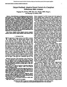
Lemma 2 [17]. A class of saturation functions shi(x) with the property |shi(x)|≤1,∀x∈R exist such that xshi(x)≥0 and h|x|≤xhshi(vhx/gd)+gd hold for any gd >0 and ∀x,h∈R where v denotes a parameter which satisfies the equality v=e−(v+1), that yields v=0.2785. 2- 4- RBF neural network In this subsection, RBFNN is presented to estimate uncertain nonlinear functions of the robot dynamics. Fig. 1 shows the structure of a three-layer RBFNN. This structure is extensively employed to approximate uncertain functions [14], [18].

3- 1- Controller development A bounded RBFNN-based adaptive robust OFB controller is designed here to meet the conditions (i)-(iv). To systematically design the observer and controller, the tracking error is specified by e(t):=q(t)−qd(t) and the state observation error is described by z(t):=q(t)−q̂(t). The signal q̂(t) shows the estimation of q(t). Then, the following signals are taken into account:

q= qd − Ls ( q − q d = ) qd − Ls ( e ) r r1 = q − qr = e + Ls ( e ) q = qˆ − Ls ( z )

(5) (6)

r2 = q − qo = z + Ls ( z )

(8)

(7)

o

where s(x):=[s1(x1),...,sn(xn)]T, ∀x∈Rn, s i (), i=1,...,n is defined by Definition 1, qr , qo ∈ R n are the variables of the controller and observer [19] and L= LT∈Rn×n shows a diagonal positivedefinite matrix. By inserting (6) in (1), and using Properties 2.3 and 2.4, the following open-loop error dynamics is achieved: −C ( q , q ) r1 − Dr1 + t a − C ( q , qr )e M ( q ) r1 = + M ( q ) Ls ′ ( e )e + C ( q , qd ) Ls ( e ) + D Ls ( e ) + x + xd − t d

(9)

where x =( M ( q d ) − M ( q ) ) qd + ( C ( q d , qd ) − C ( q , qd ) ) qd + ( D ( q d ) − D ( q ) ) qd + G ( q d ) − G ( q ) which is bounded as x ≤ B x s ( e ) 5, where B x = z M B da + z c B Fig. 1. A radial basis function neural network

An RBFNN for an arbitrary continuous function f(x):U—>Rp, where U denotes a compact set, is written in the following form: 

f (x ) = ∑w mk s k ( x ) + e m  x − mk  sk ( x ) = exp  − lk2   2

1, 2,… ,  k =

+ zG

by using Property .

Also, xd = −M ( q d ) qd − C ( q d , qd ) qd − Dqd − G ( q d ) is the desired computed dynamics of the robot, which is stated as = xd ( x d ) W s ( x d ) + e ( x d ) . Then, the following saturated neural network adaptive robust OFBC controller is proposed in this paper:

ta ( t ) = −s ( K 1qo − K 1qr ) −Wˆ s ( x d ) − αˆ s h ( v αˆ ( rˆ1 + rˆ2 ) / g d (t ) )

m = 1, 2,… , p ,

k =1

2 dv

(3)

(10)

where K = K 1T ∈ R n ×n is a matrix which is positive-definite. 1 The parameter αˆ and ANN weights matrix are generated by

where em is the approximation error of RBFNN, l and p are representing the number of nodes in the hidden and output  (11) layers, respectively, sk(x) is k-th Gaussian basis function Wˆ= ProjWˆ ( GW ( rˆ1 + rˆ2 )s T (x d ) ) where mk=[mk1, mk2,..., mkq]T shows the center vector and lk = αˆ Projαˆ (g α rˆ1 + rˆ2 ) denotes the standard deviation. Then, the nonlinear function (12) is stated by the following expression: where Gw and ga denote the adaptation gain matrices. It is (4) = f (x ) W s (x )+e necessary to mention that rˆ1 + rˆ2 is the approximation of r1+r2 which is given as follows: where f(x)=[f1(x),...,fp(x)]T, W∈Rp×l shows the matrix of weights, s(x)=[s1(x),...,sl(x)]T and e=[e1,e2,...,ep]T is bounded (13) rˆ1 + rˆ2 =: qˆ − qd + Ls ( e ) + Ls ( z ) as ||e||≤Be with the upper bound Be. Therefore, the uncertain nonlinear function is estimated as f̂(x)=Ŵs(x) where Ŵ The approximation rˆ1 + rˆ2 ≅ r1 + r2 can be confirmed if displays the estimation of the weights matrix, that should be the gains L and kd are selected large enough where kd is the updated by designing an adaptation rule.

201

K. Shojaei et al., AUT J. Model. Simul., 49(2)(2017)199-208, DOI: 10.22060/miscj.2017.12177.5010

gain of the state estimator, which will be introduced below. For the aim of the stability analysis in the next subsection, the approximation error is defined by

r1 + r2 =: r1 + r2 − ( rˆ1 + rˆ2 )= 2 ( r2 − Ls ( z ) )

from (6), (8) and (13) which is bounded as:

r1 + r2 ≤ x5 x

(6) and (8). The Properties 2.3 and 2.4 help write (22) as:

−C ( q , q ) r2 − k d M ( q ) r2 M ( q ) r2 = − s ( K 1r1 − K 1r2 ) − αˆ s h ( uαˆ ( rˆ1 + rˆ2 ) / g d (t ) ) +W s ( x d ) + e ( x d ) + c2 − td

(14)

where x5 represents a positive constant. Now, a velocity estimator is proposed as follows which is inspired by the reference [19]:

qˆ= ( t ) qˆo ( t ) + Ls ( z ( t ) ) + k d z ( t ) t qˆo ( t= ) qd ( t ) + k d L ∫ s ( z ( t ) ) d t

(15) (16)

0

where kd∈R shows the gain of the state estimator which is a positive constant. To run the observer, the initial values of the states are chosen as follows: qˆo ( 0 ) =− ( Ls ( z ( 0 ) ) + k d z ( 0 ) ) , qˆ ( 0 ) =q ( 0 ) = z ( 0 ) 0= and qˆ ( 0 ) 0

Then, considering that r1 − r2 = qo − qr from (6) and (8) and substituting (10) in (9), the closed-loop system error dynamics is achieved as follows: −C ( q , q ) r1 − Dr1 − s ( K 1r1 − K 1r2 ) M ( q ) r1 = −Wˆ s ( x d ) − αˆ s h ( v αˆ ( rˆ1 + rˆ2 ) / g d (t ) ) +W s ( x d ) + e ( x d ) + c1 − t d

where

(17)

(23)

where

c 2 =−Dr + D Ls ( e ) + C ( q , r1 + qr ) r2 − C ( q , r1 )( r1 + 2qr )

(24)

+ C ( q , Ls ( e ) ) ( qr + qd ) + x

From (3) and (4), Properties 2.5 and 4, and Lemma 1, an upper bound for c2 is acquired as follows:

c 2 ≤ x3 x + x 4 x

2

(25)

where x1 ,x2∈R are some positive parameters. 3- 2- Analysis of closed-loop stability The stability of the control system is analyzed here by the following theorem: Theorem 1: Let the dynamic model of robot manipulators be given by (1). Consider a continuous bounded desired trajectory under Assumptions 1–2. If the gains of the following proposed controller:

−s ( K 1qo − K 1qr ) −Wˆ s ( x d ) − u R ta ( t ) = = u R αˆ s h ( uαˆ ( rˆ1 + rˆ2 ) / g d (t ) )

 Wˆ= ProjWˆ ( GW ( rˆ1 + rˆ2 )s T (x d ) ) (18) + M ( q ) Ls ′ ( e )e + D Ls ( e ) + x = αˆ Projαˆ (g α rˆ1 + rˆ2 ) whose upper bound is expressed as follows by using rˆ1 + rˆ2 =: qˆ − qd + Ls ( e ) + Ls ( z )

c1 = −C ( q , qr )e + C ( q , qd ) Ls ( e )

Properties1, 2.5 and 4:

c1 ≤ x1 x + x 2 x

2

(19)

where x1,x2∈R are the positive upper-bounding constants. Also, x∈R4n is defined as follows:

x := [ s T ( e ) , s T ( z ) , r1T , r2T

]

T

(20)

 W −Wˆ If the weights matrix estimation error is defined by W= , one attains

W s ( x d ) + e ( x d ) −Wˆ s ( x d ) = W s ( x d ) + e ( x d )

lmin ( L ) > 0.5 ′ k 1M + 0.5 + 0.5 ( x1 + x 2 ) ld > s MM ′ k 1M + 0.5 + 0.5 ( x3 + x 4 ) ) lm k d > ( 2s MM

(26) (27) (28) n i =1,

(21)

By inserting (21) in (17), the following error dynamic equation is established:

M ( q ) r1 = −C ( q , q ) r1 − Dr1 − s ( K 1r1 − K 1r2 ) − αˆ s h ( uαˆ ( rˆ1 + rˆ2 ) / g d (t ) ) +W s ( x d ) + e ( x d ) − t d + c1

satisfy the following inequalities:

′ := max { s iM ′ } then, where k 1M = lmax ( K 1 ) and s MM the proposed bounded RBF neural network adaptive robust OFBC guarantees (i) the boundedness of all closed-loop signals, and (ii) the semi-global uniform ultimate boundedness (SGUUB) of the tracking and observation errors. In addition, an estimation of the region of attraction is given by  p R= ϑ ∈ ℜ ϑ < A 

2 b m − ( x1 + x3 + x5 )  ( x 2 + x 4 )( lϑ lx ) 

T where ϑ : [u = = ,w 11 ,...,w p  ,α ]T , u (22)

The time derivative of (15) results in qˆ= qˆo + Ls ′ ( z ) z + k d z

which is equal to r1= r2 + k d r2 + Ls ′ ( e ) e by applying

202

[ e T , z T , r1T , r2T ]

T

P=4n+pl+1, bm is a positive parameter which depends on control gains, xi, i=1,...,5 are defined in (14), (19) and (25), and lx and lu will be given later. Proof: See the appendix section

K. Shojaei et al., AUT J. Model. Simul., 49(2)(2017)199-208, DOI: 10.22060/miscj.2017.12177.5010 Remark 1 (guidelines for parameters tuning): In practical situations, the accurately tuning of the controller’s parameters is a little cumbersome and it is often done by the trial and error methods. In this remark, a few guidelines are given for the users to adjust the control parameters properly. The controller’s parameters K1, L, kd, Gw, ga and gd(t) should be tuned carefully to adjust the transient and steady-state performances. Based on Lyapunov stability analysis which is presented in the appendix section, the following laws are provided here for a trade-off between the robustness and the tracking performance of the control system: i. Controller and observer gains: The increasing of gains of the controller and the observer, i.e. K, L, and kd, increase the convergence rate cm in (41) and consequently lead to a smaller glim/cm. In addition, an arbitrary increase in K1 does not change the amplitude of the control signals in the present controller (10) by recalling the saturation function properties in Lemma 1. ii. Artificial neural network parameters: At first, a small number of neurons in the hidden layer are selected, then, one gradually increases this to gain a better performance for the trajectory tracking. The number of neurons is enough when there is no performance improvement. Large values of ANN gain, Gw, in (11) increase the rate of uncertain nonlinearities learning. However, it should be noted that the stability of the system might be jeopardized by choosing very large gains and the speed of learning is decreased by the selection of very small gains. iii. Adaptive robust control parameters: The increase of adaptive gain ga in the update rule (12) improves the robustness and the tracking performance of the controller. It should be noted that larger values of the adaptive gain ga may increase the roughness of the control signals. It in turn leads to an unwanted chattering in the control signals which is impractical for the robot motors due to their restricted bandwidth. One can make a trade-off between the smoothness of the controller signals and the final tracking accuracy by a finely tuning of the time function gd(t) in the controller (10). The controller (10) generates smoother signals by setting a large value of gd(t). However, it should be noted that a larger magnitude of gd(t) increases the magnitude of glim in (41). Hence, a larger ultimate bound, i.e. glim /cm, is resulted and, thus, the final tracking error will be increased.

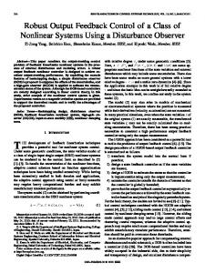
CPU microcontroller with 84 MHz clock frequency, 54 digital I/O pins (where twelve pins can be utilized for PWM outputs), 12 analog inputs and 4 UARTs (serial inputs of the hardware). The test bed consists of a 4-DOF SCARA industrial robot, decoder counter latch, MOSFET power amplifier and Arduino Due controller is connected to a computer as shown in Fig. 4. In this figure, the required hardware for the implementation of the proposed controller has been illustrated completely. The following saturation function is selected in this experiment to bound the tracking and estimation errors in order to evaluate the proposed saturated observer-based controller:   ηj + Lj   −L j + ( M j − L j ) tanh  M − L  , ∀η j < −L j j   j  s j (η j ) =  η j , ∀η j < −L j   L j + ( M j − L j ) tanh  η j − L j  , ∀η j < −L j  M −L   j   j

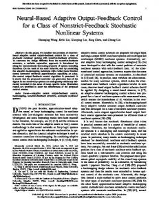
Fig. 2. SCARA IBM 7547 robot manipulator.

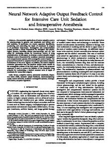
4- Experimental Evaluation 4- 1- Experimental results Here, the proposed controller is implemented on an industrial robot, SCARA IBM 7547 shown in Fig. 2. For the definition of the kinematics and dynamics of this type of robotic arms, the interested readers are referred to robotic textbooks [14-15] and references therein. This robot is a 4-DOF IBM 7547 SCARA robot manipulator which has three rotational joints and one prismatic joint is driven by gearbox DC motors equipped with incremental shaft encoders. The controller signals are converted to 40 KHz PWM signals with 13 bits resolution, which are directly applied to DC motors via IRF540N-MOSFET (H-Bridge technique) power amplifiers according to Fig. 3. The control system of the robot has been designed and implemented on an Arduino Due board. This board uses Atmel SAM3X8E ARM Cortex-M3

Fig. 3. MOSFET Power Amplifier

Fig. 4. The block diagram of the implementation system

203

(29

K. Shojaei et al., AUT J. Model. Simul., 49(2)(2017)199-208, DOI: 10.22060/miscj.2017.12177.5010

Fig. 5. Trajectory tracking results on SCARA IBM7547 robot manipulator without saturation: (a) robot and desired trajectories, (b) a magnified view of the trajectory, (c) controller output signals, and (d) the tracking errors.

Fig. 6. Trajectory tracking results on SCARA IBM7547 robot manipulator with : (a) robot and desired trajectories, (b) a magnified part of the trajectory, (c) controller output signals and (d) the tracking errors.

Fig. 7. Trajectory tracking results on SCARA IBM7547 robot manipulator with : (a) robot and desired trajectories, (b) a magnified view of the trajectory, (c) controller output signals and (d) the tracking errors. Table I. Quantitative comparisons

Performance index rms(e(t)) (m) rms(u(t)) (V) eM(m) ef(m)

Proposed controller in [2] Link 1 21.1701 14.9235 53.0414 1.1607

Proposed controller with tanh(.)

Link 2 10.1309 7.2507 21.4433 1.4758

Link 1 21.2460 13.0695 53.2399 0.8866

where Lj 0.5 ( x1 + x3 + x5 ) + 0.5 ( x 2 + x 4 ) x

compact set

2

(40)

2

+ g lim

Sx =

{ x (t ) 0 ≤

x (t ) ≤ g lim c m }

, which shows

E(t) is decreasing out of the set Sx. This gives the following result: 2 (42) E ( t ) ≤ E (0) ≤ lϑ ϑ (0) , ∀t ≥ 0

x

2

≤ lϑ / lx ϑ (0)

and

By considering (11) and (12) and Assumption 2, q can be bounded as ||q||≤qm. Then, by considering 2ab≤a2+b2 and recalling (14), one can re-write (36) as follows:

206

2

(43)

Thus, the following condition is sufficient to satisfy (40):

b m > 0.5 ( x1 + x3 + x5 ) + 0.5 ( x 2 + x 4 ) × ϑ

and considering (19) and (25) and recalling items (vii) and (viii) in Lemma 1, we obtain: 2 2 2 E ( t ) ≤ −lmin ( L ) s ( e ) − ld r1 − lmin ( L ) s ( z ) 2

− 0.5 ( x 2 + x 4 ) x

(l

T rˆ1 + rˆ2 αˆ − ( rˆ1 + rˆ2 ) αˆ s h ( uαˆ ( rˆ1 + rˆ2 ) / g d (t ) ) ≤ n g d ,

′ k 1M r2 + s MM

(38)

where we used inequality (32). By recalling (32) and (42), one has

+ α rˆ1 + rˆ2 − α Projαˆ (g α rˆ1 + rˆ2 ) / g α

2

are

(41) g : = lim g ( t ) where cm is also a positive scalar and lim t →∞ .This points out that E (t ) is strictly negative when x(t) is out of the

+ r ( s ( K 1r1 ) − s ( K 1r1 − K 1r2 ) )

− k d lm r2

+ g (t )

b1= b 2 = lmin ( L ) − 0.5 ′ k 1M + 0.5 + 0.5(x1 + x 2 ) ) b 3 = ld − ( s MM ′ k 1M + 0.5 + 0.5(x3 + x 4 ) ) b 4= k d lm − ( 2s MM

E ( t ) ≤ −c m x

− r1T s ( K 1r1 ) + r2T ( s ( K 1r1 ) − s ( K 1r1 − K 1r2 ) ) + r2

(37)

2

Then, inequality (39) can be written as

T 1

− r2T s ( K 1r1 ) + s ( e ) r1 + r1

2

where= g (t ) n g d (t ) + 0.5x5q m2 and bi , i = 1,, 4 defined as:

recalling

, and substituting (11), (12), inequality (34) is

E ≤ −lmin ( L ) s ( e )

− b 3 r1

E ( t ) ≤ −( b m − 0.5 ( x1 + x3 + x5 )

e − td ≤ α considering

4

2

The control parameters are set such that bi>0, i=1,...,4. As a result, the conditions of Theorem 1 are met. Thus, (37) may be expressed as follows:

A bound for the term e−td(t) is given as follows: By

− b2 s ( z )

+ 0.5 ( x1 + x3 + x5 ) x

+ 0.5 ( x 2 + x 4 ) x

= −s T ( e ) Ls ( e ) − r1T Dr1 − s T ( z ) Ls ( z )

T 2

2

2

/ lx ϑ (0)

2

)

(44)

The above equation hints that RA in Theorem 1 is an estimation of the attraction region whose size depends on the controller gains. As a consequence, ||x(t)|| is SGUUB. Therefore, this result helps us to find that e (t ), z (t ), r1 (t ), r2 (t ),Wˆ (t ), αˆ (t ) ∈ L ∞ by recalling the properties of saturation functions which are presented in Lemma 1. The above-mentioned argument is the evidence of SGUUB stability of the state estimation and tracking errors, weights, and parameters estimation errors. Furthermore, it is concluded that e(t ), z (t ) ∈ L ∞ by considering (6) and (8). At last, equations (6) and (8), the controller (10), and Assumption 2 show that

q (t ), qˆ (t ), q (t ), qˆ (t ), qr (t ), qo (t ), t a (t ) ∈ L ∞ . It is clear

that this statement completes the proof of Theorem 1. □

REFERENCES [1] H. Berghuis, H. Nijmeijer, A passivity approach to

K. Shojaei et al., AUT J. Model. Simul., 49(2)(2017)199-208, DOI: 10.22060/miscj.2017.12177.5010 controller-observer design for robots, IEEE Transactions on robotics and automation, 9(6) (1993) 740-754. [2] M.A. Arteaga, R. Kelly, Robot control without velocity measurements: New theory and experimental results, IEEE Transactions on Robotics and Automation, 20(2) (2004) 297-308. [3] D.J. López-Araujo, A. Zavala-Río, V. Santibáñez, F. Reyes, Output-feedback adaptive control for the global regulation of robot manipulators with bounded inputs, International Journal of Control, Automation and Systems, 11(1) (2013) 105-115. [4] M. Mendoza, A. Zavala-Río, V. Santibáñez, F. Reyes, Output-feedback proportional–integral–derivative-type control with simple tuning for the global regulation of robot manipulators with input constraints, IET Control Theory & Applications, 9(14) (2015) 2097-2106. [5] W.E. Dixon, Adaptive regulation of amplitude limited robot manipulators with uncertain kinematics and dynamics, IEEE Transactions on Automatic Control, 52(3) (2007) 488-493. [6] C. Huang, X. Peng, C. Jia, J. Huang, Guaranteed robustness/ performance adaptive control with limited torque for robot manipulators, Mechatronics, 18(10) (2008) 641-652. [7] W.E. Dixon, M.S. de Queiroz, F. Zhang, D.M. Dawson, Tracking control of robot manipulators with bounded torque inputs, Robotica, 17(2) (1999) 121-129. [8] E. Aguiñaga-Ruiz, A. Zavala-Río, V. Santibanez, F. Reyes, Global trajectory tracking through static feedback for robot manipulators with bounded inputs, IEEE Transactions on Control Systems Technology, 17(4) (2009) 934-944. [9] A. Laib, Adaptive output regulation of robot manipulators under actuator constraints, IEEE Transactions on Robotics and Automation, 16(1) (2000) 29-35. [10] Y. Su, P.C. Muller, C. Zheng, Global asymptotic saturated PID control for robot manipulators, IEEE Transactions on Control Systems Technology, 18(6) (2010) 1280-1288.

[11] V. Santibañez, K. Camarillo, J. Moreno-Valenzuela, R. Campa, A practical PID regulator with bounded torques for robot manipulators, International Journal of Control, Automation and Systems, 8(3) (2010) 544-555. [12] A. Loria, R. Kelly, R. Ortega, V. Santibanez, On global output feedback regulation of Euler-Lagrange systems with bounded inputs, IEEE Transactions on Automatic Control, 42(8) (1997) 1138-1143. [13] J. Moreno-Valenzuela, V. Santibáñez, R. Campa, On output feedback tracking control of robot manipulators with bounded torque input, International Journal of Control, Automation, and Systems, 6(1) (2008) 76-85. [14] F.L. Lewis, D.M. Dawson, C.T. Abdallah, Robot manipulator control: theory and practice, CRC Press, 2003. [15] M.W. Spong, S. Hutchinson, M. Vidyasagar, Robot modeling and control, Wiley New York, 2006. [16] P.A. Ioannou, J. Sun, Robust adaptive control, PTR Prentice-Hall Upper Saddle River, NJ, 1996. [17] B. Yao, Adaptive robust control of nonlinear systems with application to control of mechanical systems, University of California, Berkeley, 1996. [18] L. Xu, B. Yao, Output feedback adaptive robust precision motion control of linear motors, Automatica, 37(7) (2001) 1029-1039. [19] K. Shojaei, A. Chatraei, A Saturating Extension of an Output Feedback Controller for Internally Damped Euler‐Lagrange Systems, Asian Journal of Control, 17(6) (2015) 2175-2187. [20] M. Pourrahim, K. Shojaei, A. Chatraei, O.S. Nazari, Experimental evaluation of a saturated output feedback controller using RBF neural networks for SCARA robot IBM 7547, in: Electrical Engineering (ICEE), 2016 24th Iranian Conference on, IEEE, 2016, pp. 1347-1352.

Please cite this article using: M. Pourrahim, K. Shojaei, A. Chatraei, O. Shahnazari, Saturated Neural Adaptive Robust Output Feedback Control of Robot Manipulators: An Experimental Comparative Study, AUT J. Model. Simul., 49(2)(2017)199-208. DOI: 10.22060/miscj.2017.12177.5010

207

K. Shojaei et al., AUT J. Model. Simul., 49(2)(2017)199-208, DOI: 10.22060/miscj.2017.12177.5010

208