Hindawi Publishing Corporation Mathematical Problems in Engineering Volume 2016, Article ID 6153749, 14 pages http://dx.doi.org/10.1155/2016/6153749
Research Article Neural Architectures for Correlated Noise Removal in Image Processing Cstslina Cocianu and Alexandru Stan Computer Science Department, Bucharest University of Economics, 010552 Bucharest, Romania Correspondence should be addressed to C˘at˘alina Cocianu;
[email protected] Received 21 January 2016; Accepted 24 March 2016 Academic Editor: Marco Perez-Cisneros Copyright © 2016 C. Cocianu and A. Stan. This is an open access article distributed under the Creative Commons Attribution License, which permits unrestricted use, distribution, and reproduction in any medium, provided the original work is properly cited. The paper proposes a new method that combines the decorrelation and shrinkage techniques to neural network-based approaches for noise removal purposes. The images are represented as sequences of equal sized blocks, each block being distorted by a stationary statistical correlated noise. Some significant amount of the induced noise in the blocks is removed in a preprocessing step, using a decorrelation method combined with a standard shrinkage-based technique. The preprocessing step provides for each initial image a sequence of blocks that are further compressed at a certain rate, each component of the resulting sequence being supplied as inputs to a feed-forward neural architecture 𝐹𝑋 → 𝐹𝐻 → 𝐹𝑌 . The local memories of the neurons of the layers 𝐹𝐻 and 𝐹𝑌 are generated through a supervised learning process based on the compressed versions of blocks of the same index value supplied as inputs and the compressed versions of them resulting as the mean of their preprocessed versions. Finally, using the standard decompression technique, the sequence of the decompressed blocks is the cleaned representation of the initial image. The performance of the proposed method is evaluated by a long series of tests, the results being very encouraging as compared to similar developments for noise removal purposes.
1. Introduction There have been proposed a long series of digital image manipulation techniques, general and special tailored ones for different particular purposes. Digital image processing involves procedures including the acquisition and codification of images in digital files and the transmission of the resulting digital files of some communication channels, usually affected by noise [1, 2]. Consequently, a significant part of digital image procedures are devoted to noise removal and image reconstruction, most of them being developed in the framework represented by the assumptions that the superimposed noise is uncorrelated and normally distributed [3, 4]. Our approach is somehow different, keeping the assumption about normality but relaxing the constraint that the superimposed noise affects neighbor image pixels in a correlated way. There are two basic mathematical characterizations of images, deterministic and statistical. In deterministic image
representation, the image pixels are defined in terms of a certain function, possibly unknown, while, in statistical image representation, the images are specified in probabilistic terms as means, covariances, and higher degree moments [5–7]. In the past years, a series of techniques have been developed in order to involve neural architectures in image compression and denoising processes [8–13]. A neural network is a massively parallel-distributed processor made up of simple processing units, which has a natural propensity for storing experiential knowledge and making it available for use [14]. The neural networks methodology is of biological inspiration, a neural network resembling the biological brain in two respects; on one hand the knowledge is acquired by the network for its environment through a learning process, and on the other hand the interneuron connection strengths are used to store the acquired knowledge. The “shrinkage” is a method for reducing the uncorrelated Gaussian noise affecting additively a signal image by soft
2 thresholding applied to the sparse components [15–17]. Its use in neural network-based approach is intuitively explained by the fact that when only a few of the neurons are simultaneously active, it makes sense to assume that the activities of neurons with small absolute values correspond to noise; therefore they should be set to zero, and only the neurons whose absolute values of their activities are relatively large contain relevant information about the signal. Recently, a series of correlated noise removal techniques have been reported. Some approaches focus on estimating spatial correlation characteristics of noise for a given image either when noise type and statistics like variance are known [18] or in case the noise variance and spatial spectrum have to be estimated [19] and then use a DCTbased method for noise removal. Wavelet-based approaches mainly include noise prewhitening technique followed by the wavelet-based thresholding [20], additive stationary correlated noise removal by modeling the noise-free coefficients using a multivariate Gaussian Scale Mixture [21], and image denoising using HMM in the wavelet domain based on the concept of signal of interest [22, 23]. Since the sparsity of signals can be exploited for noise removal purpose when different representations are used (Fourier, wavelet, principal components, independent components, etc.), a series of results concerning this property could be of interest in image denoising [24–26] and artifact (noise) removal in magnetic resonance imaging [27]. The outline of the paper is as follows. The general model of image transmission through a noisy corrupted channel is described in Section 2. Each image is transmitted several times as a sequence of equal sized blocks, each block being disturbed by a correlated Gaussian noise whose statistical properties are not known. All variants of each block are submitted to a sequence of transforms that decorrelate, shrink, and average the pixel values. A special tailored family of feed-forward single-hiddenlayer neural networks is described in Section 3, their memories being generated using a supervised learning algorithm of gradient descent type. A suitable methodology aiming to implement a noise removal method on neural network for image processing purposes is then described in the fourth section of the paper. The proposed methodology was applied to process images from different standard databases, the conclusions experimentally derived from the tests performed on two standard databases, the former containing images of human faces and the latter containing images of landscapes being reported in the next section. The final section of the paper contains a series of conclusive remarks.
2. Image Preprocessing Based on Decorrelation and Shrinkage Techniques We assume that the images are transmitted through a noisy channel, each image 𝐼 being transmitted as a sequence of 𝑚 𝑑-dimensional blocks, 𝐵1 , 𝐵2 , . . . , 𝐵𝑚 , 𝐼 = (𝐵1 , 𝐵2 , . . . , 𝐵𝑚 ), ̃1, 𝐵 ̃ 2, . . . , 𝐵 ̃ 𝑚 ) the received image. and we denote by ̃𝐼 = (𝐵
Mathematical Problems in Engineering A working assumption of our model is that the noise modeled by the 𝑑-dimensional random vectors 𝜂𝑖 , 1 ≤ 𝑖 ≤ 𝑚, affects the blocks in a similar way, where 𝜂1 , 𝜂2 , . . . , 𝜂𝑚 are independent identically distributed; 𝜂𝑖 ∼ 𝑁(0, Σ), 1 ≤ 𝑖 ≤ 𝑚. In case 𝑁 images, 𝐼1 , 𝐼2 , . . . , 𝐼𝑁, are transmitted sequentially through the channel we denote by 𝑖 ̃𝑖 , 𝐵 ̃𝑖 ̃𝑖 (̃𝐼 = (𝐵 1 2 , . . . , 𝐵𝑚 ), 1 ≤ 𝑖 ≤ 𝑁) the sequence of received disturbed variants. In our model, we adopt the additional working assumption that, for each 1 ≤ 𝑗 ≤ 𝑚, ̃ 2, . . . , 𝐵 ̃ 𝑁) is a realization of a 𝑑-dimensional random ̃ 1, 𝐵 (𝐵 𝑗 𝑗 𝑗 ̃ 0 = 𝐵0 + 𝜂𝑗 , where 𝐵0 is a random vector of mean 𝜇0 vector 𝐵 𝑗
𝑗
𝑗
𝑗
and covariance matrix Σ0𝑗 , and that 𝐵𝑗0 and 𝜂𝑗 are independent; ̃ 0 = Σ0 + Σ. The ̃ 0 is Σ therefore the covariance matrix of 𝐵 𝑗
𝑗
𝑗
working assumptions included in our model seem to be quite realistic according to the currently used information transmission frameworks. According to the second working assumption, for each index value 𝑗, the sequence of blocks (𝐵𝑗1 , 𝐵𝑗2 , . . . , 𝐵𝑗𝑁) could represent fragments of possibly different images taken at the counterpart positions, as, for instance, in case of face images the areas of eyes or mouths and so on. Therefore the assumption that each 𝐵𝑗0 is a random vector corresponds to a model for each particular block, the parameters 𝜇𝑗0 and Σ0𝑗 expressing the variability existing in the sequence of images 𝐼1 , 𝐼2 , . . . , 𝐼𝑁 at the level of 𝑗th block. On one hand, the maximum likelihood estimates (MLE) ̃ 0 are given by of the parameters 𝜇𝑗0 and Σ 𝑗 ̂ 0𝑗 = 𝜇
1 𝑁 ̃𝑖 ∑𝐵 , 𝑁 𝑖=1 𝑗
(1)
0 𝑆̂𝑗 =
𝑇 1 𝑁 ̃𝑖 ̃𝑖 − 𝜇 ̂ 0𝑗 ) (𝐵 ̂ 0𝑗 ) , ∑ (𝐵𝑗 − 𝜇 𝑗 𝑁 − 1 𝑖=1
(2)
respectively. On the other hand, the values of the parameters 𝜇𝑗0 and Σ0𝑗 are also unknown and moreover it is quite inconvenient to estimate them before the transmission of the sequence of images is over. The covariance matrix corresponding to the noise component can be estimated before the transmission is performed by different methods, as, for instance, the white wall method; therefore, without loss of generality, the matrix Σ can be ̂ 0 = 𝑆̂0 − Σ can be taken assumed to be known; therefore, Σ 𝑗 𝑗 as an estimate of Σ0𝑗 . ̃1, 𝐵 ̃ 2, . . . , 𝐵 ̃ 𝑁) is processed Also, in case each sequence (𝐵 𝑗
𝑗
𝑗
separately, we can assume that the data are centered; that is, ̂ 0𝑗 = 0, 1 ≤ 𝑗 ≤ 𝑚. 𝜇 Consequently, the available information in developing a denoising procedure is represented by the sequences ̃ 2, . . . , 𝐵 ̃ 𝑁), the estimates Σ ̂ 0 , 1 ≤ 𝑗 ≤ 𝑚, and Σ. ̃ 1, 𝐵 (𝐵 𝑗 𝑗 𝑗 𝑗 In our work we consider the following shrinkage type denoising method. For each 1 ≤ 𝑗 ≤ 𝑚, we denote by 𝐴 𝑗 a matrix ̂ 0 and Σ. that diagonalizes simultaneously the matrices Σ 𝑗
Mathematical Problems in Engineering
3
According to the celebrated W theorem [28, 29], the columns ̂ 0 )−1 Σ and the following equations of 𝐴 𝑗 are eigenvectors of (Σ 𝑗 hold: 𝑇 0 ̂ 𝐴 𝑗 = 𝐼𝑑 , (𝐴 𝑗 ) Σ 𝑗
(3)
𝑇
𝑗
𝑗
𝑗
(𝐴 𝑗 ) Σ𝐴 𝑗 = Λ𝑗 = diag (𝜆 1 , 𝜆 2 , . . . , 𝜆 𝑑 ) , 𝑗
𝑗
(4)
𝑗
where 𝜆 1 , 𝜆 2 , . . . , 𝜆 𝑑 are the eigenvalues of the matrix ̂ 0 )−1 Σ. Note that although (Σ ̂ 0 )−1 Σ is not a symmetric (Σ 𝑗
𝑗
matrix, its eigenvalues are proved to be real positive numbers [29]. ̃𝑖 , 1 ≤ 𝑖 ≤ 𝑁, be the random vectors: Let 𝐶 𝑗 ̃𝑖 = (𝐴 𝑗 )𝑇 𝐵 ̃ 𝑖 = (𝐴 𝑗 )𝑇 𝐵𝑖 + (𝐴 𝑗 )𝑇 𝜂𝑗 . 𝐶 𝑗 𝑗 𝑗
(5)
Note that the linear transform of matrix (𝐴 𝑗 )𝑇 allows obtaiñ𝑖 , where the most amount of noise is ing the representation 𝐶 𝑗
contained in the second term. Moreover, since 𝑇
𝑇
𝑇
𝑇
Cov ((𝐴 𝑗 ) 𝜂𝑗 , ((𝐴 𝑗 ) 𝜂𝑗 ) ) = (𝐴 𝑗 ) Σ𝐴 𝑗 = Λ𝑗 ,
(6)
the linear transform of matrix (𝐴 𝑗 )𝑇 decorrelates the noise components. ̃𝑖 using ̃ 𝑖 , 1 ≤ 𝑖 ≤ 𝑁, be the sequence of variants of 𝐶 Let 𝐷 𝑗 𝑗 the code shrinkage method [16], where each entry 𝑝, 1 ≤ 𝑝 ≤ ̃ 𝑖 is 𝑑, of 𝐷 𝑗 𝑖 𝑗 ̃ ̃ 𝑖 (𝑝) = sgn (𝐶 ̃𝑖 (𝑝)) max {0, 𝐶 𝐷 𝑗 𝑗 𝑗 (𝑝) − √2𝜆 𝑝 } . ̃𝑖 𝐷 𝑗 𝑗
̃𝑖 𝐶 𝑗
where the noise distributed ̃𝑖 a ̃ 𝑖 = ((𝐴 𝑗 )𝑇 )−1 𝐶 𝑁(0, Λ ) is partially removed. Since 𝐵 𝑗 𝑗 𝑖 ̃ variant of 𝐵 where the noise was partially removed can be Then
is a variant of
(7)
𝑗
taken as −1
̃𝑖 . ̂ 𝑖 = ((𝐴 𝑗 )𝑇 ) 𝐷 𝐵 𝑗 𝑗
(8)
̂ 0 𝐴 𝑗 ; that is, Obviously, from (3) we get ((𝐴 𝑗 )𝑇 )−1 = Σ 𝑗 ̃𝑖 . ̂𝑖 = Σ ̂0𝐴 𝑗𝐷 𝐵 𝑗 𝑗 𝑗
(9)
̂ 0 )−1 Σ are theoNote that, although the eigenvalues of (Σ 𝑗 retically guaranteed to be positive numbers, in real world applications frequently arise situations when this matrix is ill
conditioned. In order to overpass this difficulty, in our tests we implemented the code shrinkage method using ̃ 𝑖 (𝑝) 𝐷 𝑗 𝑖 𝑗 𝑗 ̃ ̃𝑖 (𝑝)) max {0, 𝐶 sgn (𝐶 { (10) 𝑗 𝑗 (𝑝) − √2𝜆 𝑝 } , 𝜆 𝑝 > 𝜀, { { ={ { 𝑖 { ̃ otherwise, {𝐶𝑗 (𝑝) ,
where 𝜀 is a conventionally selected positive threshold value. Also, instead of (8) we use +
̂ 𝑖 = ((𝐴 𝑗 )𝑇 ) 𝐷 ̃𝑖 , 𝐵 𝑗 𝑗
(11)
where ((𝐴 𝑗 )𝑇 )+ is the generalized inverse (Penrose pseudoinverse) of (𝐴 𝑗 )𝑇 [30]. In our approach we assumed the source of noise (namely, the communication channel used to transmit the image) can be observed. This hypothesis is frequently used in image restauration techniques [26]. In preprocessing and training stages, undisturbed original versions of the images transmitted are not available; instead, a series of perturbed versions are available and also through white wall technique noise component characteristics may be estimated. Working hypothesis includes the fact that images come from a common probability repartition (maybe a mixture); that is, they share the same statistical characteristics. This hypothesis is frequently used when sets of images are captured and processed [16]. The purpose of this method is, on one hand, to eliminate correlated noise, and, on the other hand, to eliminate the noise from new images transmitted through a communication channel, when they come from the same probability distribution as the images in the initially observed set.
3. Neural Networks Based Approach to Image Denoising The aim of this section is to present an image denoising method in the framework described in the previous section implemented on a family of standard feed-forward neural architectures NN𝑗 : (𝐹𝑋 )𝑗 → (𝐹𝐻)𝑗 → (𝐹𝑌 )𝑗 , 1 ≤ 𝑗 ≤ 𝑚, working in parallel. ̃ 2, . . . , 𝐵 ̃ 𝑚 ) is the noisy ̃1, 𝐵 Let us assume that ̃𝐼 = (𝐵 received version of the image 𝐼 = (𝐵1 , 𝐵2 , . . . , 𝐵𝑚 ) transmitted through the channel. The training process of the architectures NN𝑗 , 1 ≤ 𝑗 ≤ 𝑚, is organized such that the resulting memories encode the associations of the type (input block, sample mean), the purpose being the noise removal according to the method presented in the previous section. In order to reduce in some extent the computational complexity, a preprocessing step aiming dimensionality reduction is required. In our work we use 𝐿 2 -PCA method to compress the blocks. Since the particular positions of the blocks correspond to different models, their compressed versions could be of different sizes. Indeed, according to (2), the 0 ̂ 0𝑗 (̂ 𝜇0𝑗 )𝑇 , 1 ≤ estimates of the autocorrelation matrices 𝑆̂𝑗 + 𝜇 𝑗 ≤ 𝑚, are different for different values of the index 𝑗;
4
Mathematical Problems in Engineering
therefore, the numbers of the most significant directions are different for different values of index 𝑗; that is, the sizes of the compressed variants of blocks are, in general, different. Consequently, the sizes of (𝐹𝑋 )𝑗 and (𝐹𝑌 )𝑗 depend on 𝑗, these sizes resulting in the preprocessing step by applying the 𝐿 2 PCA method [31, 32]. The hidden neurons influence the error on the nodes to which their output is connected. The use of too many hidden neurons could cause the so-called overfitting effect which means the overestimate of the complexity corresponding to the target problem. Maybe the most unpleasant consequence is that this way the generalization capability is decreased; therefore, the capacity of prediction is degraded too. On the other hand, at least in image processing, the use of fewer hidden neurons implies that less information extracted from the inputs is processed and consequently less accuracy should be expected. Consequently, the determining of the right size of the hidden layer results as a trade-off between accuracy and generalization capacity. There have been proposed several expressions to compute the number of neurons in the hidden layers [33, 34]. Denoting by | ⋅ | the number of elements of the argument, the sizes of the hidden layers (𝐹𝐻)𝑗 can be computed many ways, some of the most frequent expressions being [34] (𝐹𝐻) = 2 [√ ((𝐹𝑌 ) + 2) (𝐹𝑋 ) ] , 𝑗 𝑗 𝑗
(12a)
(𝐹𝐻) 𝑗
The aim of the training is that, for each value of the index 𝑗 to obtain on the output on the layer (𝐹𝑌 )𝑗 , a compressed cleaned version of the input applied to the layer (𝐹𝑋 )𝑗 , the output being computed according to the method presented in the previous section. According to the approach described in the previous section, all blocks of the same index say 𝑗 are processed by the same compression method yielding to compressed variants, the size of compressed variants being the same for all these blocks. The compressed variants corresponding to the blocks of index 𝑗 are next fed as inputs to 𝑗th neural architecture. Consequently, the denoising process of an image consisting of 𝑚 blocks is implemented on a family of 𝑚 neural architectures operating in parallel (NN𝑗 , 1 ≤ 𝑗 ≤ 𝑚), where NN𝑗 : (𝐹𝑋 )𝑗 → (𝐹𝐻)𝑗 → (𝐹𝑌 )𝑗 ; the sequence of denoised variants resulted as outputs of the layers (𝐹𝑌 )𝑗 being next decompressed. The cleaned variant of each input image is taken as the sequence of the decompressed cleaned variants of its blocks. The preprocessing step producing the compressed variants fed as input blocks is described as follows. For each index value 𝑗, the sequence of compressed versions of the blocks ̃ 2, . . . , 𝐵 ̃ 𝑁) denoted by (𝐶𝐵 ̃1 , 𝐶𝐵 ̃2 , . . . , 𝐶𝐵 ̃𝑁) is ̃1, 𝐵 (𝐵 𝑗
𝑗
𝑗
𝑗
𝑗
̃𝑖 = 𝑊𝑇 𝐵 ̃𝑖 𝐶𝐵 𝑗 𝑗 , 𝑖 = 1, . . . , 𝑁, 𝑗
𝑗
(13)
𝑗
𝑗
0 ̂ 0𝑗 (̂ eigenvectors of 𝑆̂𝑗 + 𝜇 𝜇0𝑗 )𝑇 are computed as follows. Let 0 (𝑗) (𝑗) (𝑗) ̂ 0 (̂ 𝜇0 )𝑇 𝜃 ≥ 𝜃 ≥ ⋅ ⋅ ⋅ ≥ 𝜃 be the eigenvalues of 𝑆̂ + 𝜇 1
2
𝑗
𝑑
𝑗
𝑗
and 𝜀1 ∈ (0, 1) a conventionally selected threshold value. If 𝑡 is the smallest value such that (14) holds, then the columns of 0 ̂ 0𝑗 (̂ 𝑊𝑗 are unit eigenvectors of 𝑆̂𝑗 + 𝜇 𝜇0𝑗 )𝑇 corresponding to the largest 𝑡 eigenvalues: 𝑑
1 (𝑗)
∑𝑑𝑘=1 𝜃𝑘
(𝑗)
∑ 𝜃𝑘 < 𝜀1 ;
(14)
𝑘=𝑡+1
therefore, |(𝐹𝑋 )𝑗 | = 𝑡.
1
𝑁
̂ ,...,𝐵 ̂ ) are Assuming that the sequence of blocks (𝐵 𝑗 𝑗 1 2 𝑁 ̃ ,𝐵 ̃ ,...,𝐵 ̃ ) computed according to cleaned versions of (𝐵 𝑗 𝑗 𝑗 1 𝑁 ̂ ̂ (11), we denote by (𝐶𝐵 , . . . , 𝐶𝐵 ) their compressed variants: 𝑗
𝑗
̂ 𝑖 = 𝑉𝑇 𝐵 ̂𝑖 𝐶𝐵 𝑗 𝑗, 𝑗
𝑖 = 1, . . . , 𝑁,
(15)
where the columns of the matrix 𝑉𝑗 are the most significant unit eigenvectors of the autocorrelation matrix ̂𝑖 ̂𝑖 𝑇 (1/𝑁) ∑𝑁 𝑖=1 𝐵𝑗 (𝐵𝑗 ) . The most significant eigenvectors of ̂ 𝑖 (𝐵 ̂ 𝑖 )𝑇 are computed in a similar way as in the (1/𝑁) ∑𝑁 𝐵 𝑖=1
(12b) (𝐹𝑋 ) ] 𝑗 [√ √ = [ ((𝐹𝑌 )𝑗 + 2) (𝐹𝑋 )𝑗 + 2 ]. ((𝐹𝑌)𝑗 + 2) ] [
𝑗
where the columns of the matrix 𝑊𝑗 are the most significant 0 ̂ 0 (̂ 𝜇0 )𝑇 . The most significant unit unit eigenvectors of 𝑆̂ + 𝜇
𝑗
𝑗
compression step applied to input blocks using possibly a different threshold value 𝜀2 ∈ (0, 1). Note that, in tests, the threshold values 𝜀1 , 𝜀2 are experimentally tuned to the particular sequence of images. To summarize, the preprocessing scheme consists of applying 𝐿 2 -PCA method to both noisy sequence of blocks ̃ 1, 𝐵 ̃ 2, . . . , 𝐵 ̃ 𝑁) and their cleaned versions (𝐵 ̂1, . . . , 𝐵 ̂ 𝑁) caus(𝐵 𝑗 𝑗 𝑗 𝑗 𝑗 ing the sequence of inputs to be applied to the input layer (𝐹𝑋 )𝑗 and to their compressed cleaned versions ̂1 , . . . , 𝐶𝐵 ̂𝑁): (𝐶𝐵 𝑗
𝑗
̃ 2, . . . , 𝐵 ̃ 𝑁) → (𝐶𝐵 ̃1 , 𝐶𝐵 ̃2 , . . . , 𝐶𝐵 ̃𝑁 ) ̃ 1, 𝐵 (𝐵 𝑗 𝑗 𝑗 𝑗 𝑗 𝑗 𝑇 𝑊𝑗
(16)
→ (𝐹𝑋 )𝑗 . The aim of the training is to produce on each output layer ̂1 , . . . , 𝐶𝐵 ̂𝑁), the decompressed versions of the sequence (𝐶𝐵 𝑗
𝑗
1
𝑁
̂ , . . . , 𝑉𝑗 𝐶𝐵 ̂ ): its blocks being (𝑉𝑗 𝐶𝐵 𝑗 𝑗 ̂1 , . . . , 𝐶𝐵 ̂𝑁 ) (𝐹𝑌 )𝑗 → (𝐶𝐵 𝑗 𝑗 1
𝑁
̂ , . . . , 𝑉𝑗 𝐶𝐵 ̂ ); → (𝑉𝑗 𝐶𝐵 𝑗 𝑗
(17)
𝑉𝑗
̂1 , . . . , 𝑉𝑗 𝐶𝐵 ̂𝑁) are denoised therefore, the blocks of (𝑉𝑗 𝐶𝐵 𝑗 𝑗 1
2
𝑁
̃ ,𝐵 ̃ ,...,𝐵 ̃ ), respectively. versions of (𝐵 𝑗 𝑗 𝑗
Mathematical Problems in Engineering
5
The training of each neural architecture NN𝑗 is of supervised type using a gradient descent approach, the local memories of (𝐹𝐻)𝑗 and (𝐹𝑌 )𝑗 being determined using the Levenberg-Marquardt variant of the backpropagation learning algorithm (LM-BP algorithm) [35]. We organized the training process for the m neural networks by transmitting through the channel each available image several times, say 𝑝 times; the reason of doing that is that this way better estimates of the covariance matrices Σ0𝑗 , 1 ≤ 𝑗 ≤ 𝑚, of the proposed stochastic models are expected to be obtained. Consequently, the whole available data is the collection 𝑖,𝑙 ̃ 𝑖,𝑙 , 𝐵 ̃ 𝑖,𝑙 , . . . , 𝐵 ̃ 𝑖,𝑙 ), 1 ≤ 𝑖 ≤ 𝑁, 1 ≤ 𝑙 ≤ 𝑝); (̃𝐼 = (𝐵 1 2 𝑚 therefore, for each index value 𝑗, the inputs applied to the ̃1,2 , . . . , 𝐶𝐵 ̃1,𝑝 , ̃1,1 , 𝐶𝐵 𝑗th neural network are the sequence (𝐶𝐵 𝑗 𝑗 𝑗 ̃𝑁,1 , . . . , 𝐶𝐵 ̃𝑁,𝑝 ) of compressed versions of the blocks . . . 𝐶𝐵 𝑗
𝑗 ̃ 1,1 , 𝐵 ̃ 1,2 , . . . , 𝐵 ̃ 1,𝑝 , . . . 𝐵 ̃ 𝑁,1 , . . . , 𝐵 ̃ 𝑁,𝑝 ): (𝐵 𝑗 𝑗 𝑗 𝑗 𝑗
̃𝑖,𝑙 𝐶𝐵 𝑗
=
̃ 𝑖,𝑙 , 𝑊𝑗𝑇 𝐵 𝑗
𝑖 = 1, . . . , 𝑁, 𝑙 = 1, . . . , 𝑝.
(18)
The linear compression filter 𝑊𝑗 is a matrix whose columns are the most significant unit eigenvectors of the matrix 𝑝 ̃ 𝑖,𝑙 ̃ 𝑖,𝑙 𝑇 (𝐵 ) . (1/𝑁𝑝) ∑𝑁 ∑ 𝐵 𝑖=1 1,1
𝑙=1
𝑗 𝑗 1,𝑝
𝑁,1
𝑗
𝑗
𝑗
𝑗
computed using (11) and, for each 1 ≤ 𝑖 ≤ 𝑁, let 𝑀𝑗𝑖 be the ̂ 𝑖,1 , . . . , 𝐵 ̂ 𝑖,𝑝 ): sample mean of cleaned blocks (𝐵 𝑗
𝑀𝑗𝑖 =
𝑗
𝑝
1 ̂ 𝑖,𝑙 ∑𝐵 . 𝑝 𝑙=1 𝑗
(19)
We denote by 𝑉𝑗 a linear compression filter whose columns are the most significant unit eigenvectors of the matrix 𝑖 𝑖 𝑇 (1/𝑁) ∑𝑁 𝑖=1 𝑀𝑗 (𝑀𝑗 ) computed in a similar way as (15) using a threshold value 𝜀2 ∈ (0, 1) and let 𝐶𝑀𝑖𝑗 = 𝑉𝑗𝑇 𝑀𝑗𝑖 . The learning process for each neural architecture NN𝑗 , 1 ≤ 𝑗 ≤ 𝑚, is developed to encode the associations ̃𝑘,𝑝 ) → 𝐶𝑀𝑘 , 1 ≤ 𝑘 ≤ 𝑁. The reason ̃𝑘,1 , . . . , 𝐶𝐵 (𝐶𝐵 𝑗
𝑗
𝑗
̃1 , 𝐶𝐵 ̃2 , . . . , 𝐶𝐵 ̃𝑚 ) as inputs to the architecStep 2. Apply (𝐶𝐵 ̃𝑗 applied as input to the layer (𝐹𝑋 )𝑗 , 1 ≤ 𝑗 ≤ tures NN𝑗 ’s, 𝐶𝐵 𝑚, and get the outputs 𝑅𝐵𝑗 ’s. Step 3. Decompress each block 𝑅𝐵𝑗 using the decompression filter 𝑉𝑗 , 1 ≤ 𝑗 ≤ 𝑚. Step 4. Get ̂𝐼 = (𝑉1 ⋅ 𝑅𝐵1 , . . . , 𝑉𝑚 ⋅ 𝑅𝐵𝑚 ) the cleaned version of ̃𝐼.
4. Description of the Methodology Applied in the Implementations of the Proposed Method on Neural Architectures The aim of this section is to describe the methodology followed in implementing the neural network-based noise removal method for image processing purposes. The proposed methodology was applied to process images from different standard databases, the conclusions experimentally derived from the tests performed on two standard databases, the former containing images of human faces and the latter containing images of landscapes being reported in the next section. We performed the experiments according to the following methodology. (1) The quality of the a certain test image 𝑇 = (𝑡(𝑥, 𝑦)) versus a reference image 𝑅 = (𝑟(𝑥, 𝑦)) of the same size (𝑛𝑥 , 𝑛𝑦 ) is evaluated in terms of the Signal-to-Noise Ratio (SNR), Peak Signal-to-Noise Ratio (PSNR), Root Mean Squared Signal-toNoise Ratio (SNR RMS) indicators [36], and the Structural Similarity Metric (SSIM) [37], where
𝑗
of using the means 𝑀𝑗𝑘 , 1 ≤ 𝑘 ≤ 𝑁, and their corresponding compressed versions instead of the associations ̃𝑘,𝑝 ) → (𝐶𝐵 ̂𝑘,1 , . . . , 𝐶𝐵 ̂𝑘,𝑝 ), 1 ≤ 𝑘 ≤ 𝑁, ̃𝑘,1 , . . . , 𝐶𝐵 (𝐶𝐵 𝑗
̃ 𝑗 of ̃𝐼 using the filter 𝑊𝑗 and Step 1. Compress each block 𝐵 ̃ ̃1 , 𝐶𝐵 ̃2 , . . . , 𝐶𝐵 ̃𝑚 ) get its compressed version 𝐶𝐵𝑗 ; that is, (𝐶𝐵 is a dynamically block-compressed version of ̃𝐼.
𝑁,𝑝
̂ ,...,𝐵 ̂ ,...,𝐵 ̂ ,...,𝐵 ̂ ) be the sequence of Let (𝐵 𝑗 𝑗 𝑗 𝑗 1,1 1,2 ̃ ̃ ̃ 1,𝑝 , . . . 𝐵 ̃ 𝑁,1 , . . . , 𝐵 ̃ 𝑁,𝑝 ) the cleaned variants of (𝐵 , 𝐵 , . . . , 𝐵 𝑗
Once the training phase is over, the family of NN𝑗 ’s is used to remove the noise from a noisy version of an ̃ 1, 𝐵 ̃ 2, . . . , 𝐵 ̃ 𝑚 ) received through the channel image ̃𝐼 = (𝐵 according to the following scheme. Let 𝐼 = (𝐵1 , 𝐵2 , . . . , 𝐵𝑚 ) be the initial image transmitted through the channel and ̃𝐼 = (𝐵 ̃1, 𝐵 ̃ 2, . . . , 𝐵 ̃ 𝑚 ) the received noisy version.
𝑗
𝑗
resides in the fact that taking the means and their compressed versions some amount of noise is expected to be removed, for each value of the index 𝑗; that is, the compressed versions of the means are expected to be better cleaned variants of the compressed blocks. Summarizing, the memory of each neural architecture NN𝑗 is computed by the Levenberg-Marquardt algorithm ̃1,1 , 𝐶𝑀1 ), . . . , applied to the input/output sequence {(𝐶𝐵 𝑗
𝑗
̃1,𝑝 , 𝐶𝑀1 ), . . . , (𝐶𝐵 ̃𝑁,1 , 𝐶𝑀𝑁), . . . , (𝐶𝐵 ̃𝑁,𝑝 , 𝐶𝑀𝑁)}, 1 ≤ (𝐶𝐵 𝑗 𝑗 𝑗 𝑗 𝑗 𝑗 𝑗 ≤ 𝑚.
𝑛
𝑛
2
𝑦 𝑥 ∑𝑦=1 (𝑟 (𝑥, 𝑦)) ∑𝑥=1 ], SNR (𝑅, 𝑇) = 10 ∗ log10 [ 𝑛 𝑛 2 𝑦 𝑥 ∑𝑥=1 ∑𝑦=1 (𝑟 (𝑥, 𝑦) − 𝑡 (𝑥, 𝑦)) [ ]
PSNR (𝑅, 𝑇) = 10 2
max (𝑟 (𝑥, 𝑦)) ] , (20) ∗ log10 [ 𝑛𝑦 2 𝑛𝑥 (1/ (𝑛𝑥 ∗ 𝑛𝑦 )) ∑𝑥=1 ∑𝑦=1 (𝑟 (𝑥, 𝑦) − 𝑡 (𝑥, 𝑦)) [ ] 𝑛
SNR RMS (𝑅, 𝑇) = √
𝑛
2
𝑦 𝑥 (𝑟 (𝑥, 𝑦)) ∑𝑥=1 ∑𝑦=1
𝑛
𝑛
𝑦 𝑥 ∑𝑥=1 ∑𝑦=1 (𝑟 (𝑥, 𝑦) − 𝑡 (𝑥, 𝑦))
2
.
Let 𝑥 and 𝑦 be spatial patches extracted from the images 𝑅 and 𝑇, respectively. The two patches correspond to the same
6
Mathematical Problems in Engineering
spatial window of the images 𝑅 and 𝑇. The original standard SSIM value computed for the patches 𝑥 and 𝑦 is defined by SSIM (𝑥, 𝑦) =
2𝜇𝑥 𝜇𝑦 + 𝐶1 𝜇𝑥2
+
𝜇𝑦2
+ 𝐶1
⋅
2𝜎𝑥𝑦 + 𝐶2 𝜎𝑥2
+ 𝜎𝑦2 + 𝐶2
,
(21)
where 𝜇𝑥 denotes the mean value of 𝑥, 𝜎𝑥 is the standard deviation of 𝑥, and 𝜎𝑥𝑦 represents the cross-correlation of the mean shifted patches 𝑥 − 𝜇𝑥 and 𝑦 − 𝜇𝑦 . The constants 𝐶1 and 𝐶2 are small positive numbers included to avoid instability when either 𝜇𝑥2 + 𝜇𝑦2 or 𝜎𝑥2 + 𝜎𝑦2 is very close to zero, respectively. The overall SSIM index for the images 𝑅 and 𝑇 is computed as the mean value of the SSIM measures computed for all pairs of patches 𝑥 and 𝑦 of 𝑅 and 𝑇, respectively. (2) The size of the blocks and the model of noise in transmitting data through the channel are selected for each database. The size of the blocks is established by taking into account the size of the available images in order to assure reasonable complexity to the noise removal process. In our tests the size of input blocks is about 150 and the sizes of images are 135 × 100 in case of the database containing images of human faces and 154 × 154 in case of the database containing images of landscapes. We assumed that the components of the noise 𝜂 induced by the channel are possibly correlated; in our tests, the noise model is of Gaussian type, 𝜂 ∼ 𝑁(0, Σ), where Σ is a symmetric positive defined matrix. (3) The compression thresholds 𝜀1 , 𝜀2 in (14) and (15) are established in order to assure some desired accuracy. In our tests we used 𝜀1 = 𝑐1 ∗ 10−4 , 𝜀2 = 𝑐2 ∗ 10−4 , where 𝑐1 , 𝑐2 are positive constants. The reason for selecting different magnitude orders of these thresholds stems from the fact that 𝜀1 is used in compressing noise affected images, while 𝜀2 is used for compressing noise cleaned images [32]. The sizes of the input and output layers (𝐹𝑋 )𝑗 , (𝐹𝑌 )𝑗 of the neural network NN𝑗 result in terms of the established values of 𝜀1 and 𝜀2 accordingly. (4) The quality evaluation of the preprocessing step consisting in noise cleaning data is performed in terms of the indicators (20) and (21), by comparing the initial data 𝐼 = (𝐵1 , 𝐵2 , . . . , 𝐵𝑚 ) against the noisy transmitted images ̃𝐼 = ̃1, 𝐵 ̃ 2, . . . , 𝐵 ̃ 𝑚 ) through the channel and 𝐼 = (𝐵1 , 𝐵2 , . . . , 𝐵𝑚 ) (𝐵 against their corresponding cleaned versions ̂𝐼 = (𝑉1 ⋅ 𝑅𝐵1 , . . . , 𝑉𝑚 ⋅ 𝑅𝐵𝑚 ), respectively. (5) In order to implement the noise removal method on a family of neural networks NN𝑗 : (𝐹𝑋 )𝑗 → (𝐹𝐻)𝑗 → (𝐹𝑌 )𝑗 , 1 ≤ 𝑗 ≤ 𝑚, the sizes of the input (𝐹𝑋 )𝑗 and the output layers (𝐹𝑌 )𝑗 are determined by 𝐿 2 -PCA compression/decompression method and the established values of 𝜀1 , 𝜀2 . The sizes of the layers (𝐹𝐻)𝑗 are determined as approximations of the recommended values cited in the published literature (12a) and (12b). In order to assure a reasonable tractability of the data, in our tests we were forced to use a less number of neurons than it is recommended, on the hidden layers (𝐹𝐻)𝑗 . For fixed values of 𝜀1 , 𝜀2 , the use of the recommended number of neurons as in (12a) and (12b) usually yields to
either the impossibility of implementing the learning process or to too lengthy training processes. Therefore, in such case we are forced to reconsider the values of 𝜀1 , 𝜀2 by increasing them, therefore decreasing the numbers of neurons on the input and the output layers and consequently the number of neurons on the hidden layers too. Obviously, by reconsidering this way the values of 𝜀1 , 𝜀2 , inherently imply that some larger amount of information about data is lost. The effects of losing information are manifold, one of them being that the cleaned versions resulted from decompressing the outputs of NN𝑗 ’s yield to poorer approximation ̂𝐼 of the initial image 𝐼. This way we arrive at the conclusion that, in practice, we have to solve a trade-off problem between the magnitude of the compression rates and the number of neurons on the hidden layers (𝐹𝐻)𝑗 ’s. In order to solve this trade-off, in our tests we used smaller numbers of neurons than recommended on the hidden layers and developed a comparative analysis on the quality of the resulting cleaned images. (6) The activation functions of the neurons belonging to the hidden and output layers can be selected from very large family. In our tests, we considered the logistic type to model the activation functions of the neurons belonging to the hidden layers and the unit functions to model the outputs of the neurons belonging to the output layers. Also, the learning process involved the task of splitting the available data into training, validation, and test data. In our tests the sizes of the subcollections were 80%, 10%, and 10%, respectively. (7) The evaluation of the overall quality of the noise removal process implemented on the set of neural networks, as previously described, is performed in terms of the indicators (20) and (21), on one hand by comparing the initial data 𝐼 = (𝐵1 , 𝐵2 , . . . , 𝐵𝑚 ) to the noisy transmitted images ̃𝐼 = (𝐵 ̃1, 𝐵 ̃ 2, . . . , 𝐵 ̃ 𝑚 ) through the channel and on the other hand by comparing 𝐼 = (𝐵1 , 𝐵2 , . . . , 𝐵𝑚 ) to their cleaned versions ̂𝐼 = (𝑉1 ⋅ 𝑅𝐵1 , . . . , 𝑉𝑚 ⋅ 𝑅𝐵𝑚 ). (8) The comparative analysis between the performances corresponding to the decorrelation and shrinkage method and its implementation on neural networks is developed in terms of the indicators (20) and (21).
5. Experimentally Derived Conclusions on the Performance of the Proposed Method In this section we present the results in evaluating both the quality of the proposed decorrelation and shrinkage method and the power of the neural network-based approach in simulating it for noise removal purposes. The tests were performed in a similar way on two standard databases, the former, referred to as Senthil, containing images of 5 human faces and 16 images for each person [38] and the latter containing 42 images of landscapes [39]. In case of the Senthil database, the preprocessing step used 75 images; for each human face 15 of its available versions are being used. The tests performed in order to evaluate the quality of the trained family of neural networks used the rest of 5 images, one for each person. In case of the database containing images of landscapes, we identified three types of quite similar images,
Mathematical Problems in Engineering
7 Table 1
The maximum number of epochs 1000
The minimum value of the performance (Jacobian computation)
The maximum validation failures
The minimum performance gradient
The initial/maximum 𝜇 factor (in the LM adaptive learning rule)
0
5
10−5
10−3 /1010
and we used 13 images of each type in the training process, the tests being performed on the rest of three ones. The sizes of hidden layers were set to smaller values than recommended by (12a) and (12b). For instance, when 𝜀1 ≈ 10−4 and 𝜀2 ≈ 10−4 the resulting sizes of the layers |(𝐹𝑋 )𝑗 | and |(𝐹𝑌 )𝑗 | are about 115 and 30, respectively, the recommended sizes of the layers |(𝐹𝐻)𝑗 | being about 65. The results of a long series of tests pointed out that one can use hidden layers of smaller sizes than recommended without decreasing dramatically the accuracy. For instance, in this work, we used only half of recommended sizes; that is, (𝐹𝐻) 𝑗 (22) [ √ ((𝐹𝑌 )𝑗 + 2) (𝐹𝑋 )𝑗 + 2√ (𝐹𝑋 )𝑗 / ((𝐹𝑌 )𝑗 + 2) ] [ ] =[ ]. 2 [
]
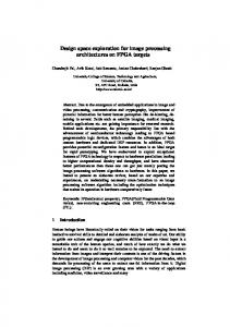
In our test, the memory of each neural architecture is computed by the LM-BP algorithm, often the fastest variant of the backpropagation algorithm and one of the most commonly used in supervised learning. The available data was split into training set, validation set, and test set, the sizes of the subcollections being 80%, 10%, and 10%, respectively. The main parameters of the LM-BP training process are specified in Table 1. In order to experimentally establish the quality of the proposed method, a comparative analysis against three of the most used and suitable algorithms for correlated noise removal, namely, BM3D (block-matching and 3D filtering [25]), NLMF (Nonlocal Means Noise Filtering [40]), and ProbShrink (correlated noise removal algorithm using nondecimated wavelet transform and generalized Laplacian [22]), was conducted. The reported results include both quantitative and qualitative comparisons. In the following, we summarize some of our results. (a) The quality evaluation of the preprocessing step in terms of the indicators (20) and (21) is as follows: (1) In Figure 1(a), a sample of five face images belonging to the Senthil database is presented, their cleaned versions resulted from applying the decorrelation and shrinkage method being shown in Figure 1(e), where each image was transmitted 30 times through the channel. In Figures 1(b), 1(c), and 1(d) the restored versions resulting from applying the NLMF algorithm, ProbShrink algorithm, and BM3D method, respectively, are depicted. Table 2 contains the
values of the indicators (20) and (21) corresponding to these five pairs of noisy-cleaned versions of these images. Note that, on average, the best results were obtained when our method was used. (2) A sample of three images of landscapes, one from each class, is presented in Figure 2(a) together with their cleaned versions resulting from applying the decorrelation and shrinkage method shown in Figure 2(e), where each image was transmitted 30 times through the channel. In Figure 2(b) the restored variants using NLMF algorithm are exhibited, while in Figure 2(c) the restored variants using ProbShrink method are shown. The cleaned version using the BM3D algorithm is presented in Figure 2(d). The values of the indicators (20) and (21) are given in Table 3. Note that, on average, the best results were obtained when our method was used. (b) As it was previously described, the images resulting from the preprocessing step are used in the supervised training of the family of neural networks. Once the training process is over, the family of neural networks are used to remove noise from new unseenyet images. Obviously, it is impossible to guarantee that the new test images share the same statistical properties with the images used during the training process, the unique criterion being that they are visually enough similar. In order to take into account this constraint, we split each of these two databases containing similar images into training and testing subsets, the sizes being 75/5 for Senthil dataset and 39/3 for the second database. (1) The test images from the Senthil database and their versions resulting from applying the preprocessing step are shown in Figures 3(a) and 3(b), respectively. Their cleaned versions computed by the resulting family of trained neural networks are shown in Figure 3(f), while their restored versions when NLMF algorithm, ProbShrink method, and BM3D method are used are presented in Figures 3(c), 3(d), and 3(e), respectively. In terms of the indicators (20) and (21), the results are summarized in Table 4. Note that in this case our method, ProbShrink algorithm, and BM3D method produce similar results, according to both SNR measure and SSIM metric.
8
Mathematical Problems in Engineering
(a)
(b)
(c)
(d)
(e)
Figure 1
(2) Similar tests were performed on the database containing images of landscapes. The tests were performed on three new images shown in Figure 4(a), the results of the preprocessing step being given in Figure 4(b). The cleaned versions computed by the resulting family of trained neural networks are shown in Figure 4(f) and the clean versions given by the BM3D algorithm are presented in Figure 4(e). The results obtained when the NLMF algorithm and ProbShrink method are used are displayed in Figures 4(c)
and 4(d), respectively. The numerical evaluation in terms of the indicators (20) and (21) is summarized in Table 5. Note that, in this case, the BM3D algorithm proved to smooth the results too much. Also, the images obtained when NLMF algorithm was used are of poor visual quality. The ProbShrink algorithm performed better than BM3D and NLMF, but, on average, the best results were obtained when our method was used.
Mathematical Problems in Engineering
9
Table 2
Noisy images versus original images Cleaned images versus original images (NLMF) Cleaned images versus original images (ProbShrink) Cleaned images versus original images (BM3D) Cleaned images versus original images (the proposed method)
SNR-RMS (the mean value)
SNR (the mean value)
Mean Peak SNR (the mean value)
SSIM (the mean value)
7.3128
17.2193
26.3217
0.5838
12.1367
21.6369
30.8944
0.8377
15.3787
23.7071
33.1043
0.8782
15.0573
23.5242
33.3160
0.8867
19.5967
25.8067
35.0112
0.9163
Table 3
Noisy images versus original images Cleaned images versus original images (NLMF) Cleaned images versus original images (ProbShrink) Cleaned images versus original images (BM3D) Cleaned images versus original images (the proposed method)
SNR-RMS (the mean value)
SNR (the mean value)
Mean Peak SNR (the mean value)
SSIM (the mean value)
7.1013
17.0083
24.6427
0.6868
7.5050
17.4992
25.8548
0.6503
9.6534
19.7858
27.7324
0.8002
8.7304
18.8084
27.6967
0.7389
20.8267
26.2779
34.0215
0.9341
(a)
(b)
(c)
(d)
(e)
Figure 2
10
Mathematical Problems in Engineering
(a)
(b)
(c)
(d)
(e)
(f)
Figure 3
Mathematical Problems in Engineering
11
Table 4 SNR-RMS/new image
SNR/new image
7.1352 7.7979 6.7452 9.0387 6.1524 8.4056 9.6450 8.3065 9.5696 7.4780 12.1067 13.6918 11.9228 14.5670 10.8248 15.6521 15.5453 14.6064 17.5242 13.2653 14.8333 16.3388 14.7108 17.7965 13.4046 13.7982 16.9576 16.5712 12.6325 13.4488
17.0681 17.8395 16.5800 19.1221 15.7809 18.4914 19.6860 18.3883 19.6179 17.4758 21.6605 22.7292 21.5275 23.2674 20.6884 23.8914 23.8320 23.2909 24.8728 22.1486 23.4248 24.2644 23.3527 25.0067 22.4632 22.7964 24.5873 24.3871 22.0298 22.5737
Noisy images versus original images
Cleaned images (using the preprocessing step) versus original images
Cleaned images versus original images (NLMF)
Cleaned images versus original images (ProbShrink)
Cleaned images versus original images (BM3D)
Cleaned images (using NN’s) versus original images (the proposed method)
Mean Peak SNR/new image 26.3356 26.4804 26.2165 26.4122 26.5486 27.8057 28.3873 28.0880 26.9517 28.2541 31.0955 31.5051 31.3547 30.6666 31.6597 33.2490 32.5356 33.0326 32.2178 33.5365 33.34 33.59 33.68 33.00 33.63 32.2178 33.0786 33.8409 29.6259 33.6427
SSIM/new image 0.5700 0.5693 0.5733 0.6410 0.5513 0.6328 0.6411 0.6392 0.6643 0.6308 0.8474 0.8448 0.8424 0.8588 0.8619 0.8834 0.8648 0.8705 0.8836 0.8812 0.8824 0.8854 0.8991 0.8525 0.9074 0.8850 0.8781 0.8968 0.8454 0.8939
Table 5
Noisy images versus original images
Cleaned images versus original images Cleaned images versus original images (NLMF) Cleaned images versus original images (ProbShrink) Cleaned images versus original images (BM3D) Cleaned images (using NN’s) versus original images (the proposed method)
SNR-RMS/new image
SNR/new image
6.7603 6.5259 7.7468 6.8194 7.8383 7.3444 7.7084 6.9041 8.2267 9.5398 9.0598 10.0007 9.0589 7.8517 9.7064 9.4599 13.1507 10.0606
16.5994 16.2928 17.7824 16.6749 17.8845 17.3191 17.7393 16.7822 18.3045 19.6813 19.1423 20.0039 19.1415 17.8993 19.7412 19.5177 22.3790 20.0525
Mean Peak SNR/new image 24.6606 24.6103 24.7497 24.7947 26.2810 24.3228 26.0425 25.3903 25.4729 27.7907 27.6171 27.5228 27.95 26.99 27.89 27.6939 30.8164 27.1269
SSIM/new image 0.6564 0.6796 0.6157 0.6590 0.7203 0.6990 0.6773 0.6025 0.6830 0.8060 0.7732 0.8218 0.7265 0.6969 0.7688 0.8090 0.8770 0.8412
12
Mathematical Problems in Engineering
(a)
(b)
(c)
(d)
(e)
(f)
Figure 4
6. Conclusive Remarks and Suggestions for Further Work The proposed method combines the decorrelation and shrinkage techniques to neural network-based approaches for noise removal purposes. The images are assumed to be transmitted as sequences of blocks of equal sizes, each block being distorted by a stationary statistical correlated noise and some amount of the noise being partially removed using the method that combines noise decorrelation and standard shrinkage technique. The preprocessing step provides, for each initial image, a sequence of blocks that are further PCAcompressed at a certain rate, each component of the resulting sequence being supplied as inputs to a feed-forward neural architecture 𝐹𝑋 → 𝐹𝐻 → 𝐹𝑌 . Therefore, each indexed block is processed by a neural network corresponding to that index value. The local memories of the neurons of the layers 𝐹𝐻 and 𝐹𝑌 are generated through a supervised learning process based on the compressed versions of blocks of the same index value supplied as inputs and the compressed versions of them resulting as the mean of their preprocessed versions. Finally, using the standard PCA-decompression technique, the sequence of the decompressed blocks is the cleaned representation of the initial image. The performance of the proposed method is evaluated by a long series of tests, the results being very encouraging as compared to similar developments for noise removal purposes. The evaluation of the amount of the noise removed is done in terms of some of the most frequently used similarity indicators, SNR, SNRRMS, Peak SNR, and SSIM.
The results produced by applying the proposed method were compared to those produced by applying three of the most widely used algorithms for eliminating correlated noise. NLMF algorithm consistently produces weaker results than the proposed method. Using ProbShrink or BM3D, the results are similar to or weaker than those yielded by the proposed method, in both quality and quantity. The long series of tests proved good results of the abovedescribed methodology entailing the hope that further and possibly more sophisticated extensions can be expected to improve it. Among several possible extensions, some work is still in progress concerning the use of different output functions for the hidden and output neurons and the use of more hidden layers in the neural architectures. Also, some other compression techniques combined with new techniques for feature extraction as well as the use of other learning schemes to generate the local memories of the neurons are expected to allow the removal of a larger amount of noise.
Competing Interests The authors declare that they have no competing interests.
Acknowledgments A major contribution to the research work reported in this paper belongs to Mrs. Luminita State, a Professor and a Ph.D. Distinguished Member of the Romanian academic
Mathematical Problems in Engineering community; Professor Luminita State passed away in January 2016. The authors will always remember her amazing spirit, as well as her brilliant mind. May God rest her soul in peace!
References [1] W. Pratt, Digital Image Processing, Wiley-Interscience, Hoboken, NJ, USA, 4th edition, 2007. [2] E. L´opez-Rubio, “Restoration of images corrupted by Gaussian and uniform impulsive noise,” Pattern Recognition, vol. 43, no. 5, pp. 1835–1846, 2010. [3] L. State, C. Cocianu, C. S˘araru, and P. Vlamos, “New approaches in image compression and noise removal,” in Proceedings of the 1st International Conference on Advances in Satellite and Space Communications (SPACOMM ’09), pp. 96–101, IEEE, Colmar, France, July 2009. [4] Z. H. Shamsi and D.-G. Kim, “Multiscale hybrid nonlocal means filtering using modified similarity measure,” Mathematical Problems in Engineering, vol. 2015, Article ID 318341, 17 pages, 2015. [5] P. Fieguth, Statistical Image Processing and Multidimensional Modeling, Springer, New York, NY, USA, 2011. [6] L. Tan and J. Jiang, Digital Signal Processing. Fundamentals and Applications, Academic Press, Elsevier, 2nd edition, 2013. [7] S. Kay, Fundamentals of Statistical Signal Processing, Volume III: Practical Algorithm Development, Prentice Hall, New York, NY, USA, 2013. [8] M. Egmont-Petersen, D. de Ridder, and H. Handels, “Image processing with neural networks—a review,” Pattern Recognition, vol. 35, no. 10, pp. 2279–2301, 2002. [9] F. Hussain and J. Jeong, “Efficient deep neural network for digital image compression employing rectified linear neurons,” Journal of Sensors, vol. 2016, Article ID 3184840, 7 pages, 2016. [10] A. J. Hussain, D. Al-Jumeily, N. Radi, and P. Lisboa, “Hybrid neural network predictive-wavelet image compression system,” Neurocomputing, vol. 151, no. 3, pp. 975–984, 2015. [11] S. Bhattacharyya, P. Pal, and S. Bhowmick, “Binary image denoising using a quantum multilayer self organizing neural network,” Applied Soft Computing Journal, vol. 24, pp. 717–729, 2014. [12] Y. Li, J. Lu, L. Wang, and Y. Takashi, “Denoising by using multineural networks for medical X-ray imaging applications,” Neurocomputing, vol. 72, no. 13–15, pp. 2884–2891, 2009. [13] I. Turkmen, “The ANN based detector to remove randomvalued impulse noise in images,” Journal of Visual Communication and Image Representation, vol. 34, pp. 28–36, 2016. [14] S. Haykin, Neural Networks A Comprehensive Foundation, Prentice Hall, 1999. [15] Y. Wu, B. H. Tracey, P. Natarajan, and J. P. Noonan, “Fast blockwise SURE shrinkage for image denoising,” Signal Processing, vol. 103, pp. 45–59, 2014. [16] A. Hyvarinen, J. Karhunen, and E. Oja, Independent Component Analysis, John Wiley & Sons, New York, NY, USA, 2001. [17] L. Shang, D.-S. Huang, C.-H. Zheng, and Z.-L. Sun, “Noise removal using a novel non-negative sparse coding shrinkage technique,” Neurocomputing, vol. 69, no. 7–9, pp. 874–877, 2006. [18] N. N. Popomarenko, V. V. Lukin, A. A. Zelensky, J. T. Astola, and J. T. Astola, “Adaptive DCT-based filtering of images corrupted by spatially correlated noise,” in Image Processing: Algorithms and Systems VI, vol. 6812 of Proceedings of SPIE, San Jose, Calif, USA, January 2008.
13 [19] N. N. Popomarenko, V. V. Lukin, K. O. Egiazarian, and J. T. Astola, “A method for blind estimation of spatially correlated noise characteristics,” in Image Processing: Algorithms and Systems VIII, vol. 7532 of Proceedings of SPIE, February 2010. [20] I. M. Johnstone and B. W. Silverman, “Wavelet threshold estimators for data with correlated noise,” Journal of the Royal Statistical Society. Series B. Methodological, vol. 59, no. 2, pp. 319– 351, 1997. [21] J. Portilla, V. Strela, M. J. Wainwright, and E. P. Simoncelli, “Image denoising using scale mixtures of Gaussians in the wavelet domain,” IEEE Transactions on Image Processing, vol. 12, no. 11, pp. 1338–1351, 2003. [22] A. Piˇzurica and W. Philips, “Estimating the probability of the presence of a signal of interest in multiresolution singleand multiband image denoising,” IEEE Transactions on Image Processing, vol. 15, no. 3, pp. 654–665, 2006. [23] B. Goossens, Q. Luong, A. Pizurica, and W. Philips, “An improved non-local denoising algorithm,” in Proceedings of the International Workshop on Local and Non-Local Approximation in Image Processing (LNLA ’08), pp. 143–156, Lausanne, Switzerland, August 2008. [24] M. Jansen, Noise Reduction by Wavelet Thresholding, Springer, Berlin, Germany, 2001. [25] K. Dabov, A. Foi, V. Katkovnik, and K. Egiazarian, “Image denoising by sparse 3-D transform-domain collaborative filtering,” IEEE Transactions on Image Processing, vol. 16, no. 8, pp. 2080–2095, 2007. [26] M. P. S. Chawla, “PCA and ICA processing methods for removal of artifacts and noise in electrocardiograms: a survey and comparison,” Applied Soft Computing Journal, vol. 11, no. 2, pp. 2216–2226, 2011. [27] L. Griffanti, G. Salimi-Khorshidi, C. F. Beckmann et al., “ICAbased artefact removal and accelerated fMRI acquisition for improved resting state network imaging,” NeuroImage, vol. 95, pp. 232–247, 2014. [28] P. Common and C. Jutten, Handbook of Blind Source Separation: Independent Component Analysis and Applications, Academic Press, Elsevier, 2010. [29] K. Fukunaga, Introduction to Statistical Pattern Recognition, Academic Press, 2nd edition, 1990. [30] J. E. Gentle, Matrix Algebra. Theory, Computations, and Applications in Statistics, Springer Texts in Statistics, Springer, New York, NY, USA, 2007. [31] I. T. Jolliffe, Principal Component Analysis, Springer Series in Statistics, Springer, Berlin, Germany, 2nd edition, 2002. [32] C. Cocianu, L. State, and P. Vlamos, “Neural implementation of a class of PCA learning algorithms,” Economic Computation and Economic Cybernetics Studies and Research no. 3/2009, 2009. [33] K. Gnana Sheela and S. N. Deepa, “Review on methods to fix number of hidden neurons in neural networks,” Mathematical Problems in Engineering, vol. 2013, Article ID 425740, 11 pages, 2013. [34] G.-B. Huang, “Learning capability and storage capacity of two-hidden-layer feedforward networks,” IEEE Transactions on Neural Networks, vol. 14, no. 2, pp. 274–281, 2003. [35] G. A. F. Seber and C. J. Wild, Nonlinear Regression, John Wiley & Sons, New York, NY, USA, 2003. [36] R. Gonzales and R. Woods, Digital Image Processing, Prentice Hall, 5th edition, 2008.
14 [37] Z. Wang, A. C. Bovik, H. R. Sheikh, and E. P. Simoncelli, “Image quality assessment: from error visibility to structural similarity,” IEEE Transactions on Image Processing, vol. 13, no. 4, pp. 600– 612, 2004. [38] http://www.geocities.ws/senthilirtt/Senthil%20Face%20 Database%20Version1. [39] http://sipi.usc.edu/database/database.php?volume=sequences. [40] A. Buades, B. Coll, and J.-M. Morel, “A non-local algorithm for image denoising,” in Proceedings of the IEEE Computer Society Conference on Computer Vision and Pattern Recognition (CVPR ’05), vol. 2, pp. 60–65, IEEE, San Diego, Calif, USA, June 2005.
Mathematical Problems in Engineering
Advances in
Operations Research Hindawi Publishing Corporation http://www.hindawi.com
Volume 2014
Advances in
Decision Sciences Hindawi Publishing Corporation http://www.hindawi.com
Volume 2014
Journal of
Applied Mathematics
Algebra
Hindawi Publishing Corporation http://www.hindawi.com
Hindawi Publishing Corporation http://www.hindawi.com
Volume 2014
Journal of
Probability and Statistics Volume 2014
The Scientific World Journal Hindawi Publishing Corporation http://www.hindawi.com
Hindawi Publishing Corporation http://www.hindawi.com
Volume 2014
International Journal of
Differential Equations Hindawi Publishing Corporation http://www.hindawi.com
Volume 2014
Volume 2014
Submit your manuscripts at http://www.hindawi.com International Journal of
Advances in
Combinatorics Hindawi Publishing Corporation http://www.hindawi.com
Mathematical Physics Hindawi Publishing Corporation http://www.hindawi.com
Volume 2014
Journal of
Complex Analysis Hindawi Publishing Corporation http://www.hindawi.com
Volume 2014
International Journal of Mathematics and Mathematical Sciences
Mathematical Problems in Engineering
Journal of
Mathematics Hindawi Publishing Corporation http://www.hindawi.com
Volume 2014
Hindawi Publishing Corporation http://www.hindawi.com
Volume 2014
Volume 2014
Hindawi Publishing Corporation http://www.hindawi.com
Volume 2014
Discrete Mathematics
Journal of
Volume 2014
Hindawi Publishing Corporation http://www.hindawi.com
Discrete Dynamics in Nature and Society
Journal of
Function Spaces Hindawi Publishing Corporation http://www.hindawi.com
Abstract and Applied Analysis
Volume 2014
Hindawi Publishing Corporation http://www.hindawi.com
Volume 2014
Hindawi Publishing Corporation http://www.hindawi.com
Volume 2014
International Journal of
Journal of
Stochastic Analysis
Optimization
Hindawi Publishing Corporation http://www.hindawi.com
Hindawi Publishing Corporation http://www.hindawi.com
Volume 2014
Volume 2014