Neural Architectures for Unifying Brightness Perception and Image ...

Neural Architectures for Unifying Brightness Perception and Image Processing

´ Instituto de Optica (CSIC) Image and Vision Department Serrano 121, E-28006 Madrid (Spain) and Abteilung Neuroinformatik Fakult¨ at f¨ ur Informatik Universit¨ at Ulm Albert-Einstein-Allee, D-89069 Ulm (Germany)

Dissertation zur Erlangung des Doktorgrades Dr.rer.nat. der Fakult¨ at f¨ ur Informatik der Universit¨ at Ulm

Matthias Sven Keil aus Hof an der Saale (erschienen 2002)

Amtierender Dekan:

Prof. Dr. F. W. von Henke

Gutachter 1:

Prof. Dr. Heiko Neumann

Gutachter 2:

Prof. Dr. G¨ unther Palm

Gutachter 3:

Dr. Gabriel Crist` obal

Tag der Promotion:

16. Juni 2003

Contents 1 Biophysical Principles 1.1 Biological neurons and the equivalent circuit . . . . . . . . . . . . . 1.2 The membrane equation of a passive neuron . . . . . . . . . . . . . 1.2.1 Synaptic input . . . . . . . . . . . . . . . . . . . . . . . . . 1.3 Realistic vs. abstract modeling of biological neurons . . . . . . . . 1.3.1 Spike rate vs. mean firing rate . . . . . . . . . . . . . . . . 1.3.2 Driving Potential vs. Potential-Independent Synaptic Input 1.4 Dendrites . . . . . . . . . . . . . . . . . . . . . . . . . . . . . . . . 1.5 Summary . . . . . . . . . . . . . . . . . . . . . . . . . . . . . . . .

. . . . . . . .

2 An Introduction to Brightness Perception 2.1 Luminance, brightness, and the visual pathway . . . . . . . . . . . . 2.2 Retinal Ganglion cells constitute the retinal output . . . . . . . . . . 2.2.1 Retinal ganglion cells respond to luminance contrasts . . . . 2.2.2 The difference-of-Gaussian (DOG) model . . . . . . . . . . . 2.2.3 Nonlinearly summing ganglion cells . . . . . . . . . . . . . . . 2.2.4 Ganglion cells in the primate retina . . . . . . . . . . . . . . 2.3 Beyond the retina - cortical representations of surfaces . . . . . . . . 2.3.1 Viewing brightness perception as a coding problem . . . . . . 2.3.2 Cortical surface representations . . . . . . . . . . . . . . . . . 2.3.3 Creating surface representations - the filling-in hypothesis . . 2.3.4 Neurophysiological correlate for filling-in . . . . . . . . . . . . 2.3.5 Filling-in models of brightness perception . . . . . . . . . . . 2.3.6 Formal description of standard filling-in . . . . . . . . . . . . 2.3.7 Filling-in and inverse problems . . . . . . . . . . . . . . . . . 2.3.8 Standard filling-in is a special case of confidence-based filling-in 2.4 Models for brightness perception and the anchoring problem . . . . . 2.4.1 An extra luminance-driven or low-pass channel . . . . . . . . 2.4.2 Superimposing band-pass filters . . . . . . . . . . . . . . . . . 2.4.3 Directional filling-in (1-D) . . . . . . . . . . . . . . . . . . . . 2.4.4 The multiplexed retinal code - a novel approach . . . . . . . 2.5 Summary . . . . . . . . . . . . . . . . . . . . . . . . . . . . . . . . .

2

6 6 7 9 13 13 14 15 18 20 21 22 22 22 23 23 26 26 26 27 29 30 32 32 34 34 35 37 39 39 40

3 Novel Retinal Models 3.1 Introduction . . . . . . . . . . . . . . . . . . . . . . . . . . . . . . . . 3.2 The luminance correlation coefficient (LCC) . . . . . . . . . . . . . . 3.3 The standard model of retinal ganglion cells . . . . . . . . . . . . . . 3.3.1 Differential equations for the membrane potential . . . . . . . 3.3.2 Steady-state solutions . . . . . . . . . . . . . . . . . . . . . . 3.3.3 Choice of receptive field parameter . . . . . . . . . . . . . . . 3.3.4 Positions of retinal responses relative to luminance discontinuities . . . . . . . . . . . . . . . . . . . . . . . . . . . . 3.3.5 Luminance correlation coefficient with the standard model . . 3.4 How luminance information may be passed into the cortex . . . . . . 3.4.1 Neurophysiological evidence - the extensive disinhibitory surround (DIR) . . . . . . . . . . . . . . . . . . . . . . . . . . . 3.4.2 Incorporating the three-Gaussian model into the standard retinal model . . . . . . . . . . . . . . . . . . . . . . . . . . . 3.5 Novel retinal models - multiplexing contrast and luminance in parallel channels . . . . . . . . . . . . . . . . . . . . . . . . . . . . . . . . . . 3.5.1 A novel model for retinal ganglion cells . . . . . . . . . . . . 3.5.2 Model I - divisive gain control . . . . . . . . . . . . . . . . . . 3.5.3 Model II - multiplicative gain control . . . . . . . . . . . . . . 3.5.4 Improving the modulation depth of the multiplicative gain control . . . . . . . . . . . . . . . . . . . . . . . . . . . . . . . 3.5.5 Model III - saturating multiplicative gain control . . . . . . . 3.6 Summary . . . . . . . . . . . . . . . . . . . . . . . . . . . . . . . . .

41 41 42 43 43 44 45

4 A New Role for Even Simple Cells 4.1 A brief overview of the proposed architecture . . . . . 4.2 Formal description of the texture system . . . . . . . . 4.2.1 Orientation selectivity as quasi one dimensional 4.2.2 Detecting even symmetric features (“texture”) 4.3 Results and discussion . . . . . . . . . . . . . . . . . .

. . . . .

65 65 67 67 70 75

. . . . . . . . . . .

79 79 80 84 85 85 86 86 88 89 90 93

. . . . . . . . . . . . . . framework . . . . . . . . . . . . . .

5 A Novel Nonlinear Filling-in Framework 5.1 Introduction . . . . . . . . . . . . . . . . . . . . . . . . . . 5.1.1 Limitations of Filling-in . . . . . . . . . . . . . . . 5.2 Detecting odd symmetric features . . . . . . . . . . . . . . 5.2.1 Excitatory input into an odd symmetric simple cell 5.2.2 Inhibitory input into an odd symmetric simple cell 5.2.3 Odd symmetric cell . . . . . . . . . . . . . . . . . . 5.3 Gating of multiplexed activity by odd-cell activity . . . . 5.3.1 Combination of orientation channels . . . . . . . . 5.4 Generalized diffusion operators . . . . . . . . . . . . . . . 5.5 BEATS filling-in diffusion layer . . . . . . . . . . . . . . . 5.6 Exploring the parameter space for surface syncytia . . . .

. . . . . . . . . . .

. . . . . . . . . . .

. . . . . . . . . . .

. . . . . . . . . . .

. . . . . . . . . . .

46 48 49 49 50 52 53 56 59 61 62 63

4

5.7

5.8 5.9

Simulations of brightness illusions . . . . . . . . 5.7.1 Craik-O’Brien-Cornsweet effect (COCE) 5.7.2 Grating induction . . . . . . . . . . . . 5.7.3 Chevreul’s illusion . . . . . . . . . . . . 5.7.4 A modified Chevreul illusion . . . . . . 5.7.5 Simultaneous brightness contrast . . . . 5.7.6 White’s effect (Munker-White effect) . . 5.7.7 Benary cross . . . . . . . . . . . . . . . 5.7.8 The Hermann/Hering grid . . . . . . . . 5.7.9 The scintillating grid illusion . . . . . . Surface representations with real-world images Summary . . . . . . . . . . . . . . . . . . . . .

. . . . . . . . . . . .

. . . . . . . . . . . .

. . . . . . . . . . . .

. . . . . . . . . . . .

. . . . . . . . . . . .

. . . . . . . . . . . .

6 Recovering luminance gradients 6.1 Introduction . . . . . . . . . . . . . . . . . . . . . . . . . . 6.2 Formal description of the gradient system . . . . . . . . . 6.2.1 Detecting linear and nonlinear luminance gradients 6.2.2 Recovering luminance gradients . . . . . . . . . . . 6.3 Simulations of brightness illusions . . . . . . . . . . . . . . 6.3.1 Mach bands . . . . . . . . . . . . . . . . . . . . . . 6.3.2 Sine wave gratings and Gabor patches . . . . . . . 6.4 Simulations with real-world images . . . . . . . . . . . . . 6.4.1 Varying the feature inhibition weight . . . . . . . . 6.5 Summary . . . . . . . . . . . . . . . . . . . . . . . . . . .

. . . . . . . . . . . .

. . . . . . . . . .

. . . . . . . . . . . .

. . . . . . . . . .

. . . . . . . . . . . .

. . . . . . . . . .

. . . . . . . . . . . .

. . . . . . . . . .

. . . . . . . . . . . .

. . . . . . . . . .

. . . . . . . . . . . .

97 97 99 106 108 109 111 114 116 118 118 129

. . . . . . . . . .

132 132 133 133 135 139 139 147 147 149 150

7 Binding of surfaces, texture, and gradients 161 7.1 Combining maps computationally . . . . . . . . . . . . . . . . . . . . 161 7.2 Combining maps in the brain . . . . . . . . . . . . . . . . . . . . . . 162 8 Zusammenfassung (in German)

164

A Nonlinear A.0.1 A.0.2 A.0.3

166 166 167

Diffusion Introduction . . . . . . . . . . . . . . . . . . . . . . . . . . . Formal Description . . . . . . . . . . . . . . . . . . . . . . . . Global normalization by local interactions (dynamic normalization) . . . . . . . . . . . . . . . . . . . . . . . . . . . . . . A.0.4 Nonlinear contrast extraction . . . . . . . . . . . . . . . . . . A.0.5 Could dynamic normalization account for brightness phenomena? . . . . . . . . . . . . . . . . . . . . . . . . . . . . . . . . A.0.6 Discussion . . . . . . . . . . . . . . . . . . . . . . . . . . . . .

173 176 180 189

An overview The architecture for brightness processing proposed with the present work aims to unify two seemingly diverging goals, that is image processing and brightness perception. A successful unification has not been achieved so far, since models which predict brightness phenomena only rarely produce meaningful results when processing real-world images (although some results have been demonstrated, e.g. [Sepp & Neumann, 1999]). On the other hand, models for image processing tasks (typically coding or denoising), which often claim to provide some account to early vision, fail to predict phenomena associated with brightness perception. Usually, both model classes compute their output by superimposing processed filter outputs over various scales and orientations, whereby filter outputs are processed in order to fulfill a certain pre-defined goal (coding, denoising, predicting psychophysical results, etc.). None of these models has achieved any segregation of the visual input in way compatible with object recognition; rather, these models create only an internal (or cortical) representation of the visual input, thus deferring segregation mechanisms to higher level cortical processing. Furthermore, there is no model available for processing two-dimensional luminance patterns which comes up with a neurophysiological plausible solution to the anchoring problem (although a one-dimensional solution was suggested by [Arrington, 1996]). This problem is commonly solved by employing an additional “luminance channel” in the form of a low-passed filtered (or large-scale band-passed, e.g. [Sepp & Neumann, 1999]) version of the visual input, e.g. [Pessoa et al., 1995, du Buf & Fischer, 1995, Neumann, 1996, McArthur & Moulden, 1999, Blakeslee & McCourt, 1999]. Yet, evidence supporting the existence of such a channel is still lacking. In this thesis a novel architecture for foveal brightness perception is presented in agreement with both neurophysiological and psychophysical data (see figure 4.1 on page 65). It is proposed that cortical simple cells of different symmetries (even, odd) and sizes extract different aspects from the visual input, which are (i) texture (here defined as small-scale even symmetric features, such as lines and points, chapter 4), (ii) surfaces (corresponding to small-scale odd symmetric features for building cortical surface representations, chapter 5), and (iii) luminance gradients (corresponding to large-scale even and odd symmetric features, for example out-of-focus lines or edges, chapter 6). Simulations show how this segregation process renders cortical representations of object surfaces invariant to noise and illumination gradients. Also, a neurophysiologically plausible solution to the anchoring problem is suggested by proposing a “multiplexed” retinal code which at the same time represents information about contrast and brightness (ON-cell) and contrast and darkness (OFF-cell) of a visual input (chapter 3). The architecture builds upon filling-in theory [Gerrits & Vendrik, 1970, Grossberg & Todorović, 1988]. In the present work, however, filling-in is implemented with a novel nonlinear diffusion paradigm (“BEATS” filling-in), instead of using a linear diffusion mechanism as it is normally the case (nonlinear diffusion is presented and analyzed in appendix A).

5

Chapter 1

Biophysical Principles This chapter gives a concise introduction into the biophysical concepts of neurons. The equation for the description of a neuron’s membrane potential is derived, which serves as a “working horse” for the computational modeling level which is used in subsequent chapters. Thus, this chapter examines the interplay between the biophysical level of description (low and detailed), and the computational level of description (higher, but more abstract). Above all, the following questions will be addressed: (i) What computations can be carried out by biological neurons? This endows us with a set of biophysically plausible mathematical operations on the computational description level. (ii) Which description level should be chosen for our purposes? It certainly makes no sense to model ionic channels, dendritic compartments, etc. Rather, on a computational level, these details are approximated by corresponding mathematical operations. (iii) Under which conditions does a simplified description of a neuron yield biological plausible results? This question addresses the interplay between biophysical details on the one hand and an adequate formulation on the computational level of description on the other. As it will turn out, these questions can not be answered independently. This chapter builds to a large extent on the books of [Koch, 1999] and [Kandel et al., 2000].

1.1

Biological neurons and the equivalent circuit

In a crude picture, a biological neuron consists of a soma endowed with neurites (dendrites and axons). The dendrite usually collects information from within a volume, where it makes connections to axons of other neurons. Axons may be seen as the output channel of a neuron. Connections between different neurons are made through special structures, called synapses (see below). The quantity which describes the state of our model neurons corresponds to the biophysical membrane potential. The membrane potential of a cortical neuron is defined as the difference between the intracellular and the extracellular potential at a certain time. This difference exists because a cell membrane separates the cytoplasm from ionic solutions in extracellular space. Usually, these solutions differ in their respective concentrations of ionic charges. If no signaling takes place, and the neuron’s membrane potential remains constant over time, then the membrane potential is said to be at its resting value. Because the extracellular potential is, by convention, defined as zero, the neuron’s inside resting potential falls usually into the range between −70mV and −60mV. If we had a passive membrane, the resting potential of an ionic species would be determined by two counterbalancing forces. On the one hand, a chemical driving

6

CHAPTER 1. BIOPHYSICAL PRINCIPLES

7

force (which depends on the concentration gradient across the membrane) would act to make ion concentrations on either side of the cell membrane homogeneous by means of diffusion. Diffusion takes place over ion specific resting membrane channels. These channels are always opened irrespective of the current value of the membrane potential. On the other hand ions “see” an electrical driving force which would counteract diffusion. This electrical force depends on the degree of polarization of the cell membrane. Summarizing: ion flux = membrane conductance × (electrical driving force + chemical driving force)

The neuronal resting potential actually derives from a dynamical equilibrium, since active (i.e. energy consuming) processes keep the ionic gradients from reaching their thermodynamical equilibrium. For example, the sodium-potassium pump maintains the electrochemical gradients of N a+ and K + by hydrolysis of one ATP molecule1 to export three N a+ cations from, and to import two K + cations into the neuron. The effect is a decrease of the membrane potential compared to its value at thermodynamical equilibrium (i.e. the absence of ionic gradients). In a dynamic scenario a neuron can be modeled with an electrical circuit, called the equivalent circuit. In the equivalent circuit, ion channels are represented by resistors and conductors, respectively, corresponding to electrical driving forces. Concentration gradients (i.e. the chemical driving forces) are represented by fictive batteries. An ion channel is described by a conductor in series with a battery. Finally, the polarization of the cell membrane (which is made up of two layers of phospholipid 2 molecules) is described by a capacitor.

1.2

The membrane equation of a passive neuron

In the absence of any concentration gradient (i.e. no diffusion takes place), the current through a channel is described by Ohm’s law: I = g × V m where g is the total conductance (=1/resistance R) of all channels of a specific type (g = number of channels × conductance of an individual channel). V m is the membrane potential. In the presence of a concentration gradient, however, in addition the corresponding chemical driving force must be taken into account. In the equivalent circuit, the chemical driving force for each ion is represented by a battery, whose electromotoric force is independent of the number of ion channels, but depends only on the concentration gradient. Thus, the battery’s electromotive 3 force is given by the Nernst potential (i.e. the equilibrium potential) E for that ion 4 , which is proportional to its logarithm of inside-to-outside concentration ratio. Electrical and chemical driving forces act in opposed directions, i.e. I = g × (V m − E). The negative sign is defined by convention. Consequently, the electrochemical driving force or driving potential across the channel is represented by the term Vm − E. The ionic charges Q which accumulate on the inside and the outside of the cell membrane give rise to a potential difference Vm over the cell membrane: Q = C×Vm . If we assume the capacity C to be constant over the cell membrane, then we obtain for some resting channel (by calculating I = dQ/dt) 1

Adenosine triphosphate or ATP is an important energy source for biological processes. any of numerous lipids (as lecithins and phosphatidylethanolamines) in which phosphoric acid as well as a fatty acid is esterified to glycerol, and which are found in all living cells, and in the bilayers of plasma membranes. 3 something that moves or tends to move electricity: the potential difference derived from an electrical source per unit quantity of electricity passing through the source (such as a cell or generator). 4 e.g. EK + = −75 mV, EN a+ = +55 mV, EC l− = −60 mV 2


8

Figure 1.1: Equivalent circuit. (A) A sketch of the lipid bilayer membrane of a passive neuron with embedded resting ion channels. (B) Corresponding effective equivalent circuit, as described by equation 1.2. (Reprinted without any permission from [Hille, 1992, Koch, 1999])

C

dVm (t) = g × (E − Vm ) dt

(1.1)

In reality there is no flow any (capacitive) current over the lipid bilayer of the membrane, since it is an insulator. Rather, the last equation should be interpreted as a redistribution of ionic charges over time, as a consequence of ion flux over the channels embedded in the membrane5 : rapid changes in voltage are associated with large capacitive currents. The complete equivalent circuit consists of various channel types (e.g. potassium, sodium and chloride), two extra current sources for the N a + -K + pump, and a capacitor. However, we can lump together these channels and the ionic pump into an effective conductance, called the leakage conductance or decay constant g leak . This follows from the fact that the conductance of the individual resting channels does not change as function of membrane potential. Furthermore, the electrogenesis 6 due to the N a+ -K + pump is small, so it may be neglected. Then, we can express the passive properties of the neuron as deviation from its resting potential V rest C

dVm (t) = gleak × (Vrest − Vm ) dt

(1.2)

Equation 1.2 describes the effective equivalent circuit shown in figure 1.1. The “reaction-time” of the passive neuron is characterized by the time constant τ = C/gleak , which describes the time to charge an isopotential patch of membrane to the 1/e part of its steady-state value. Imagine that we initialize V m with some value and subsequently monitor Vm with time. If gleak is big, then Vm will quickly approach Vrest . This endows the neuron with a high temporal resolution (τ from 1 to 2 msec as typical values). For relatively slow neurons, τ may be as big as 100 msec. Moreover, it is known that the conductivity of the potassium resting channel is not fixed, but may be modulated by so-called neuromodulators, such as acetylcholine (ACh). 5 The presence of resting ion channels increases a neuron’s membrane conductance by a factor of about 40000 compared to the case without channels in the cell membrane. 6 The production of electrical activity in living tissue.


1.2.1

9

Synaptic input

Neurons are interconnected via synapses, of which two general types are known. Chemical synapses separate the cytoplasm of two neurons by a synaptic cleft, and transmission of information proceeds in one distinct direction. Hence, we have an input or presynaptic site, and an output or postsynaptic site. Electrical synapses (or gap junctions) on the other hand establish cytoplasmic continuity between preand postsynaptic cells. They usually operate bidirectionally. Gap junctions provide a “high-conductance pathway” for the instantaneous exchange of ionic currents between adjacent neurons. Additionally, the strength of coupling between gap junction channels can be modulated by, for example, the intracellular concentration of calcium ions, or the cytoplasmic pH value [Bennett & Spray, 1987]. Most gap-junction channels close whenever the pH is low or the C a 2+ concentration is high. Another source for modulating the conductivity of gap-junction channels are neurotransmitters released by nearby chemical synapses. Moreover, there exist specialized gap junctions endowed with voltage-dependent channels [Edwards et al., 1991, Edwards et al., 1998]). These so-called rectifying gap junctions conduct depolarizing currents only in one direction. Transmission of signals by chemical synapses involves a significant delay (called latency) by at least 0.3 msec from the pre- to the postsynaptic site, but longer delays which range from 1 to 5 msec are more typical. The reason for the latency is that an electrical signal which arrives at a chemical synapse must be converted into a chemical messenger, consisting of a neurotransmitter (transmitting step). The neurotransmitter subsequently diffuses 20 to 40 nm over the synaptic cleft. On the postsynaptic site, neurotransmitters act like a “key” which must fit into the “lock” (the receptor molecule) in order to open or close the associated “gate” (the ionic channel). The resulting ion flux alters the membrane conductance and potential of the postsynaptic cell. The value by which the membrane potential changes is called the postsynaptic potential (PSP). Postsynaptic potentials (PSPs) come in two different flavors: excitatory (EPSPs) and inhibitory (IPSPs). IPSPs increase the polarization relative to rest. This so-called hyperpolarization leads thus to a more negative membrane potential. Conversely, depolarization refers to a more positive membrane potential as a consequence of EPSPs impinging on the neuron. If depolarizing current pulses manage it to increase the membrane potential over some threshold value, then voltage-gated ion channels will open. This triggers a cascade a biophysical events in a somatic zone called the axon hill-lock, culminating in the generation of binary events called action potentials or spikes. The spikes then travel down the axon, and their dissipation is prevented by active regeneration mechanism embedded in the axon. This corresponds to the “output” information or response delivered to other neurons. A confirmation signal for active dendritic synapses is provided by means of backpropagating action potentials, which may induce long term potentiation if pre- and postsynaptic cells fire within some time window, or long term depression if pre- and postsynaptic cell fire asynchronously 7 [Holmgren & Zilberter, 2001] (see also footnote 1 on page 162). Below a neuron’s firing threshold does the membrane respond only passively with so called electrotonic8 potentials. A presynaptic cell has to fire before information transmission with chemical synapses can take place. This stands in contrast to most electrical synapses, which can trans7 Long term potentiation refers to strengthening of the synaptic weight, whereas long term depression leads to a reduction in the synapse’s effectivity. This essentially corresponds to Hebbian and anti-Hebbian learning, respectively [Hebb, 1949]. 8 The spread of electrical activity through living tissue or cells in the absence of repeated action potentials.


10

mit both subthreshold hyperpolarizing and subthreshold depolarizing currents. The latter property is referred to as electrotonic transmission. How should PSPs mathematically be treated? The principal effect of the release of neurotransmitter from the synapse’s active zone is an increase in the conductance of the postsynaptic cell membrane for some specific ion type. This change in conductance implies an ionic flux. Since currents add, we can generalize equation 1.2 in a straightforward manner to n

C

X dVm (t) = gleak (Vrest − Vm ) + gsyn,i (t)(Esyn,i − Vm ) dt i=0

(1.3)

where n denotes the number of synapses, and gsyn,i (t) is the (usually time dependent) change in the conductance of the cell membrane, due to the opening of specific ion channels. Esyn,i is called reversal potential or synaptic battery of the synapse, which is associated with a specific ion type. A two dimensional layer of neurons where adjacent neurons are coupled via electrical synapses (called a syncytium9 ) can be modeled by a reaction-diffusion systems (e.g. [Winfree, 1995]). The diffusion part derives from the one dimensional cable equation, which describes the spread of potentials (the cable equation was originally devised for submarine telegraph cables). The reaction part of the reaction-diffusion system describes the response of the cell membrane to the flow of ionic current: C

dVm (t) = gleak (Vrest − Vm ) + D∇2 Vm dt

(1.4)

D denotes the constant diffusion coefficient indicating the speed of activity propagation; in the myocardium (the middle muscular layer of the heart wall) D ≈ 1cm 2 /s. With chemical synapses we can distinguish three effects when an ion channel opens, depending on the value of the corresponding synaptic batteries relative to the cell’s resting potential. With (i) Esyn,i > Vrest an inward (i.e. negative) flux of ions takes place. The effect on the membrane potential will be excitatory, and an EPSP is produced. Excitatory receptors are activated by the neurotransmitter glutamate. Among these, there are three major subtypes, which are distinguished by synthetic agonists 10 : AMPA11 , kainate, and NMDA12 . Fast excitation is mediated by the AMPA and kainate receptors, which are sometimes also called non-NMDA receptors. The NMDA receptor has some outstanding properties13 , in that it requires the presence of glutamate and at the same time the depolarization of the cell in order to open. 9 Normally a syncytia is defined as a a multinucleate mass of protoplasm resulting from fusion of cells. Grossberg [Grossberg & Todorović, 1988] refers to it as a regular array of intimately connected cells such that contiguous cells can easily pass signals between each other’s compartment membranes, possible via gap-junctions. Syncytia and their corresponding reaction-diffusion equations will be heavily used throughout the thesis. 10 A chemical substance capable of combining with a receptor on a cell and initiating a reaction or activity. 11 α-amino-3-hydroxy-5-methylisoxazole-4-propionic acid 12 N-methyl-D-aspartic acid 13 (i) The associated cation channel has a high conductivity. The channel is permeable to C a2+ as well as K + and N a+ . (ii) Opening the channel requires an additional substance (a cofactor), namely glycine, which normally is present in sufficient concentration in the extracellular fluid. (iii) In addition, opening requires a “plug” to be removed from the channel (the plug prevents the flow of ionic currents). This plug consists of a M g 2+ cation, which is expulsed at sufficiently high depolarization. Otherwise expressed, the channel opens in a voltage-dependent fashion.


11

With Esyn,i ≤ Vrest the current is directed outward and gives rise to an IPSP. This implies the hyperpolarization of the cell membrane. IPSPs of most central neurons are mediated by the neurotransmitter GABA14 . GABA is effective on two receptors, which are GABAA and GABAB . GABAA mediated inhibition is fast because it acts directly (ionotropically) on the C l − channel. Its reversal potential is close to the cell’s resting potential. Opening of a GABAA gated channel at Vm ≈ Esyn,GABAA increases merely the membrane conductance (while decreasing the membrane time constant τ from τ ≡ C/gleak to τ ≈ C/(gleak + gsyn,GABAA ) where gsyn,GABAA > 0). As long as the membrane potential is not driven away from its resting value, this form of inhibition remains silent because no active hyperpolarization of the cell takes place. With a depolarized neuron, however, GABAA inhibition blows its cover and, in addition to the passive decay, shunts or short-circuits the membrane potential to the “extracellular ground”. Thus, when (ii) Esyn,i ≈ Vrest , we speak of silent or shunting inhibition. GABAB mediated inhibition, on the other hand, acts more slowly due to its indirect (metabotropical) gating of a K + mediated channel through a second-messenger cascade. The corresponding reversal potential is quite far from the cell’s resting potential, that is Esyn,i < Vrest (case (iii) ), leading to a more subtractive type of inhibition. After the activation of a GABAB gated channel, the cell’s membrane potential will decrease. Note that each synaptic input (whether excitatory, inhibitory or shunting) decreases the membrane time constant by increasing the synaptic input conductance. This can be understood by inspection of equation 1.3. By considering the change of the membrane potential relative to rest V ≡ Vm − Vrest and by rearranging terms we obtain # " n n X X dV (t) C gsyn,i (t)(Vrest − Esyn,i ) gsyn,i (t) + = −V gleak + dt i=0 i=0

(1.5)

For slowly varying synaptic input, we can consider each of the g syn,i (t) as approximately constant. Then we may define an effective membrane time constant τ eff as τeff := τ / 1 +

1 gleak

n X

gsyn,i

i=0

!

(1.6)

Thus, the passive membrane time constant τ ≡ C/gleak is rescaled by a factor which decreases as the synaptic input increases. This holds true for any type of synaptic input i, since τeff does not depend on any specific reversal potential E syn,i . Because the overall membrane conductance is changed by any synaptic input, we may express the effective membrane conductance geff as geff := gleak +

n X

gsyn,i

(1.7)

i=0

By using the definitions for both τeff and geff we can rewrite equation 1.5 into the compact form (remember that gsyn,i (t) ≈ const ∀i) τeff 14

n 1 X dV (t) = −V + gsyn,i (Esyn,i − Vrest ) dt geff i=0

γ-aminobutyric acid

(1.8)


2

12

3

gGABA−A input 1.5

0 10 100 1000

2.5

gGABA−A input

2

∞

max(V ,0)

1

V∞

0.5

0

0 10 100 1000

1.5

1 −0.5 0.5

−1

−1.5

0

10

20

30

40

50

60

70

80

90

100

gsyn,AMPA

0

0

100

200

300

400

500

600

700

800

900

1000

gsyn,AMPA

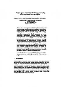
Figure 1.2: Saturating of steady state potential V∞ with excitatory (i.e. AMPAlike) synaptic input. Units are arbitrary, according to the re-scaling procedure described with table 1.1. Left: Plot of steady-state potential V∞ (equation 1.10 with values of table 1.1) in the presence of different amounts of constant inhibitory GABAA synaptic input. In the essence, increasing gsyn,GABAA acts to increase the leakage conductance of the cell membrane since Vrest ≈ Esyn,GABAA . In the presence of strong GABAA -mediated shunting inhibition, the effective leakage conductance gleak + gsyn,GABAA renders the much more smaller excitatory synaptic input gsyn,AMPA insignificant. This leads to a more linear transfer function. Right: Same scenario as with the left plot, but now showing the suprathreshold generator potential over a bigger range of excitatory input. With bigger effective leakage conductances the neuron needs to be excited more to get active (i.e. to fulfill Vm ≥ Vth ). The last equation has the general solution

V (t) =

1 geff

"

n X i=0

#

gsyn,i (Esyn,i − Vrest ) · 1 − e−t/τeff

(1.9)

The potential V (t) converges for t→∞ to its steady-state value V ∞

V∞ =

Pn

(Esyn,i − Vrest ) i=0 gsyn,i P n gleak + i=0 gsyn,i

(1.10)

The last equation gives rise to several interesting insights. First, if V rest = Esyn,j for some synaptic input j, then the corresponding term g syn,j (Esyn,j −Vrest ) in the sum of the numerator will vanish. But there is still a contribution g syn,j left in the sum of the denominator that diminishes V∞ in a divisive manner. For this reason shunting inhibition is sometimes also referred to as divisive inhibition [Bloomfield, 1974]. Second, regardless of the nature of synaptic input (excitatory or inhibitory), each input gives rise to a divisive component in the membrane potential. This characteristic gives rise to a “self-normalizing” behavior [Grossberg, 1983]. The input-output characteristic for the single voltage compartment, is called transfer or signal function. Figure 1.2 shows that this curve saturates with high excitatory input. This means that the dynamic range of the input is compressed: the original dynamic range of the synaptic input is mapped onto a smaller output range.


1.3 1.3.1

13

Realistic vs. abstract modeling of biological neurons Spike rate vs. mean firing rate

Neurons which are modeled in this work are not endowed with a spike generator. As long as the membrane potential stays subthreshold (V m < Vth ), ignoring the spiking mechanism is not at odds with biological neurons, because it remains inactive. If Vm ≥ Vth , then biological neurons will fire action potentials (or spikes). Each single spike is followed by a variable reset (or EPSP shunting) of synaptic integration [H¨ aussler et al., 2001]. The magnitude of EPSP shunting depends on the relative timing between an action potential and subsequently arriving EPSPs. It depends furthermore on the location of the synapse on the dendritic tree (since EPSP shunting due to spiking seems only effective within a distance of 300 µm from the soma). The firing of an action potential is followed by a refractory period 15 . If we pharmacologically blocked, for instance, the fast sodium conductances ([Koch, 1999], chapter 14), we would be able to directly monitor the generator potential, that is the somatic potential with a disabled spiking mechanism. A common praxis to compute the firing rate from the above-threshold membrane potential V ≡ max(Vm , 0) is to apply some continuous monotonic function g, i.e. f= g(V ). Popular choices are, for example, a sigmoidal function f=1/(1+exp(−2βV )) with β>0, f ∝V 2 [Grossberg, 1973, Heeger et al., 1996, Carandini et al., 1997], or f=tanh(V ) [Hopfield, 1984]. In many models of neurons without active spiking mechanism the assumption is made that the generator potential is equal to the mean or average firing rate. The mean firing rate is usually computed by presenting an animal several times an (in space and time) identical stimulus while monitoring the output of a neuron for which this stimulus is effective. The spikes which are generated by the stimulus are thereby recorded over a time window which should be large in comparison to the variation time of the sensory stimulus. This ensures that any observed variation in the output of the monitored neuron is not due to the stimulus. Averaging the output over stimulus trials gives an estimation of the mean firing rate. However, generator potential and (mean) firing rate are correlated only up to a certain point in biological neurons (see [Koch, 1999], chapter 14.3 with references), and inactivation of the spike generator has implications for modeling. First, a spiking mechanism can speed up a neuron’s response. How? Assume that we increase τ ≡ C/gleak , e.g. by decreasing gleak . This will also increase the rate of voltage change dVdt(t) . Up to the neuron’s firing threshold Vth there is no difference between a neuron with an active and an inactive spiking mechanism: a step-like input into both neurons causes the slope of the V (t) curve to increase. However, when a spike is fired, then the action potential is reset to ≈ V rest , and the neuron charges up again and so on. In other words, the spiking neuron has reached its (dynamical) equilibrium. However, a steeper V (t) curve for a neuron with disabled spiking mechanism means that it takes even longer to reach its steady-state (or equilibrium) potential. For a spiking neuron, on the other hand, it means that a steeper slope of V (t) causes it to fire the first spike more rapidly compared with lower values of τ . In this way the spiking mechanism speeds up the time to reach the equilibrium potential, at least for a current step injection. Second, shunting inhibition can have two different effects in the presence of a spiking mechanism: divisive in the subthreshold domain (Vm < Vth ), but subtractive in the suprathreshold domain (Vm ≥ Vth ) [Holt & Koch, 1997, Holt, 1998]. For Vm< Vth , shunting inhibition can be considered as merely increasing the leakage conductance gleak (cf. figure 1.2). The effect thus is divisive (cf. equation 1.10). 15 This is a period of diminished excitability after an action potential was fired, due to residual inactivation of N a+ channels and increased opening of K + channels.


14

For Vm ≥ Vth , however, a spike is triggered which subsequently resets the membrane potential to its resting value Vrest . This implies that, no matter how large the synaptic input currents Isyn are, the overall current over the membrane has the upper bound Vth geff (compared to Isyn /geff without spiking mechanism). As a consequence of the existence of such an upper bound it can be shown that the firing rate is decreased in a subtractive manner, especially when the inhibition is located at or very close to the soma on the dendritic tree (see [Koch, 1999], chapter 18.5 with references). Nevertheless, if shunting inhibition acts on the more distal part of the dendrite, its divisive character seems to dominate. Furthermore, computer simulations revealed that in a network with recurrent connections inhibition may change its character from initially subtractive to divisive in the course of time [Douglas et al., 1995].

Variable

Value

Re-scaled

Description

C

500 pF

1

capacitance

gleak

25 nS

50

leak conductance

Vrest

-73.6 mV

-1.21

τ

20 msec

Vth

-52.5 mV

0

threshold potential

Eex

0 mV

3

AMPA synaptic battery

EinA

-70 mV

-1

GABAA synaptic battery

EinB

-100 mV

-2.71

GABAB synaptic battery

leakage reversal potential membrane time constant

Table 1.1: Parameters for regular spiking (excitatory) cells, according to [McCormick et al., 1985]. Re-scaling involved the following operations on equation 1.3: (i) multiplication with 1/C (this affected g leak ), (ii) translation of the membrane potential V ← V + Vth such that the new firing threshold is zero. By doing so, we can define the new values of Vrest , Vth , Eex and Ein(A,B) as the old ones plus Vth . (iii) multiplication of the membrane potential by 1/E inA . Note that Vrest differs in its value dependent on it was measured in vitro (mean V rest ≈ −74 mV) or in vivo (mean Vrest ≈ −64.5 mV) (see [Koch, 1999], chapter 18.3.4 with references) 1.3.2

Driving Potential vs. Potential-Independent Synaptic Input

The correct description of a neuron usually implies the dependence of the afferent 16 synaptic input on the neuron’s membrane potential (section 1.2). For example, in the case of excitatory synaptic input, the EPSP amplitude depends on the type of receptor under consideration. Without the presence of voltage-dependent conductances in the dendritic membrane (i.e. a passive dendrite), AMPA mediated EPSPs saturate (decrease in amplitude) with increasing dendritic membrane potential. This implies that when the dendritic membrane is sufficiently depolarized, the AMPA generated EPSPs sum up sublinearly [Rall, 1977, Mel, 1992]. Thus, AMPA receptors which are located close together tend to interfere in a “destructive” way with each other. In other words, if one AMPA gated channel has opened (thereby 16

conveying impulses toward a nerve center (as the brain or spinal cord)


Variable

Value

Re-scaled

C

214 pF

1

gleak

18 nS

84.12

leak conductance

Vrest

-81.6 mV

-1.66

leakage reversal potential

τ

12 msec

Vth

-52.5 mV

0

threshold potential

Eex

0 mV

3

AMPA synaptic battery

EinA

-70 mV

-1

GABAA synaptic battery

EinB

-100 mV

-2.71

GABAB synaptic battery

15

Description capacitance

membrane time constant

Table 1.2: Parameters for fast spiking (inhibitory) cells, according to [McCormick et al., 1985]. The re-scaling procedure is described in table 1.1. locally depolarizing the dendritic membrane), then the effectiveness of neighboring AMPA receptors will be reduced. The situation is different with voltage dependent NMDA receptors. NMDA induced currents steadily increase in amplitude as the membrane is depolarized from −70 mV to −30 mV [Mayer & Westbrook, 1987]. Neighboring NMDA receptors may consequently interact with each other as to mutually increase their effectiveness. The implication is that the specific local arrangement of AMPA and NMDA gated ionic channels may contribute to the degree and kind of nonlinear operations which determine how the EPSPs interact via (and with) the membrane potential. There indeed exists evidence that the saturating characteristic of the AMPA generated EPSPs may be compensated for, or even reversed, by inclusion of voltage dependent NMDA gated channels [Softky, 1994], or by input into active dendritic trees (section 1.4). Moreover, as discussed above (section 1.3.1), the membrane potential never may exceed Vth in spiking neurons. Because Vth is usually well below the reversal potential of the AMPA mediated excitatory currents (c.f. 1.1 and 1.2), the corresponding degree of saturation will be limited. The discussion for GABAA and GABAB mediated IPSPs is similar (section 1.3.1) as to whether the inhibition acts in a subtractive or a multiplicative fashion. In this context it depends on the exact type of the involved channel and its location relative to the soma.

1.4

Dendrites

Dendrites, the “input trees” of neurons, are now considered to provide much more functionality in comparison with passive cables that only pass synaptic input to the soma17 . Recent evidence suggests that dendrites enrich the computational capabilities of neurons [Mel, 1994, H¨ aussler et al., 2000, Segev & London, 2000]. In this section we will mainly focus on the specific types of computations which presumably take place in dendritic structures. If we think of a dendritic tree as being constructed of connected cylinders, then 17

Nevertheless, cable theory is still useful ([Koch, 1999], chapter 19).


16

the current flow can be described by the linear cable equation. This is equivalent to a one dimensional problem, because the main current through a cylinder flows longitudinally (radial and angular components of the current can be neglected 18 ). The first modeling attempts made the assumption that the membranes of these cylinders are passive [Rall, 1959]. Even so, passive dendrites are already capable of performing operations like (i) low-pass filtering, (ii) saturation, and (iii) multiplicative-like interactions among synaptic input ([Koch, 1999], chapter 19.3). Nowadays, compartmental models are available [Rall, 1964], where dendrites are modeled by interconnected small isopotential compartments. Compartmental modeling approximates the cable equation (or its nonlinear variants) by finite differences, and is the method of choice if a cell has complex branching patterns, nonuniform passive membrane properties, and in the presence of concentration- or voltagedependent membrane conductances, etc. ([Mel, 1994], section 3.4). The kind of computations which may take place in a dendritic structure are the result of interactions of the synaptic inputs with the membrane potential. Consequently, the following parameters are of importance: the spatial and electrotonic geometry (i.e. a dendrite may be broken down in pseudo-independent processing subunits due to external influences), and the relative locations and types of synapses. By varying these parameters in a specific manner, we can make a dendritic tree acting as a hierarchical logical gate19 [Koch et al., 1982]. The logical operations which theoretically could be carried out by dendrites involve AND, OR, AND-NOT, and XOR (see [Mel, 1994], section 4.4 with references). In order to establish them, several biophysical mechanisms were suggested, and we will exemplify two of them. One idea is based on the following theorem: On-the-path theorem [Koch, 1982]. For arbitrary values of ge > 0, Ee > 0 (characterizing any excitatory synapse) and gi > 0, Ei ≤ 0 (characterizing any inhibitory synapse), the location where inhibition is maximally effective is always on the direct path from the location of the excitatory synapse to the soma (figure 1.3).

This means that an inhibitory synapse can effectively veto an EPSP if the inhibitory synapse lies somewhere on the way between the excitatory synapse and the soma. The closer the inhibitory synapse is to the soma, the more unspecific is the veto effect, because any EPSP originating from the branch behind the inhibitory synapse (i.e. in the direction away from the soma) will be attenuated. It can be shown that, if the inhibitory synapse is of the shunting type (E i ≡ EGABAA ≈ Vrest ), then ge and gi implement a dirty or approximate multiplication. This is to say that the net PSP (resulting from the interaction between the EPSP and the inhibitory synapse) has, aside from the crossterm ∝−Ee gi ge , two offset terms, which are proportional to −Ee ge2 and Ee ge , respectively [Poggio & Torre, 1979]. On the other hand, the interaction of a hyperpolarizing inhibitory synapse (E i ≡ EGABAB < Vrest ) with an excitatory input is more of the subtractive type, although it contains multiplicative effects as well. The more far away the reversal potential is from Vrest , the more linear the PSP ([Koch, 1999], chapter 5.1.5). Using voltage-independent excitatory input into a passive dendritic tree which can be vetoed by shunting inhibition thus provides a means to implement a AND-NOT operation. Depolarization of the soma demands an EPSP and no inhibition along the path to the soma, as suggested by the on-the-path theorem. The implementation of logical functions using only single synapses is not very “safe” for two reasons: 18 This is due to both electrical considerations (nearly no current flow takes place over the cell membrane, i.e. the cell has a high transmembrane resistivity), and because of geometrical considerations (i.e. the diameters of dendrites are much more smaller than their corresponding axial lengths) ([Koch, 1999], chapter 2.1). 19 Within the context of dendrites, these are graded and analogous events.


17

Figure 1.3: Visualization of the on-the-path theorem. The location of an inhibitory synapse i (red arrow) is most effective if it is located close to the excitatory synapse e (green arrow) or on the direct path (magenta) between the excitatory input and the soma (adapted from [Koch, 1999]) .

(i) a highly specific developmental mechanism (or learning rule) would be required, and, (ii) failure of one synapse would render the implemented logical function useless [Mel, 1993]. To mitigate these drawbacks, one can think of groups of synapses instead of single ones ([Koch, 1999], chapter 5.1.6). From a biophysical point of view, it nevertheless remains unclear how the exact interactions between excitation and shunting inhibition look like, since the membrane potential in real neurons is probably never at Vrest , due to synaptic background activity. But this would turn shunting into subtractive inhibition. A further idea on the biophysical realization of dendritic logic is based on cluster sensitivity. This relates to the fact that nearby positioned excitatory synapses in a dendritic compartment cooperate such that the resulting EPSP is higher than in a distinct situation where those synapses were sprinkled over the entire dendritic tree (i.e. form clusters of size one). Such cooperation usually involves active or voltage dependent mechanisms. The cooperative effect is maximal for a certain number of synapses: the cellular response will increase up to a certain cluster size, and then decrease again, because synaptic saturation will gain more and more influence. As it already was mentioned in section 1.3.2, the saturating nature of the AMPA type synapse implies that adjacent AMPA receptors mutually reduce their effectiveness in a passive dendritic tree. In contrast, clustered NMDA receptors tend to boost each others EPSP. This property can implement a multiplicative-like operation, since several simultaneously activated NMDA channels could depolarize the local membrane potential sufficiently, what may cause the relieve of the M g 2+ -mediated blockage [Koch, 1987]. This in turn leads to a still much higher depolarization. The addition to voltage-dependent dendritic calcium and sodium conductances (which is tantamount to turning a passive dendrite into an active one) renders both the AMPA and the NMDA synapse cluster-sensitive [Mel, 1993]. When appropriate learning rules are used, then simulations revealed that a pyramidal cell with passive dendritic tree could discriminate among a set of 100 photos (size 64 × 64 pixels) by means of cluster sensitive NMDA synapses [Mel, 1992]. Interestingly, Mel estimated the storage capacity of a 5 × 5 slab of neocortex on an order of 100, 000 sparse pattern associations (see [Mel, 1994], section 4.4.5 with references). Moreover, it was shown how intradendritic computations in an active dendritic tree could account for


18

translation-invariant orientation tuning in a model complex cell 20 [Mel et al., 1998].

1.5

Summary

The purpose of this chapter was to give a brief introduction into the biophysics of biological neurons, where the emphasis was laid on the type of computations which emerge from the biophysical level. The equation for the membrane potential of a neuron (“shunting equation”, equation 1.5) was derived from biophysical principles. Given that this equation is often used as a computational metaphor, we discussed under which conditions this is a meaningful approximation. We saw that we cannot use this equation on a computational level in a stereotyped fashion, since it neglects important biophysical mechanisms, for instance dendrites or the spike generator. The presence of these and other mechanisms profoundly affect the computational properties of equation 1.5. For example, neurons may dynamically change their biophysical parameters in a context-dependent fashion 21 . As a consequence, one neuron may linearly behave in one situation, and the very same neuron shows up with strong nonlinearities in a different context. An interesting modeling study along these lines can be found in [Verschure & K¨ onig, 1999]. Or, expressing it with Christof Koch’s words: “Sometimes one has the distinct impression that evolution wanted to come up with some overall linear mechanism, despite all the existing nonlinearities.” ([Koch, 1999], p. 13). How do these insights carryover to the computational level of modeling? Consider the following example. In some situation, the computational capabilities of a biological neuron may be well approximated by equation 1.5. However, given a different situation, we may opt to omit driving potentials (leading to a non-saturating synaptic input), or suppress the leakage conductance (leading to reverberating activities), in order to obtain a better approximation of computational capabilities. As an illustration, consider what happens if one tries to employ one biophysical mechanism without considering the context where it operates (this is to say that one uses some biophysical formula without considering whether it is suitable for a given computational purpose). In [Ross et al., 2000], a model of retinal ganglion cells is constructed on the base of equation 1.5. However, the use of driving potentials causes OFF-type cells always to have a higher response amplitude than corresponding ON-type cells. [Ross et al., 2000] stated that “this asymmetry complicates the problem of boundary sharpening using subsequent center-surround contrast enhancement”, and compensated this asymmetry by multiplication with a constant factor ([Ross et al., 2000], p.579). Since this difference in response amplitudes is a function of luminance contrast (see [Neumann, 1994]), multiplication with a constant factor provides only a sub-optimal solution to this problem. Nevertheless, we can solve the problem in a more elegant fashion by proposing an alternative retinal model (see chapter 3). A further insight from biophysics concerns the set of computations which can be carried out by neurons and its neurites. Multiplication seems to be the simplest nonlinear operation in the nervous system. On a complexer level, modeling stud20

Visual “complex cells” are, among other things, characterized by bigger receptive fields than the size of an optimal stimulus [Hubel & Wiesel, 1962, Mechler & Ringach, 2002]. The optimal stimulus usually is a bar of a certain length and orientation with elicits the maximal response. Orientation tuning with complex cells is translation-invariant in the sense that the optimal stimulus could be moved inside or across the receptive field without significantly changing the cell’s response. 21 In biophysical terms, context denotes the current state of the brain (i.e. the background activity) which directly or indirectly influences a neuron’s integrative behavior. From a computational point of view, context is simply tantamount to a given computational goal.


19

ies suggest that presomatic calculations can be done independently in dendritic subunits, which culminates in the implementation of smooth logical functions in dendritic trees.

Chapter 2

An Introduction to Brightness Perception

lateral geniculate nucleus (LGN)

stimulus or input image

primary visual cortex (V1)

eyeball

light

visual input gives rise to an activity pattern on the photoreceptor array

Figure 2.1: Primate visual pathway. A stimulus or input image creates a luminance distribution on the retina’s photo receptor array. The retina processes this luminance distribution and creates an output, which is represented by the retinal ganglion cells. Each monkey retina contains 1.5 to 1.8 million ganglion cells [Potts et al., 1994]. Their output fibers or axons form the optic nerve. Thus, the whole visual world is encoded in the firing patterns of retinal ganglion cells [Kaplan et al., 1990]. The primary projection target of the ganglion cells is the visual thalamus or lateral geniculate nucleus (LGN). The LGN in turn projects, among other targets, to the primary visual cortex (V1), where we assume that brightness perception takes place by “interpreting” the information conveyed by retinal ganglion cells. (Original image by George Eade, from http://www.hhmi.org/senses/b/b150.htm)

20

CHAPTER 2. AN INTRODUCTION TO BRIGHTNESS PERCEPTION

2.1

21

Luminance, brightness, and the visual pathway

Modeling brightness perception is the attempt to find a mapping between some real-world scene and “what we see”. Illuminated objects which may comprise a visual scene give rise to some luminance distribution hitting the photoreceptor array of the retina. Luminance is the luminous intensity of a surface in a given direction per unit of projected area. One can think of it as a black and white image, where only intensity information is available, but not color. Different intensities correspond to different gray levels. In physical terms, any (visible) object may either reflect light with a wavelength different to the illumination source, or may radiate itself with some wavelength. Objects’ molecular structures thereby give rise to specific optical properties. This is to say that objects may, for example, appear specular, transparent, dull, fluorescent or luminous. Moreover, objects may move or stand still. It is reasonable to assume that the visual system has most likely evolved to recognize important objects out there, like food or predators (see e.g. [Dominy & Lucas, 2001]), in order to increase the probability for survival (which in turn increases the probability to have offspring, that is the evolutionary fitness). Evolution seems to have established general “laws” to enable or facilitate object recognition. For example, colors were “invented” to endow organisms with the ability to distinguish different radiation wavelengths. In the present work we disregard colors, and will only consider black and white scenes (i.e. luminance or intensity images). We try to find a “function” (or a model) that maps luminance to perceived luminance, or brightness. Brightness is defined as the perceived intensity of light coming from the image itself [Adelson, 2000]. We do not distinguish between lightness1 , and brightness, since both are considered to be equal for two-dimensional (“flat”) images (e.g. [Pessoa & Ross, 2000]). The model which will be developed should predict how we actually see (i.e. perceive) luminance or intensitiy images. Since luminance images provides the input into the model, they are also called visual input, or stimulus. The perceived luminance, on the other hand, represents the output. Figure 2.1 shows the main stages of the brain which are relevant for our model. Since these are only the very first steps of how the visual input is processed in the brain, we may call the considered part the early visual pathway. The stimulus in figure 2.1 is a pencil which gives rise to a luminance distribution on the photo receptor array of the retina. Consequently, visual input is equivalent to retinal input. The optic nerve is formed by the axons of retinal ganglion cells. It corresponds to the retinal output. The optic nerve projects to the lateral geniculate nucleus (LGN), the visual area of the thalamus2 . The LGN conveys the retinal information to the primary visual cortex. The primary visual cortex is also referred to as striate cortex, or, more specifically, V1 in monkeys and humans, and area 17 in cats. Increasing evidence indicates that V1 plays a central role in vision. For example, V1 seems to be involved in visual awareness [Lamme et al., 2000, Supér et al., 2001b] (but see also [Rees et al., 2002]), and it was suggested that “V1 is a unique high-resolution buffer available to cortex for calculations, and will be used by any computation, high or low level, which requires high resolution image details and spatial precision” ([Lee et al., 1998], p.2431). This idea of course reminds on the blackboard metaphor of artificial intelligence [Nii, 1989], where experts or 1

Lightness is defined as the perceived whiteness or blackness of a surface [Adelson, 2000]. It represents the visual system’s attempt to extract reflectance (the physical counterpart of lightness) based on the luminances in the scene. Reflectance refers to the portion of incident light that is reflected form a surface. Thus, luminance is the product of surface reflectance with ambient illumination. 2 Other projection targets are, for example, the superior colliculus, or the pretectum.


22

knowledge sources use a shared memory (the blackboard) to communicate with each other by posting hypothesis. These hypothesis thereby represent partial solutions to a more global problem. For the visual system, the (global) problem consists in the recognition of objects, and in the subsequent organization of adequate behavior (e.g. recognizing a ripe apple, since ripe apples are the most nutritious ones, and then picking it). Indeed there is evidence that V1 is a neural correlate of working memory that may link sensory activity with memory activity [Supér et al., 2001a]. Within the present work we treat the LGN only as if relaying the retinal information faithfully to V1. However, one may ask what role does the LGN play actually for vision. Anatomical studies indicate that only a part of the LGN cells project to V1, and the projecting geniculate cells represent 0.5% or less of the total number of cortical cells in the area receiving the projection ([Sherman & Guillery, 2001] p.2, footnote 1). Feedback from the cortex to the LGN outnumbers the feedforward connections roughly by a factor of 10 [Sherman & Koch, 1986]. This gave rise to a myriad of speculations regarding the functional role of the thalamus in vision. Some examples of proposed hypothesis are (i) that cortex and thalamus implement blackboard (like-) architectures (e.g. [Mumford, 1995, Harth, 1997]), (ii) that the thalamus is involved in attentional processing (e.g. [Crick, 1984, Newman et al., 1997]), or (iii) that the corticothalamic system implements some kind of (competitive) feature selection mechanism for vision (e.g. [Gove et al., 1995, Sastry et al., 1999]). More established functional roles of the LGN are (iv) that it serves as a gate for controlling the flow of visual information during sleep [le Masson et al., 2002], wake and alerted phases.

2.2 2.2.1

Retinal Ganglion cells constitute the retinal output Retinal ganglion cells respond to luminance contrasts

The output of the retina is represented by retinal ganglion cells (GCs). The majority of these GCs have circular receptive fields3 (RFs), which are functionally subdivided into a smaller center region and an annulus-like antagonistic surround [Kuffler, 1953] (see figure 2.5). ON-center cells are excited by light onset in the center of their receptive field, and inhibited when stimulated within their surround. The opposite is true for OFF-center cells (figure 2.5). Therefore, retinal GCs preferably respond to luminance contrasts in the retinal input, and only show poor responses to regions containing luminance gradients with constant slope (e.g. ramps or homogeneously illuminated surfaces). A contrast is defined as a luminance difference 4 . 2.2.2

The difference-of-Gaussian (DOG) model

ON-center GCs which linearly sum their contributions from center and surround (e.g. X-type GCs in the cat) can be modeled by subtracting a bigger Gaussian (representing the inhibitory surround) from a smaller one (excitatory center) [Rodieck, 1965]. Such a RF model is called difference-of-Gaussian (DOG) filter. An OFF-center GC is modeled by subtracting the center from the surround. The output or response of these cells can be computed by means of convolving the correspondign DOG-filters with the a given luminance distribution (or intensity image). This process is visualized in figure 2.2 and 2.3, respectively. 3

The receptive field of a retinal or any other cell along the visual pathway is the area of photoreceptors that this cell monitors. 4 Beside of luminance contrast there are still other types of ganglion cells which are sensitive to color or motion contrast.


23

ON-contrast

* Stimulus

* OFF-contrast

Figure 2.2: Simulated responses of X-type ganglion cells to a grating stimulus. Brighter colors stand for higher activity. The activity of the retinal photo receptor array corresponds to a grating stimulus. This image is subsequently convolved (denoted by “∗”) with the receptive field model (DOG) of an ON-center cell (top) and an OFF-center cell (bottom), (cf. figure 2.3). The result of the convolution is half-wave rectified, i.e. all negative values are set to zero. This gives two output images representing ON-type contrast (top) and OFF-type contrast (bottom), corresponding to the output of an array of ON-center ganglion cells and OFF-center ganglion cells.

2.2.3

Nonlinearly summing ganglion cells

Beside of the X-type GC there exists still another type of GC, which cannot be adequately described by the DOG-model. This GC sums the contribution from center and surround nonlinearly, and is called Y-type GC [Enroth-Cugell & Robson, 1966]. More specifically, Y-type cells show spatial-phase insensitive responses that are mostly at twice the frequency of the stimulus. Apart from their summation characteristics, X-type and Y-type cells are different in some further aspects. X-type cells are numerous and possess smaller receptive fields, and thus high spatial resolution. Y-type cells are rather sparsely distributed and have wider receptive fields ([Kolb et al., 2001], section 7). 2.2.4

Ganglion cells in the primate retina

In primates, two main categories of retinal GCs are found, which are classified anatomically5 according to their projection targets [Kaplan et al., 1990] (figure 2.5). M-type or parasol cells are rather large cells which project to the two ventral, 5

Further classification criteria for retinal ganglion cells include their receptive field size and the ways in which their centers and surrounds integrate signals from the different classes of cones, see [Kandel et al., 2000] p.582.


sine wave grating, 2 cycles/image

24

rectangular wave grating, 2 cycles/image

Figure 2.3: The DOG model does not respond to luminance gradients with constant slope. Brighter values represent higher activity. Left: Same as figure 2.2, but here shown as profile plot. The gray curve represents the luminance distribution on the top of each plot. The output of the DOG-model enhances luminance contrasts: ON-cells are responsive at the bright phase of the stimulus (red curve), and OFF-cells are responsive at the dark phase of the stimulus (green curve). Right: Profile plot of ON-cell and OFF-cell responses to a rectangular wave grating with the same spatial frequency as the sine wave grating. ON-cell (OFF-cell) responses are obtained at the bright (dark) side of the edge, but not in regions with constant luminance.

X-type

Y-type grating stimulus

time

time

receptive field center

Figure 2.4: Response characteristics of cat’s X-type and Y-type ganglion cells [Enroth-Cugell & Robson, 1966]. The plots show the firing rate (spikes counted in a fixed time window) to a temporally presented grating stimulus (indicated by the time curve at the bottom). X-type cells (left column) reveal linear spatial summation across their receptive field. If the grating is positioned such that the light-dark transition passes directly through the receptive field (indicated by yellow circles), then the contributions from center and surround cancel and the cell does not respond anymore. This occurs at grating phases of 90o and 270o . With the Y-type cells (right column), no such phase can be found. They transiently respond at all phases of the grating when the stimulus is switched on or off. Used with permission from [Kolb et al., 2001], section 7.

magnocellular layers of the LGN. This type of GC seems to be concerned with the analysis of motion, since it only transiently responds to sustained illumination, and


M-cells

ON-center

OFF-center

-

+

-

+

+ + +

-

25

- -

+

-

-

+ +

+

-

+

-

+

P-cells ON-center -

-

-

R+ G-

-

-

-

-

-

-

-

-

G+ R-

-

B+ Y-

-

OFF-center -

-

-

-

+ +

-

+

-

+

R- G+

-

Y+ B-

+

+

+

+ + B-

+

+

+ + +

+

+

+

+

G- R+

+

Y+

+

+

+ + Y-

+

+

+

+ B+ +

Figure 2.5: M-cells and P-cells in the primate retina ([Kandel et al., 2000], p.582, fig.29-11). The receptive fields of primate retinal ganglion cell have two concentrically organized regions, a center and an antagonistic surround. M-cells (top row) constitute about 8% of all retinal ganglion cells. Center and surround do not or only little differ in their spectral sensitivity. P-cells constitute about 80% of all ganglion cells, where there exist two main categories: a “red-green” type and a “yellow-blue” type. Each of these types can be further subdivided into ON-cells and OFF-cells. it is able to follow rapid stimulus changes ([Kandel et al., 2000], p.520). The latter cells have wide RFs. P-type or midget cells are small cells projecting to the four dorsal, parvocellular layers of the LGN. They possess high spatial resolution and show wavelength-specific responses. Their responses are more sustained, and they seem to be involved in the perception of form and color. Still other GCs project elsewhere, thus they are neither of the M- nor of the P-type. Remember that cats’ X- and Y-type cells are classified according to linear or nonlinear summation, respectively. If the primate’s magno- and parvocellular cells are classified according to this criterion, then it is found that nearly all P-type cells and approximately 75% of the magnocellular cells are X-type, whereas the remaining 25% of the magnocellular population show Y-like, nonlinear spatial summation [Gouras, 1968, Gouras, 1969] ([Kaplan et al., 1990], section 3.1.2). Summarizing the above, we find two main classes of retinal GCs in the primate retina6 . The first type responds to high spatial but low temporal frequencies (P-type and X-type), and the second type responds to low spatial but high temporal frequencies (M-type and Y-type). For modeling brightness perception, however, we will consider only stimuli that do not change with time, and hence we 6

Although we mentioned only two classes of GCs, there is evidence for at least another ten different types, which are dedicated to the extraction of specific spatio-temporal components of the visual input [Roska & Werblin, 2001].


26

model the P- or X-type GC.

2.3 2.3.1

Beyond the retina - cortical representations of surfaces Viewing brightness perception as a coding problem

encoder (retina)

code (optic nerve)

luminance (stimulus)

decoder (cortex)

brightness (perceived stimulus)

Figure 2.6: Brightness perception viewed as coding problem. Vision can be seen as an instance of a coding-decoding problem. The retina encodes a luminance distribution into a set of messages. This message set is constituted of the responses of the various types of ganglion cells, which extract different features from the visual input (color, motion, position,...). These messages are sent in parallel over the optic nerve to the visual cortices. The task of the brain is then to interpret or decode the incoming messages, in order to facilitate object recognition. Along this interpretation/decoding process a brightness is created, which can be taken as the current “internal representation/interpretation of the visual input”.

Throughout this thesis we take the stance of considering brightness perception as instance of a coding problem (see figure 2.6). In this view, the retina encodes the visual input into luminance contrasts, which are transmitted to V1. Consequently, contrasts provide the code which V1 has to interpret in order to build up surface representations7 . In addition, results of the interpretation process should facilitate object recognition. This standpoint was used as a design principle for the computational architecture which will be presented in the subsequent chapters. Specifically, the visual input is segregated (“interpreted”) into three categories, namely texture (small-scale even symmetric contrasts), surfaces (small-scale odd symmetric contrasts) and gradients (large-scale even and odd symmetric contrasts). Filling-in is used as a key mechanism to create surface representations from retinal contrasts. We are now going to introduce the concept of filling-in, and examine how the problem of recovering absolute luminance levels is addressed within current architectures for brightness perception and image processing, respectively. 2.3.2

Cortical surface representations

There is evidence that surfaces are represented as early as in V1 [Lamme, 1995, Zipser et al., 1996, Rossi et al., 1996, MacEvoy et al., 1998]. Experimental data suggest that, at least for brightness perception, the cortex creates surface representations from retinal contrasts. Put another way, surface boundaries should 7

According to Marr [Marr, 1982], a representation of a set of entities is defined as a formal scheme for describing them, together with rules that specify how the scheme applies to any particular one of the entities.


27

Figure 2.7: Examples for perceptual completion. Left: A variant of the Kanizsa square. Gaussian inducers (the “pacmen” at the corners) were used, in addition with a fine crosshair. One can perceive illusory contours delineating a square-shaped region, where the square-shaped region gives rise to the percept of a darker surface (“illusory darkening”). Middle: An “intensity” variant on the neon color illusion [van Tuijl, 1975]. The segments inside the annulus are white, and black elsewhere. Only the segments are different in luminance, that is all squares have the same luminance value. Nevertheless, the entire anullus appears brighter. Right: A mixture of the Ehrenstein disk and the neon color illusion [Watanbade & Sato, 1989]. Even though there are only black lines which are superimposed by red lines of equal radius, a reddish glowing disk is perceived. It seems like red color fills-in from the red lines into the background, thereby creating the disk.

determine the appearance of surface representations, what can be observed in the examples of figure 2.7. Assuming isomorphism between neural representations and perception (see [Pessoa et al., 1998]), generating surface representations from corresponding surface boundaries implies spreading of neural activity. Given that such spreading adds redundancy which in turn increases energy expenditure, there has to be an advantage in doing so that pays off, perhaps at a more advanced level along the visual pathway. A hypothesis may be that the retrieval of (previously learned) objects with associative memory mechanisms is more robust by using full surface representations, instead of only their boundaries. Other possible explanations are that spreading of neural activity aids to discount the effect of variable illumination [Grossberg, 1998], or that the most likely hypothesis for surface attributes (e.g. brightness) is determined (by integrating sparse local contrast measurements) [Pessoa & Neumann, 1998]. 2.3.3

Creating surface representations - the filling-in hypothesis

Mechanisms which involve the spread neuronal activities are referred to as filling-in mechanisms. Whether or not the brain actually fills-in is subject of an ongoing debate (see [Pessoa et al., 1998] and open peer commentaries). Nevertheless, there is an increasing body of evidence that at least brightness perception involves active filling-in mechanism 8 . For instance, by using a dynamic version of brightness induction as stimulus, Paradiso and colleagues found cells in the striate cortex which responded in a way correlated with brightness [Rossi et al., 1996, Rossi & Paradiso, 1999] (figure 2.9). They then asked whether retinal ganglion cell responses are correlated with brightness, and recorded from 33 retinal ganglion cells axons in the optic tract. They reported that “some retinal ganglion cells did respond in a phase-locked manner to luminance modu8 Analogous considerations may hold for other surface attributes (darkness, color, motion, depth, etc.). For example, a representation of a moving surface may be created by activity propagation from motion boundaries, thus labeling the entire surface as to move with the same speed [Reppas et al., 1997, Baloch et al., 1999].


target

mask

percept

28

RAC-simulation 105 msec

120 msec

Figure 2.8: The experiment of Paradiso and Nakayama [Paradiso & Nakayama, 1991]. A white disk (“target”) and one of three masks (second column) were flashed in an alternating fashion into the eyes of human observers, which then described their percepts (third column). Subjects reported a gradually roll-off in perceived luminance near masking lines. All aspects of this experiment could be simulated by the Reset-At-Change (RAC) architecture, which was devised by the author to account for temporal properties of filling-in mechanisms [Keil & Neumann, 2001]. This experiment was also simulated with standard filling-in [Arrington, 1994]. However, standard filling-in produces dented activity profiles of filled-in surfaces (see section 2.3.8), and therefore cannot account for the observed gradual roll-off in perceived luminance. Furthermore, the simulation study of [Arrington, 1994] explains the Paradiso and Nakayama data as being the result of a transient, whereas RAC predicts a stable limit cycle attractor.

lation within their RF, but most cells in the optic tract did not show modulated responses when the light level outside the receptive field was varied” (p.6152 in [Rossi & Paradiso, 1999]). They concluded that retinal ganglion cells do not yet represent brightness information in their firing rate. Paradiso and Nakayama [Paradiso & Nakayama, 1991] conducted psychophysical experiments addressing the interaction of brightness propagation with boundaries. In their experiment, a white disk (“target”) against a black background was presented for a short time (figure 2.8). Immediately after flashing the target, a smaller mask was presented which was centered on the target disk. Since propagation of activity from the boundary of the target disk to its center takes time, a mask presented within some time window should manage it to block activity propagation. The Paradiso and Nakayama experiment indeed showed how the spread of brightness into the target disk could be blocked by the mask: regions which were located beyond the mask boundaries were perceived darker than outside, suggesting that the mask blocked the propagation of brightness. Filling-in of big surfaces should take more time than filling-in smaller regions. This size dependency of filling-in was confirmed in psychophysical experiments which used a square wave variant of brightness induction [Rossi & Paradiso, 1996] and the Craik-O’Brien-Cornsweet effect (figure 5.17, p.98) [Davey et al., 1998]. In addition to brightness filling-in, there seems also to exist evidence for darkness


29

brightness induction

Figure 2.9: Cortical neurons are responsive to brightness. Left: Brightness induction (also called “simultaneous contrast”). A gray square (”test square”) on a white background appears darker than the same gray square on a dark background. No such effect is perceived for a white or a black small square instead of a gray one. A dynamic version of this paradigm was used by Paradiso and collaborators to investigate the responsiveness to brightness of neurons in the early visual pathway [Rossi et al., 1996, Rossi & Paradiso, 1999]. If a cell was responsive to brightness, then modulating the luminance of the area flanking the central gray area should generate responses according to the perceptual effect, where the brightness of the static central gray area varies in antiphase with the flanks. Right: First row: the striate cortex neuron receives no stimulation. Second row: with a black test square, the neuron shows no response when modulating the surround luminance. Third row: direct modulation of the luminance of the test square with 0.5 Hz causes phase-locked responses of the neuron. Fourth row: modulating the surround of a gray test square with 0.5 Hz generates responses in antiphase with stimulus modulation. Thus, the examined neuron revealed brightness-correlated response properties. (Images teken from M. Paradiso’s homepage http://neuroscience.brown.edu/Faculty/Paradiso.html)

filling-in [Paradiso & Hahn, 1996, Rudd & Arrington, 2001].

2.3.4

Neurophysiological correlate for filling-in

The propagation of featural activity (such as brightness or darkness) is assumed to take place in retinotopic neural maps or diffusion layers. Diffusion layers are also referred to as syncytia (footnote 9, p.10). It was proposed (e.g. [Cohen & Grossberg, 1984, Grossberg & Mingolla, 1985, Grossberg & Todorović, 1988]) that the neural substrate of these diffusion layers correspond to the cytochrome 9 “blobs” forming parallel rows which are aligned with and centered on ocular dominance columns. Livingstone and Hubel compared cells in the blob and inter-blob regions, and it turned out that blob cells reveal poor orientation selectivity, or none at all ([Livingstone & Hubel, 1982], see also [Edwards et al., 1995]). Blob cells with poor orientation selectivity usually have concentric center-surround structure. 9

Cytochrome oxidase is a mitochondrial enzyme used by Margaret Wong-Riley for staining regularly repeating blob-like structures in layer II and III of the visual cortices of primates. In non-primates such as cats and rats, no such structures are seen.


2.3.5

30

Filling-in models of brightness perception

darkness

brightness

contour (blocks diffusion)

t4

contour

t4 t3

t3 time

t1

t2

position time

position

t2 t0

t1 t0

time

position

Figure 2.10: Filling-in of surfaces with a luminance step. Images and neuronal layers are represented as matrices, and all plots and images show a column for a fixed row. Adjacent activity of ON-cells and OFF-cells defines boundary positions, which act as diffusion barriers for brightness and darkness activities. The left plot illustrates activity propagation in the darkness diffusion layer at different times t0 > t1 > t2 > t3 > t4 . Initial activity at t0 is equal to OFF-cell activity (bold green curve). The right plot is analogous to the left one, but for the brightness diffusion layer, where ON-cell activity represents the initial activity (bold red line at t0 ). The images (insets) in both plots visualize the temporal evolution of the darkness (brightness) layer (higher activities are displayed brighter). The bottom image shows the resulting perceptual activity or perceived luminance. Perceptual activity is computed by subtracting darkness from, and adding brightness to, a so-called Eigengrau value [Knau & Spillman, 1997, Gerrits & Vendrik, 1970]. Filling-in models for brightness perception assign brightness values to surface representations by means of diffusion [Cohen & Grossberg, 1984, Grossberg & Mingolla, 1985, Grossberg, 1987]. In such models, activity from ON-type and OFF-type cells of the lateral geniculate nucleus (LGN) 10 represents initial brightness and darkness activity, respectively. The filling-in process is illustrated in figure 2.10. We will refer to perceptual activity of surface representations to describe their perceived luminance (i.e. their final appearance). Perceptual activity is a function of brightness and darkness activity. Gerrits & Vendrik [Gerrits & Vendrik, 1970] proposed a qualitative filling-in model in the context of early visual information processing. Their model consists of two diffusion layers, one for brightness activity, and another one for darkness activity (figure 2.11). During diffusion, brightness activity is inhibited by darkness activity, and vice versa. The consequence of doing so is that brightness activity forms a barrier which prevents darkness activity from spreading, and vice versa. The perceptual activity of a surface representation is computed by adding brightness activity to, and subtracting darkness activity from, an Eigengrau level [Knau & Spillman, 1997, Gerrits & Vendrik, 1970]. Cohen & Grossberg [Cohen & Grossberg, 1984] and Grossberg & Mingolla [Grossberg & Mingolla, 1985] introduced a separate mechanism to control the diffusion process. This mechanism is called a boundary contour system (BCS), 10 Since we do not consider cortico-geniculate feedback, we will not explicitly distinguish between retinal and geniculate ON- and OFF-cell responses.


31

ON

brightness layer

+

-

retinal processing

diffusion/filling-in +

+ OFF

darkness layer

-

E I G E N G R A U

P E R C E P T

Figure 2.11:

+

boundaries (BCS) -

retinal processing

Filling-in framework proposed by Gerrits & Vendrik [Gerrits & Vendrik, 1970]. Retinal ON-type (OFF-type) responses provide the initial activity state of a brightness (darkness) diffusion layer. The filling-in process is controlled by mutual inhibition of spatially corresponding cells of the brightness and the darkness diffusion layer. To generate the final perceptual activity (i.e. perceived luminance), brightness (darkness) activity acts excitatory (inhibitory) on a global Eigengrau level [Knau & Spillman, 1997, Gerrits & Vendrik, 1970].

+

features (FCS) diffusion/filling-in

+

E I G E N G R A U

P E R C E P T

Figure 2.12: Filling-in framework proposed by Cohen & Grossberg [Cohen & Grossberg, 1984]. Cohen & Grossberg introduced two separate interacting subsystem, a feature contour system (FCS) and a boundary contour system (BCS), instead of regulating the diffusion (or filling-in) process by means of direct interaction between both diffusion layers as in the Gerrits & Vendrik framework. The FCS may consist of two diffusion layers. The bipartition into FCS and BCS permits the independent treatment of both boundary completion phenomena (by the BCS) and featural completion phenomena (by the FCS). Notice that boundaries have to be generated before filling-in begins.


32

where BCS-activity provides a single set of diffusion barriers both for the brightness layer and the darkness layer. Brightness layer and darkness layer form the feature contour system (FCS). This architecture is shown in figure 2.12. BCS-activity is generated by detecting spatially adjacent retinal ON- and OFF-cell responses at a given scale. Such response patterns typically occur at surface edges. The spatial layout of all boundaries is called a boudary map. A boundary map defines domains (or compartments) for filling-in, where retinal ON- and OFF-responses represent the initial brightness and darkness activity, respectively. We refer to the model of Cohen & Grossberg just described as standard filling-in. Standard filling-in successfully accounted for various aspects of human brightness perception [Grossberg & Todorović, 1988, Arrington, 1994, Gove et al., 1995, Pessoa et al., 1995, Arrington, 1996, Pessoa, 1996a, Neumann et al., 1998, Pessoa & Ross, 2000, Rudd & Arrington, 2001, Grossberg et al., 2002], and was later employed for improving the perceived quality of synthetic aperture radar (SAR) images [Grossberg et al., 1995, Mingolla et al., 1999]. SAR images are synthesized from data in the microwave range, and usually have a different appearance when compared to conventional photographs (this is what we refer to as “real-world” images). 2.3.6

Formal description of standard filling-in

The diffusion layers for standard filling-in are modeled by reaction diffusion systems as (cf. equation 1.4) dVm (t) = gleak (Vrest − Vm ) + C + ∇(D(w)∇V ˜ (2.1) m) dt C ∈ {˜ r ⊕ , r˜ } denotes retinal contrast responses, where r˜ ⊕ and r˜ are the ON-type an OFF-type responses, respectively. Thus, equation 2.1 actually represents two diffusion layers, one for brightness activity (C ≡ r˜ ⊕ ), and another one for darkness activity (C ≡ r˜ ). C provides a tonic (i.e. remaining a steady) input into the diffusion layer, and is not associated with a driving potential. D(w) ˜ is a spatially varying diffusion coefficient, which monotonically decreases with increasing strength + of BCS-signals w ˜ (remember that [w] ≡ w ˜ denotes suprathreshold activity). A typical choice for D(w) ˜ is D(w) ˜ pqij = D/(1 + (w ˜pq + w ˜ij )). Equation 2.1 describes the exchange of neural activity between adjacent neurons by means of bi-directional gap junctions (or electrical synapses). In other words, both hyperpolarizing and depolarizing ionic currents can be exchanged between layer cells (e.g. [Galarreta & Hestrin, 1999, Gibson et al., 1999, Galarreta & Hestrin, 2002]), where the permeability or conductivity of gap junctions is controled by BCSactivity. The latter mechanism was inspired by the electrically coupled network of horizontal cells in the outer retina [Piccolino et al., 1984, Piccolino et al., 1987]. C

2.3.7

Filling-in and inverse problems

Visual perception in general, and brightness perception in particular, represents an inverse problem [Poggio et al., 1985, Pizlo, 2001], where the retina extracts a map of luminance contrasts C ∈ {˜ r ⊕ , r˜ } from the a luminance distribution L C = ML

(2.2)

M represents an operator. The problem formulated in equation 2.2 is a direct or forward problem, and can be easily solved by convolving L with a DOG-filter. Convolution is a linear operation, what makes this problem a well-posed one. This is to say that there exists a solution, the solution is unique and the solution depends continuously on the data [Pizlo, 2001]. If one or more criteria are not satisfied, the


33

problem is said to be ill-posed. The visual system is faced with the inverse problem, since it has to recover the luminance distribution L from retinal contrasts C. L = M −1 C

(2.3)

11

This problem is ill-posed or ill-conditioned , since there may be more than one luminance distribution which is consistent with the given contrast measurement, and the contrast signal may be contaminated by noise. This means that it may turn out difficult finding an unique and stable operator M −1 to recover the original luminance distribution from retinal contrast signals. To solve equation 2.3, the visual system may impose a priori constraints on the family of possible solutions. In this way the visual system could in principle remove the ill-posedness and arrive at a unique solution, given that the problem is well-conditioned (i.e.“noise-free”) [Pizlo, 2001]. Let this unique solution be denoted ˆ Lˆ corresponds to the perceived luminance. Since contrast measurements are by L. noisy and sparse [Neumann et al., 2001], there is a trade off between finding an solution with kLˆ − Lk = 0 (in some metric) and fulfilling the constraints. Two methods exist for describing this trade off, one of which is regularization [Tikhonov & Arsenin, 1977], and the other one are Bayesian methods [Poggio et al., 1985]. [Neumann et al., 2001] used the regularization method to solve equation 2.3, where the following functional was the point of departure (assuming for now that all relevant quantities are spatially continuous, i.e. L = L(x, y), C = C(x, y) etc. in order to enable spatial differentiation) kML − Ck + λkP Lk | {z } | {z } closeness

→ min

(2.4)

smoothness

The last equation reflects the trade off between how close the solution is to the data, and smoothness of the solution. It is solved by finding an Lˆ such that equation 2.4 is minimized. λ is called a regularization parameter. More generally, the second norm evaluates how well a priori constraints are satisfied [Pizlo, 2001]. If the contrast measurements are reliable, λ should be small, otherwise λ should be large. P is a linear combination of the first p derivatives of L. In the original framework for regularization, M represents a linear operator [Tikhonov & Arsenin, 1977]. In [Neumann et al., 2001] the smoothness term was chosen to be first derivative. With V rest = 0, and because C ∈ {˜ r ⊕ , r˜ }, there are actually two functionals to minimize (with corresponding solutions Lˆ ∈ {Lˆ ⊕ , Lˆ }): κ(gleak L − C)2 + D(w)( ˜

∂L ∂L 2 + ) → min ∂x ∂y

(2.5)

D(w) ˜ is a spatially variant diffusion coefficient which monotonically decreases with + increasing strength of BCS-signals w ([w] ≡ w ˜ denotes suprathreshold activity). A typical choice is D(w) ˜ pqij = D/(1 + (w ˜pq + w ˜ij )). The contrast gated diffusion coefficient serves as regularization parameter, that is λ ≡ D(w). ˜ This has the effect that the smoothness term is zero at locations where contrast measurements (i.e. data) are available. A confidence measure κ was introduced to indicate these locations, where 0 ≤ κ ij ≤ 1 usually is a monotonic but bounded function of boundary activity, for example κ ij = 1 − exp(−γw wij ) (with a positive constant γw ). Thus, κ varies inversely compared with D(w). ˜ The combined effect of κ and D(w) ˜ is such that in the functional 2.5 closeness and smoothness 11 A problem is said to be well-conditioned if the solution is computationally stable (robust against noise) [Pizlo, 2001]


34

terms can be minimized more or less independently from each other. The “more or less” of course is a matter of the specific type of function we choose for κ. In the vicinity of boundaries, where contrast measurements are available, the smoothness constraint is suppressed, and in this way the closeness term is easy to minimize. In the interior of surfaces, where no contrast measurements are available, the closeness term is switched off (since no data are available), and the solution is only contrained to be smooth. This leads to confidence based filling-in C

ˆ dL(t) ˆ + ∇(D(w)∇ ˆ ˜ L) = (C − gleak L)κ dt

(2.6)

Notice that equation 2.6 represents two equations, one for brightness (C ≡ r˜ ⊕ and Lˆ ≡ Lˆ ⊕ ), and one for darkness (C ≡ r˜ and Lˆ ≡ Lˆ ). 2.3.8

Standard filling-in is a special case of confidence-based filling-in

The standard filling-in theory follows from equation 2.6 for κ = 1 (c.f. equaˆ Standard filling-in generates surface representations with tion 2.1 with Vm ≡ L). activity profiles which “sink inward” if one goes to the center of the surface. This can be understood as follows. κ = 1 means that in regions where there are actually no contrast measurements available (and the closeness constraint should consequently be suppressed), we nevertheless are trying to satisfy the closeness constraint, i.e. the no-data are treated like zero-valued data. The trade off amounts to getting close to the no-data (i.e. to zero) on the one hand and to have a smooth and dense brightness (darkness) activity profile on the other hand. luminance stairway

square wave grating

Figure 2.13: Contrast information is insufficient to recover luminance. Left: a luminance staircase (gray curve) with the corresponding responses of ON-cells (red curve) and OFF-cells (green curve). Right: a low-contrast square wave grating. In both cases, the retinal response amplitudes are equal. Thus, by considering only contrast information one cannot distinguish the luminance staircase from the square wave grating.

2.4

Models for brightness perception and the anchoring problem

Figure 2.13 gives an example of how different luminance pattern can result in equal contrast responses. This ambiguity raises the question of how the cortex is capable


35

of distiguishing these stimuli. Put another way, how can we recover the absolute luminance level or the luminance baseline from the respones of retinal ganglion cells, such that stimuli such as those in figure 2.13 can be distinguished? This question is intimately related with the anchoring problem, that is “the problem of how the visual system ties relative luminance values extracted from the retinal image to specific values of perceived black, white, and gray” [Gilchrist, 2002]. For our purposes, solving the anchoring problems means finding a transformation (or a code) which converts the relative brightness levels provided by the retina into absolute ones such that this transformation is consistent with brightness perception. Brightness anchoring forms an important part in each model for brightness perception. In this section, we will review some models for brightness perception, and discuss how these models tackled the anchoring problem. 2.4.1

An extra luminance-driven or low-pass channel

In order to recover absolute luminance levels, many models for image processing and brightness perception assume, in addition to retinal contrast channels, an extra luminance-driven channel. The use of an extra luminance-driven channel implies that a low-pass filtered version of the retinal input is available to the cortex. In principal, one can think about three possiblities of how this channel may be implemented neurophysiologically. Physical presence. A first hypothesis presupposes the existence of a specific sub-population of retinal ganglion cells, which strongly respond to absolute luminance levels. [Mariani, 1982] indeed discovered such a ganglion cell (dubbed biplexiform cell), which directly contacts the photoreceptors by a large dendritic tree. The biplexiform cell does not seem to participate in the usual way of retinal information processing. Recordings from the biplexiform cell revealed that it receives simultaneous input from both rods and cones, without any spectral antagonism and selectivity [Zrenner et al., 1983], hence making it a candidate for the luminance-driven channel. Nevertheless, the functional significance of these cells is still an open question. Beside of the interpretation as a luminance-driven channel, biplexiform cells may be involved to control pupillary size or to entrain circadian rhythms [Masland, 2001]. Transient responses. The second hypothesis is that “normal” contrast selective ganglion cells may contain transient response components which contain information about absolute luminance levels. For example, there is evidence that the surround inhibition lags three milliseconds behind the center response in X-type cells [Enroth-Cugell et al., 1983]. Thus, if a ganglion cell responded before the center-surround antagonism is established, it could in principle convey information about the absolute luminance level of the retinal input. Nevertheless, LGN cells also show center-surround antagonism, and perhaps may eliminate this information. A similar idea derives from the observation that center and surround have different decay time constants, where the center decays earlier [Richter & Ullmann, 1982]. In the latter case is the luminance information contained in the late response component of a retinal ganglion cell. Multiplexed responses. [Neumann, 1994] suggested that ON-cells and OFF-cells could encode contrast and luminance simultaneously, that is in a multiplexed fashion. The motivation stems from the observation that “ganglion cells also respond (at least minimally) to homogeneous illumination, i.e. in cases where no contrast occurs in the luminance distribution” ([Neumann, 1994], p.3). [Pessoa et al., 1995] incorporated this mech-


36

anism in a one-dimensional brightness perception model, and they reasonsed that “the existence of initial retinal ON and OFF channels provides a highly efficient coding and transmission scheme for the representation of contrast-driven and luminance-driven information in the visual system” ([Pessoa et al., 1995], p.2206). The segregation of luminance information from contrast information is accomplished as follows. Contrast information is obtained from ON-type and OFF-type responses by double opponent inhibition, that is OFF-cell responses are locally subtracted from ON-cell responses (and vice versa), and negative values are set to zero. In this way, the luminance-driven components are eliminated from retinal responses. Luminance information, on the other hand, is recovered by locally adding ON-cell and OFF-cell responses. In this way, a low-pass filtered version the retinal input is available. However, there is evidence that the maintained discharge of retinal GCs represents nothing but background noise [Thibos & Levick, 1990]. Furthermore, it is not clear how the baseline survives center-surround antagonism in the LGN, unless the luminance-driven channel is formed there (cf. [McArthur & Moulden, 1999], p.1216).

Laplacian pyramid (encoding)

lowpass

original image

Gaussian pyramid (reconstruction)

reconstruction g 0

Figure

2.14: The Laplacian pyramid as a compact image code [Burt & Adelson, 1983]. The idea is to employ a predictive process, which here was chosen to be a low-pass filter. Subsequently, the difference between the predicted image and the actual image is calculated. This difference is called an error image. The Laplacian pyramid is a series of error images (i.e. DOG convolved images) L 0 , L1 , ..., LN , where each is the difference between two levels of the Gaussian pyramid. That is Li = gi − gi+1 for i ∈ {0, 1, 2, ..., N − 1}, where gi+1 is a low-pass filtered version of gi . Note that g0 represents the original image. Since there is no image gN +1 serving as a prediction image for gN , we say LN ≡ gN . gN is often dubbed “residual low-pass channel” or “luminance channel”. To save computational costs and memory for the encoding process, we can reduce (i.e. downsample) the gi . The original image g0 can be recovered exactly by expanding (i.e. upsampling) Li+1 and adding it to Li , i.e. gi = Li + expand(Li+1 ) for i = N − 1, N − 2, ...,0.


2.4.2

37

Superimposing band-pass filters

An important number of models for brightness perception and image processing decompose the visual input by means of (oriented or isotropic) band-pass filters of several sizes (or scales). Brightness predictions are obtained by defining nonlinear interactions among filter outputs and pooling them. Depending on the filter scales which are employed12 , an extra luminance-channel is necessary (“residual low-pass”) to recover absolute luminance levels. The idea underlying these approaches can be illustrated with the Laplacian pyramid (see figure 2.14) [Burt & Adelson, 1983], which consists of a series of DOG-filtered copies of the visual input at different scales (hence the term pyramid). Burt and Adelson showed that the original image can be recovered by summing all levels of the pyramid. This idea was taken as a metaphor for retinal processing. Since the dendritic field diameter of retinal ganglion cells increases with the distance from the fovea 13 in man [Perry & Cowey, 1984] and monkey [Rodieck et al., 1985], it was reasoned that retinal ganglion cells provide information of the visual input equivalent to the Laplacian pyramid. Consider, however, the following facts concerning the relationship between a ganglion cells’ spatial resolution and the increase of their dendritic field diameters with retinal eccentricity. Although with M-type ganglion cells the dendritic field diameter is correlated with spatial frequency, P-type GCs nevertheless retain a remarkably constant dendritic tree diameter within the central 10o ([Kaplan et al., 1990], p.283). This is even more puzzling if one scrutinizes spatial resolution; it turned out that the resolving power of P-cells decreases in a manner similar to that of M-cells [Crook et al., 1988]. Consequently, some care should be taken at least by relating the spatial frequency of P-type ganglion cells with their dendritic field diameter. Next we will consider some models of brightness perception which employ multiscale band-pass filtering. In the enumeration “1-D” stands for one-dimensional models, and “2-D” stands for two-dimensional models. By comparing the 1-D with 2-D models, one should keep in mind that both the results and the architecture of 1-D models, often cannot readily be generalized to 2-D, since 2-D architectures have to deal with interference effects between (especially oriented) filter responses. Multi-scale filling-in (2-D) [Sepp & Neumann, 1999]. Multi-scale filling-in is composed of several filling-in networks, each with different spatial resolution (e.g. fine, medium, coarse). Filling-in then proceeds in a parallel fashion, where layers can hierarchically interact via diffusion coefficients and confidence signals, respectively. The overall activity representation scheme is reminiscent on the Laplacian pyramid. Brightness predictions are obtained analogous to the signal reconstruction of the Laplacian pyramid (cf. figure 2.14). Multiple scale filling-in is rather fast. To understand this, consider two adjacent layers in the resolution hierarchy, a coarse one and a fine one. The coarse layer and the fine layer each consist of a brightness diffusion layer and a darkness diffusion layer. The coarse layer can down-modulate the overall permeability of the fine layer; the greater the similarity between brightness and darkness activity in the coarse layer at a given position, the smaller the permeability in the fine layer at the corresponding position. The net effect is that the finer the resolution, the shorter the maximum distance up to which activity can propagate. Thus, the equilibrium state in each layer is reached quickly, because activity in each layer propagates 12

Band-pass filters cannot respond to zero spatial frequencies (i.e. the DC-part). However, if band-pass filter kernels are sufficiently big, such that they respond to the lowest spatial frequencies of a given image, then one can “live” without the DC-part, and discard the residual low-pass. 13 The fovea is a small rod-less area of the retina that affords acute vision. In the fovea the cone photoreceptors form a compact and approximately hexagonal array.


38

only over relative short distances. Multi-scale filling-in successfully deals with real-world images; however, it generates blurry edges. Contrast scanning (2-D) [McArthur & Moulden, 1999]. The model proposed by McArthur and Moulden is based on (unoriented) DOG-filters and is implemented in 2-D. Hence, this approach is similar to the Laplacian pyramid. At each scale, a brightness prediction is independently generated. Filter outputs are scanned in a quasi 1-D fashion at four (orthogonal) orientations. The corresponding analysis involves a set of rules regarding adjacent configureations of zero-crossings and bands to derive brightness changes (bands are defined as positive or negative non-zero regions, bounded on either side by zero regions that are not zero-crossings). A brightness change is proposed to occur at zero-crossings, where its magnitude is given by the distance in height between its nearest peak and trough. The predicted polarity of the change depends on whether the peak is situated to the left or to the right of the zero-crossing. Although the authors claimed that their model is consistent with retinal processing, the scan for zero-crossings and bands seems rather ad hoc. The scanning procedure is supposed to take place in the primary visual cortex. However, it is not clear how a corresponding neural substrate might look like. This model furthermore falls short of generating homogeneous surface representations. Oriented DOGs (2-D) [Blakeslee & McCourt, 1999]. The model of Blakeslee and McCourt is based on oriented DOG-filters (“ODOGs”). ODOG filters differ from DOGs in that they are anisotropic, where the center-surround space constants were set to a ratio of 1:2 in one orientation and to 1:1 in the orthogonal orientation. The filters are thought to describe “end-stopped Gaussian blobs” or “simple-like cells” (as proposed in [Foley & McCourt, 1985]). At each of six orientations there were seven filter scales whose center frequencies were arranged in octave intervals. The filter kernels were summed within each orientation channel over scales after being weighted across frequencies, where the relative weight increases with frequency according to a power law. The resulting six oriented multiscale spatial filters then were convolved with the visual input, and the convolution outputs were normalized and pooled across orientation according to their space-averaged root-mean-square activity to yield the final brightness prediction. The model’s strength is at the same time its weakness. Certainly the authors claim that it successfully accounts for the White effect [White, 1979]. But then, in the corresponding brightness maps fig.2 on p.4366 and fig.6 on p.4371 in [Blakeslee & McCourt, 1999]) it predicts at the same time brightness changes of comparable magnitude for a square wave grating, which are actually not perceived by human observers. The model furthermore falls short in generating dent-free represented surfaces and predicts Mach-band-like over and undershoots at square edges where no such equivalent is perceived. Syntactical image coding (1-D) [du Buf & Fischer, 1995]. The model of du Buf and Fischer is based on Gabor wavelets14 . Particular emphasis is layed on converting the visual input into a symbolic description in terms 14 Gabor wavelets are, in a nutshell, self-similar, oriented and spatially localized bandpass filters [Daugman, 1985]. If Gabor wavelets do not possess self-similarity, they are called Gabor functions [Gabor, 1946]. Jones and Palmer [Jones & Palmer, 1987] showed that the receptive field of simple cells in cats can be fit to 2-D Gabor functions, and since then pre-processing images with Gabor filters is taken as a metaphor for early visual processing.


39

of line (or bar) and edge features. This derives from the fact that even symmetric Gabor filters measure the correlation with line and bar-like structures of corresponding polarity and orientation. Likewise, odd symmetric Gabors give high correlation values with luminance steps. Although du Buf’s and Fischer’s model is currently implemented only in 1-D, a corresponding 2-D scenario might look as follows. The symbolic code consists of filters’ parameter sets, i.e. orientation, polarity, position, and a scale interval with corresponding response amplitude. This means that first relevant candidate features have to be identified. Then, at a given orientation and position, a candidate feature’s stability is determined. This is done by tracking a candidate feature’s odd or even filter response magnitude with continuously increasing filter sizes (scale space analysis). If we considered the scale space in 1-D, with position as abscissa and filter scale as ordinate, then stable features would give rise to vertical line segments, whilst unstable features (noise) would yield curved lines. A reconstruction of the visual input is obtained by reconstructing and linearly superimposing filters corresponding to stable features. Brightness predictions, on the other hand, are obtained by a form of sublinear summation, the so called. probability summation. The 1-D model provides an elegant explanation of Mach bands, where it is proposed that Mach bands are interpreted as lines (i.e. even symmetric features). It furthermore accounts for Chevreul illusion, White’s effect, brightness assimilation, etc. However, due to probability summation, the reconstruction of the visual input is not exact, but yields dented surfaces. This may present a limitation of the model when applying it to real-world images. One further drawback involves the usage of a luminance-driven channel to recover abolute luminance levels. 2.4.3

Directional filling-in (1-D)

Arrington [Arrington, 1996] used a modified version of filling-in, called “directional filling-in” (DFI). DFI can be understood as a rule-based construction of bigger spatial scales by means of local contrast measurements on a high-resolution scale. These rules take into account the direction towards which the propagation of brightness or darkness activity may proceed, and are implemented by means of semi-permeable diffusion barriers. These rules can be derived by inspecting the responses of Grossberg’s retinal model with increasing luminance level (figure 3.3a, p.47), while keeping the contrast constant. Obviously, both OFF-cell and ON-responses decrease their amplitude with increasing luminance. Therefore, in order to recover the absolute brightness level of a surface, diffusion barriers should permit activities to pass from a higher level to a lower one. The opposite holds true to recover surface darkness: here lower activities should stack upon higher ones, but also no exchange of activity at all would yield consistent darkness level predictions (since OFF-cell responses decrease with increasing luminance). Arrington’s suggestion does not require multiple scales or a luminance-driven channel to recover absolute brightness and darkness information. Unfortunately, directional filling-in is available in one dimension only. 2.4.4

The multiplexed retinal code - a novel approach

In the following chapter, a novel solution to the anchoring problem is proposed, which is based on a multiplexed retinal code. This code is generated by modulating contrast responses with local luminance levels: ON-cell responses are modulated with local brightness, and OFF-cell responses with local darkness. Thus, retinal responses encode information about contrast and luminance at the same time, hence the term “multiplex”. Multiplexed retinal responses are used as initial filling-in


40

activity. In this way absolute luminance levels are recovered at a high-resolution scale without resorting to an extra luminance-driven channel. In this way a solution to the anchoring problem is generated.

2.5

Summary

In this chapter the basic concepts for brightness perception were introduced, the theoretical framework for standard and confidence-based filling-in was presented, and some recently proposed approaches to brightness perception were reviewed. We saw that an important part of each model for brightness perception is how the anchoring problem is solved. Typically, this is done by incorporating an extra luminance-driven channel and/or by superimposing band-pass filters of different scales. Directional filling-in [Arrington, 1996] represents an exception to this rule since absolute brightness levels are constructed by successively stacking lower brightness or darkness activities on higher ones. The present work proposes still another approach, based on a multiplexed retinal code, without incorporating an extra luminance-driven channel, or using large filter scales.

Chapter 3

Novel Retinal Models for Conveying Brightness Information 3.1

Introduction

In the previous chapter we saw that each model for brightness perception has to deal with the problem of how to recover absolute luminance levels (retinal responses provide relative luminance levels). Typical solutions to this so-called anchoring problem involve the use of an extra luminance-driven channel, and/or superimposing band-pass filters of different scales. In this chapter a different solution to the anchoring problem is proposed, that is a multiplexed retinal code. The code is composed of retinal contrast responses, where contrast responses are locally modulated by brightness (ON-cell) or darkness (OFF-cell). The modulation is carried out by an extensive disinhibitory surround or outer surround (OS), an annulus which is situated beyond the classical center/surround receptive field of retinal ganglion cells [Li et al., 1991, Li et al., 1992]. Notice that retinal ganglion cells are unresponsive with the just described multiplexed code, in cases where no contrast occurs in a given luminance distribution. This is contrary to the multiplexed code proposed by [Neumann, 1994, Pessoa et al., 1995], where ganglion cells have a luminancecorrelated response even in the absence of contrasts. In the latter proposal, spatially coinciding ON-cell and OFF-cell responses are pooled together to get a lowpass filtered version of the luminance distribution. The novel multiplexed code presented below does not involve an analogous interaction, therefore providing a more satisfying approach from a neurophysiological point of view (see discussion in [McArthur & Moulden, 1999] and previous chapter). In order to be able to compare the degree of how luminance is correlated with perceived luminance, the luminance correlation coefficient (LCC) will be defined. The perceived luminance or perceptual activity is the result of brightness activity interacting with darkness activity, where brightness (darkness) activity acts excitatory (inhibitory) on a Eigengrau level [Knau & Spillman, 1997, Gerrits & Vendrik, 1970]. The LCC will be used to examine the standard retinal model due to Grossberg [Grossberg & Todorović, 1988], and we will see that the model is an unsuitable base for building a multiplexed retinal code. Therefore, an alternative retinal model will be presented, which is based on feedback or selfinhibition. The latter model is subsequently taken as the base for three models

41

CHAPTER 3. NOVEL RETINAL MODELS

42

which generate a multiplexed code.

stair #4 OFF1 ON OFF2 ON OFF3 2 3

ON4

stair #3

stair #2

stair #1

Figure 3.1: Intuition behind the Luminance Correlation Coefficient (LCC). The LCC can be calculated in a comfortable way with an ascending luminance staircase, as long as luminance contrast remain a constant value at each step. Left: A luminanance staircase with 4 steps and corresponding responses of ON-cells r˜ ⊕ (red) and OFF-cells r˜ (green). Filling-in proceeds in the direction indicated by arrows. The top bar shows the luminance staircase in a gray level representation. Right: Partially filled in brightness activity and darkness activity. Opposite pairs of ON- and OFF-type activity, but not adjacent ones, fill in at the same stair.

3.2

The luminance correlation coefficient (LCC)

The LCC is a measure that quantifies the correlation of luminance with perceived luminance, where perceived luminance is computed by adding brightness activity to, and subtracting darkness activity from, an Eigengrau level [Knau & Spillman, 1997, Gerrits & Vendrik, 1970]. The LCC predicts the outcome of a filling-in process, but without actually doing it (figure 3.1 and 3.3). This is accomplished by comparing retinal contrast responses, which have to be displaced properly (we may not compare adjacent ON-cell and OFF-cell responses, see figure 3.1). To compute the LCC, luminance contrast is kept constant, while luminance increases, what can be done in a comfortable way by considering an ascending luminance staircase. If we filled-in this staircase, brightness activity would propagate rightwards at each step, and darkness activity leftwards. Let i denote the step number (counting from left to right), where each step number is associated with a different level of luminance L. Consequently, to compute perceived luminance, one has to compare the retinal responses that would fill-in into step #i, that is ⊕ (ON-resonse). These considerations (OFF-resonse) from r˜step#i subtracting r˜step#i suggest the following definition of the luminance correlation coefficient (LCC) Λ(i) =

⊕ r˜step#i − r˜step#i

⊕ + r˜step#i r˜step#i

(3.1)

with 1 ≤ i ≤ N , where N is the total number of steps or luminance levels. The denominator implements a normalization to render the LCC independently from absolute response amplitudes. If the LCC is a monotonically increasing function of step number i, then we say that contrast responses are correlated


43

with luminance. If the LCC decreases in value with increasing step number, then contrast responses are said to be anti-correlated with luminance. The LCC is only ⊕ useful if r˜step#i > 0 and r˜step#i > 0, since if Λ(i) = 1 ∀i, then r˜step#i = 0 ∀i. This case requires an explicit inspection of ON-responses. Likewise, if Λ(i) = −1 ∀i, ⊕ then r˜step#i = 0 ∀i. That case requires an explicit inspection of OFF-responses. ⊕ Since, by definition, r˜step#1 ≡ 0 and r˜step#N ≡ 0, what amounts to Λ(1) = −1, and Λ(N ) = +1, respectively, the consideration of the LCC can be restricted to the interval i ∈ [2, N − 1].

3.3 3.3.1

The standard model of retinal ganglion cells Differential equations for the membrane potential

In this section we examine Grossberg’s model for retinal ganglion cells (standard retinal model ), which was used, for instance, in the 2-D brightness model of [Grossberg & Todorović, 1988], and in the 1-D brightness model of [Pessoa et al., 1995]. It is based on the equation for the membrane potential V ij of a neuron at grid position (i, j) (equation 1.3), that is dV ij (t) = gleak (Vrest − V ij ) + Eij (Eex − V ij ) + Iij (Ein − V ij ) (3.2) dt Vrest denotes the cell’s resting potential, that is the value of V that the cell will adopt with a passive decay rate gleak . Eex > Vrest is called an excitatory reversal potential (i.e. the highest value of V which can be reached by excitatory input E), and Ein < Vrest is an inhibitory reversal potential (i.e. the lowest value of V which can be reached by inhibitory input I). ON-cells and OFF-cells each have a different structure of their receptive field, where each cell type is described by a separate equation. Let the first describe the membrane potential r⊕ of an ON-cell at position (i, j), where we set V ≡ r⊕ . An ON-cell type has an excitatory receptive field center E ≡ C and an inhibitory surround I ≡ S, drij⊕ (t) = gleak (Vrest − rij⊕ ) + Cij (Eex − rij⊕ ) + Sij (Ein − rij⊕ ) dt

(3.3)

where the ON-cell’s membrane potential r⊕ is half-wave rectified to compute the + + output activity r˜ij⊕ ≡ rij⊕ ([·] = max(·, 0) denotes half-wave rectification). The second equation describes an OFF-cell with membrane potential V ≡ r , receiving inhibitory input from its receptive field center, I ≡ C, and excitatory input from its surround, E ≡ S,

drij (t) = gleak (Vrest − rij ) + Sij (Eex − rij ) + Cij (Ein − rij ) (3.4) dt + The output activity is denoted by r˜ij ≡ rij . The input into center and surround is calculated by means of convolution of a given luminance distribution L with 2 2 2 circular-symmetric (i.e. isotropic) Gaussian kernels p G σ(r) ≡ exp(−r /2σ )/2πσ of different spatial (or blurring) constants σ. |r| ≡ i2 + j 2 . The (spatial) convolution operator is implemented by the symbol “⊗”. Gaussian kernels are assumed to be normalized such that they integrate to unity. The center of the receptive field is defined as X Lpq Gσc(i −p, j −q) (3.5) Cij = L ⊗ Gσc ≡ p,q


44

OFF

ON

Figure 3.2: Response characteristics of the standard retinal model. Left: Responses of model equation 3.7 and 3.4 to a luminance step (inset) of increasing contrast. Response amplitudes of OFF-cells are always bigger than that of ON-cells (cf. [Neumann, 1994]), where the difference increases with increasing contrast. Right: Responses of the ON-cell equation 3.7 to increasing contrast of a luminance step, for three different values of the decay constant (inset). For a given range of intensities, the magnitude of gleak relative to the summed activity of center and surround determines the cell’s response characteristic; small values approach a boolean function (i.e. either full response or no response), intermediate values yield saturation, and big values result in a more linear response characteristic. Analogous considerations hold for the OFF-cell.

The surround of the receptive field is defined as X Lpq Gσs(i −p, j −q) Sij = L ⊗ Gσs ≡

(3.6)

p,q

where σc < σs . 3.3.2

Steady-state solutions

Equation 3.3 converges for t → ∞ to the steady-state potential Cij Eex + Sij Ein rij⊕,∞ = gleak + Cij + Sij and equation 3.4 to

(3.7)

Sij Eex + Cij Ein (3.8) gleak + Cij + Sij where in both equations Vrest = 0 was substituted. In this way the cells do neither have constant non-zero responses without excitatory input (such as with V rest > 0), nor do we need to exceed a threshold gleak Vrest (for Vrest < 0). Furthermore we set Eex = +1 and Ein = −1, such that the numerator of both equations consists of a difference-of-Gaussian (DOG) filter. The default value for the activity decay is gleak = 1. The denominator consists of to a sum-of-Gaussian (SOG) augmented by the decay constant gleak . The SOG can also be understood as a multiplicative gain control, where, with increasing activity of both center and surround (i.e. with increasing luminance), the cell’s responses will decrease. Assume that L only varies within a given order of magnitude. Then, we can use g leak to define the degree of linearity between the input and contrast amplitudes. Figure 3.7 shows the responses of the standard retinal model equation 3.7 and equation 3.8 for increasing luminance contrast (left), and responses of equation 3.7 for different values of the decay constant gleak (right). rij ,∞ =


3.3.3

45

Choice of receptive field parameter

How should we choose the spatial constant for center and surround, respectively? We could follow Marr and Hildreth’s suggestion [Marr & Hildreth, 1980] and use σs = 1.6σc for the Gaussian kernels. This is what they called “the best engineering approximation to a Laplacian of Gaussian operator” (see also [Marr, 1982], p.63, fig.2-16). The latter choice would require low-pass filtering the visual input with a Gaussian kernel of σc . However, this implies the loss of high spatial frequencies, unless σc is chosen such that no blurring occurs. Once high frequencies are lost, they could never be recovered again. When considering biological receptive field data, we may not forget that in our models the visual input is organized in a rectangular lattice, whereas retinal photoreceptors are hexagonally packed. The packing density of the photoreceptor array has a maximum frequency which can be resolved (the Nyquist frequency). All frequencies which exceed the Nyquist limit are mapped onto spurious lower spatial frequencies, an effect known as aliasing. The retina seems to use some low-pass filtering to avoid aliasing [DeVries & Baylor, 1997]. It was proposed that the receptive field diameter of GCs (which is related to the degree of low-pass filtering) was well matched to the resolving power of the cell lattice, being large enough to prevent gaps (since we have three type of photoreceptors sharing a single hexagonal lattice) yet small enough to preserve spatial resolution [Peichl & Wassle, 1979, Peichl & Wassle, 1981, Wassle & Boycott, 1991]. Other evidences suggest that in the fovea, there seems to be a one-to-one connectivity of P-type GCs with cones ([Kaplan et al., 1990], section 2.4.2). For the gray level images which will be used as visual input there is no obvious reason to use low-pass filtering of the receptive field center. We therefore will assume a one-to-one connectivity between a ganglion cell receptive field center and a given luminance distribution (where each pixel is assumed to correspond to a photoreceptor). Notice, however, that if there was noise in the input image, then it might be advantageous to pool adjacent pixels. Assuming this one-to-one connectivity between cones (pixels) and the receptive field center of ganglion cells, and at the same time following Marr and Hildreth’s suggestion to approximate a Laplacian, one arrives at the conclusion to use the image itself as receptive field center and a normalized von Neumann neighborhood 1 as surround. This implements a centered and finite difference representation of the Laplacian operator ∇2 (cf. ([Press et al., 1997], page 830) or [Neumann et al., 2001], fig.4). A finite difference representation of the Laplacian operator in one dimension can be derived as follows. Consider a discrete representation of the Nabla operator ∇ acting on a function f (x) ∂f (x) f (x + ∆x/2) − f (x − ∆x/2) ∇f (x) ≡ = lim (3.9) ∆x→0 ∂x ∆x where ∆x represents the grid spacing. Now, this process is repeated, by defining a new function g(x) ≡ ∇f (x) and calculating ∇g(x) ≡ ∇(∇f (x)) (alternatively one can use a Taylor series to obtain approximations to higher order derivatives). Then, we substitute ∇f (x) and obtain f (x + ∆x) − f (x) f (x) − f (x − ∆x) ∂ 2 f (x) = lim − (3.10) ∇2 f (x) ≡ ∆x→0 ∂x2 (∆x)2 (∆x)2 The result can easily be generalized to a n-dimensional grid. With ∆x i = 1 one obtains in each dimension n n X ∂ 2 f (x) X 2 ∇ f (x) ≡ f (xi + 1) − f (x) − f (x) + f (xi − 1) (3.11) ≈ ∂x2i i=1 i=1 1 The von Neumann neighborhood Nij of a point (i, j) on a grid contains the four nearest neighbors of the point (i, j), i.e. Nij = {(i +1, j), (i −1, j), (i, j +1), (i, j +1)}.


46

where x ≡ (x1 , x2 , ..., xn ). Thus, the receptive fields (RFs) of our model ganglion cells are represented by linear 2-D operators for detecting positive (ON-cell) and negative (OFF-cell) luminance contrasts (normalized by a factor 1/4):     1 0 0 − 14 0 0 4 ON−cell RF =  − 14 +1 − 41  , OFF−cell RF =  14 −1 14  (3.12) 1 0 − 14 0 0 0 4

where the explicit representations of center and surround  ! 0 0 0 0 ±1 0 , surround kernel =  center kernel = 0 0 0 3.3.4

are

0 ∓ 14 0

∓ 14 0 ∓ 14

Positions of retinal responses relative to luminance dis-continuities

 0 ∓ 14  (3.13) 0

To calculate the luminance correlation coefficient, it is essential to know at which positions relative to a luminance discontinuity (contrast) we have to pick up contrast responses. These positions can easily be found for a Laplacian-like RF (equation 3.12 to 3.13). In this case, ON-cell and OFF-cell responses are pixelwise adjacent and parallel to the step, where ON-cell responses are positioned at the bright side and OFF-responses at the dark side. When using Gaussian kernels for center and surround, the responses to a luminance step Φstep (x) (odd symmetric feature) are obtained by solving the convolution integral of a difference of Gaussian kernel with Φstep (x). From this result one can extract the positions of the response maxima. This is shown for the 1-D case, following [Neumann, 1994]. Let x denote the spatial coordinate, and let Φ step (x) = L0 + CH(x), where L0 is the background luminance level, C is the step height (i.e. contrast), and H(x) is the Heaviside function. DoGσ,k (x) ≡ Gσ (x) − Gkσ (x) denotes a difference of Gaussian (DOG), with k = σs /σc and σc ≡ σ (type “center minus surround” if k > 1). Finding the extrema of DoG ⊗ Φstep leads to the positions of retinal responses: Z +∞ d d ! (DoGσ,k ⊗ Φstep ) ≡ DoGσ,k (z)Φstep (x − z)dz = 0 (3.14) dx dx −∞ Since for the convolution integral to be properly defined the integrand has to be absolute convergent, we can move the differentiation operator inside the integral 2 . Then, by applying dH[x]/dx = δ(x) (where δ(x) is the Dirac function), and f (x) ⊗ δ(x) ≡ f (x), we get the following condition x2

!

!

x2

DoGσ,k (x) = 0 ; ke− 2σ2 = e− 2k2 σ2

This is a quadratic equation in x, with roots r xstep = ± kσ |{z} σs

2 ln k k2 − 1

(3.15)

(3.16)

The positive sign refers to the position of the response maxima of an ON-cell, the negative sign corresponds to an OFF-cell. 2 Pn For the discrete case, differentiation behaves like a convolution kernel, i.e. df (x)/dx ≡ i=−n ci f (x − i) where ci = −c−i . By taking this into account we formally may rewrite d ⊗ (DoGσ,k ⊗ Φstep ). Since the operator “⊗” is associative and commuequation 3.14 as dx tative, we readily obtain equation 3.15.


47

In a similar way the response positions to a line (even symmetric feature) are computed. As a model we use Φline (x) = L0 + Cδ(x), where δ(x) is the Dirac function. Here we have to solve d d ! (DoGσ,k ⊗ Φline ) = (DoGσ,k ) = 0 (3.17) dx dx Differentiation of the DoG introduces a third solution x = 0 in addition to the roots of the quadratic equation, hence r 6 ln k xline = 0, ±kσ (3.18) k2 − 1

a

c

b

Figure 3.3: Luminance correlation coefficient (LCC) for the standard retinal model equation 3.7 and 3.8. (a) The luminance staircase (thick gray line, renormalized in all plots) with ON-cell responses (red lines) and OFF-cell responses (green lines). Peak amplitudes of ON-cells responses are marked by red circles, peak amplitudes of OFF-cell responses by green squares. Luminance or intensity range of the staircase was L ∈ [0, 1], with 8 different luminance levels (a luminance level corresponds to a stair). Peak response amplitudes were connected by red and green curves, respectively. (b) Displaced responses of ON-cells (red) and OFF-cells (green) for calculation of the LCC (cf. figure 3.1). The displacement is indicated by two broken arrows. Notice that both ON-cell and OFF-cell response amplitudes decrease with increasing luminance level. This means that OFF-responses are correctly correlated with darkness, whereas ON-responses are inversely correlated with brightness. (c) The LCC as calculated from the curves of b is a decreasing function of luminance.)


3.3.5

48

Luminance correlation coefficient with the standard model

The luminance correlation coefficient Λ for the standard retinal model equation 3.7 and 3.8 is shown in figure 3.3c. Since contrasts at each step of the staircase remain constant, the response of the DOG in the numerator of equation 3.7 and 3.8, respectively, remains also constant. However, the denominator increases its value, and therefore the response amplitudes of ON-cell and OFF-cell decrease (figure 3.3a). If the staircase was actually filled-in, then a descending staircase in perceived luminance would be the result. This is reflected by the LCC in figure 3.3c, which decreases with increasing luminance (remember that the first stair and the last stair are excluded in the LCC plot). This means that by filling-in the responses of the standard retinal model we cannot recover absolute luminance levels (cf. section 2.3.6), unless alternative mechanisms are proposed (e.g. a luminance-driven channel [Pessoa et al., 1995], or a modified filling-in mechanism [Arrington, 1996]).

center only center and surround only

extensive disinhibitory region (DIR) inhibitory surround

-

-

-

+ - -

excitatory center

Figure 3.4: Suprathreshold response of the three-Gaussian model for an ONcell to a white disk on black background [Li et al., 1991]. The disk diameter varied from 0 to 20 pixels. The initial steep rise is due to area summation over the center Gaussian, followed by a sharp decrease due to stimulation of the surround region. With a classical DOG model, responses remain zero after increasing the disk size beyond the inhibitory surround (gray curve). However, addition of an extensive disinhibitory region (DIR) causes another increase in response (black curve). The response reaches a plateau, which in the model is determined by the weight of the Gaussian which models the DIR [Keil & Crist´ obal, 1999]. This offset corresponds to local luminance. Note that the peak response of the DOG+DIR model is higher than that of the “vanilla” DOG model, because center, surround, and outer surround overlap. To the knowledge of the author, Li et al. did not offer a corresponding model for OFF-cells. For this simulation, a disk stimulus was used. However, Li et al. used a bar instead, in order to reduce adaptation and stray light effects ([Li et al., 1991], p.220).


3.4 3.4.1

49

How luminance information may be passed into the cortex Neurophysiological evidence - the extensive disinhibitory surround (DIR)

There is evidence that, in addition to the center and surround subdivision of the RF of retinal ganglion cells, there exists an extensive disinhibitory surround (DIR), or an outer surround (OS) [Li et al., 1991]. This is an annulus-like structure around the classical receptive field surround, which was shown to exercise a dis-inhibitory influence on the receptive field center. Considering an ON-cell, stimulation of the OS leads to inhibition of the (inhibitory) surround, and in this way the center receives a smaller amount of net inhibition. If, for instance, in a neurophysiological experiment a bar [Li et al., 1991] or a circle (figure 3.4) stimulus is centered on the RF-center, and its length is gradually increased, then one observes three things. At first there is a sharp increase in ON-cell activity, due to stimulation of the receptive field center. Further increasing the bar length stimulates the inhibitory surround, and the cell ceases to respond (second). At this point, an ON-cell without DIR would stop to respond if the bar length was increased still further (figure 3.4, gray curve). However, the presence of the DIR causes dis-inhibition of the surround (third), and the ON-cell’s response recovers until saturation (figure 3.4, black curve). This behavior is consistent with the following three-Gaussian model proposed by [Li et al., 1992] for X-type ON-cell 0 DoGij = Cij − (Sij − wos OSij ) ≡ DoGij + wos OSij

(3.19)

where wos is the weight of the OS. The OS or DIR, respectively, is given by OSij = L ⊗ Gσos ≡

X p,q

Lpq Gσos(i −p, j −q)

(3.20)

The degree of dis-inhibition is proportional to the activation of the OS, and therefore [Li et al., 1991, Li et al., 1992] concluded that the OS serves to transmit luminance information to the cortex. Is the three-Gaussian model compatible with the notion of metabolically efficient coding? We may use the entropy measure to address this question, since entropy can be interpreted as a measure of the metabolic energy expenditure of an ensemble of neurons [Barlow, 1961, Barlow et al., 1989, Barlow, 1994, Laughlin, 1994, Laughlin et al., 1998, Simoncelli & Ohlshausen, 2001]. Figure 3.5 shows that entropy increases nonlinearly as a function of the OS-weight w os . But higher values of entropy go along with higher energy consumption. Therefore, to save energy 3 , the OS-weight should be a small value, in accordance with the experimental findings of [Li et al., 1991]. 3 To appreciate this argument, consider the following example. In the blowfly’s retina, the rate of ATP hydrolization per photoreceptor was estimated to be 7.5·109 ATP molecules per second. In a fully light adapted blowfly retina the information transmission may reach up to 1000 bits per second, which gives a metabolic cost of information equivalent to 7 · 10 6 ATP molecules per bit [Laughlin et al., 1998]. Each blowfly retina contains approximately 35,000 photoreceptors, what amounts to 8% of the total ATP consumption of the resting fly! Hence the retina should transform the visual input such that it gets metabolically less expensive.


"LENA" without noise

50

"LENA" + 50% Gaussian noise

DOG DOG

Figure 3.5: OS-weight vs. Entropy for Lena . Entropy of the rectified three-Gaussian model equation 3.19 for a X-type ON-cell. A Laplacian like receptive field structure was used for the computation (cf. equation 3.13). The OS-weight wos (equation 3.19) was varied, and the entropy of the filtered image was calculated for (i) the image without noise (left) and (ii) Gaussian noise, which was added with a probability of 0.5 to the original image (“50% Gaussian noise”, right). Input images are shown in the inset of each plot. Horizontal broken lines correspond to the entropy of the input image (upper bound), and the dotted lines correspond to the entropy of the “vanilla” DOG model, that is DoGij = Cij − Sij (lower entropy bound). Increasing the weight of the OS increases the entropy in both cases. Similar results are obtained with other input images (not shown). 3.4.2

Incorporating the three-Gaussian model into the standard retinal model

We saw that the OFF-responses of the standard model (equation 3.7 and 3.8) were correctly correlated with darkness, but the ON-responses were anti-correlated with brightness. Consequently, we may modify the ON-cell model equation 3.7 by incorporating the three-Gaussian model equation 3.19 [Keil & Crist´ obal, 1999] rij⊕ =

Cij − Sij + Eos OSij −Θ gleak + Cij + Sij + OSij

(3.21)

where wos ≡ Eos > 0 (Eos is an reversal potential). Θ is a constant acting as a + threshold. For the present let Θ = 0. The output of equation 3.21 is rij⊕ = ˜ ⊕ rij . Figure 3.6a shows ON-type contrast responses of equation 3.21 for E os ∈ {0, 0.035, 0.35}. Notice that even with Eos = 0, the OS may influence contrast responses by means of the denominator. To correlate contrast responses with local brightness, it seems that relatively high values of E os are necessary. The latter is confirmed by inspecting the LCC (figure 3.6b). Although a weak correlation is seen with Eos = 0.035, a good correlation appears by choosing E os an order of magnitude higher. But the notion of metabolically efficient codes prohibits high values of Eos . Therefore, from this viewpoint the model equation 3.21 is questionable as a biological mechanism for implementing brightness anchoring (cf. section 2.4.1, p.35). Notice that in principle no OS at all is necessary to obtain a qualitatively similar response behavior as with equation 3.21. This is illustrated in figure 3.6a,b. The idea is to use an unbalanced DOG in the numerator of equation 3.7: since all Gaussian kernels integrate to one, this is established by choosing the inhibitory reversal potentials 0 < |Ein | < Eex (but keeping Eex = |Ein | at the same time in the corresponding OFF-cell equation 3.8). This modification has the effect that, even


a

b

c

d

51

Figure 3.6: Augmenting the standard retinal model with an “extensive disinhibitory surround”. (a) Response of the modified ON-cell model equation 3.21 to a luminance staircase with L ∈ [0, 1] (thick gray line, re-normalized in all plots) for different reversal potentials Eos of the outer surround (σOS = 8 pixels). With increasing values for Eos ON-cell responses get more and more correlated with luminance. (b) LCC for these Eos values. For sufficiently high values of Eos , the perceived luminance is correlated with luminance of the visual input. (c) & (d) Instead of using an outer surround, we may use as well an unbalanced DOG in the numerator of the ON-cell defined by equation 3.7. Then we choose the inhibitory reversal potentials 0 < |Ein | < Eex (but keeping Eex = |Ein | at the same time in the OFF-cell equation 3.8). This leads to a qualitative similar behavior of ON-cell responses and the LCC.

in regions without contrast in the visual input, the inhibitory surround can never cancel the excitatory center response. Otherwise expressed, the unbalanced ON-cell responds also to linear luminance gradients, but with less luminance averaging than the OS (since σos > σc ). As a last possibility worth exploring with the standard model augmented by the OS we may consider a threshold Θ > 0 to attenuate the responses to linear luminance gradients such that they fall subthreshold. Then, the contrast responses should be properly correlated with local luminance. To find a reasonable value for Θ, it is useful to know the upper limit of the luminance baseline provided by the OS. Consider equation 3.21 in some region with a linear luminance gradient. Thus, in the numerator DoGij = Cij − Sij ≡ 0 (assuming Eex = +1 and Ein = −1). Without loss of generality, we consider a linear luminance gradient with slope zero (i.e. a iso-luminous region). Thus, Lij = l > 0 such that Cij = Sij = OSij ≡ l due to


52

normalized Gaussian kernels (cf. equations 3.5, 3.6 and 3.20). In the latter case, equation 3.21 simplifies to rij⊕ (l) =

Eos l gleak + 3l

(3.22)

The response function rij⊕ (l) saturates with increasing l, and it asymptotically approaches the value (applying l’Hospital’s Rule) lim rij⊕ (l) =

l→∞

Eos 3

(3.23)

Consequently, if we liked to completely suppress responses to regions of homogeneous luminance, we could set the threshold Θ in equation 3.21 to Θ = E os /3. However, there is a price to pay for doing so; that is, responses to small luminance contrasts will also fall subthreshold. The bigger we choose E os , the more insensitive are the rectified responses to small contrasts (data not shown). On the other hand, the smaller Eos , the poorer the luminance correlation. We summarize by concluding that both, on grounds of neurophysiological considerations (section 2.4.1, p.35), and the just described formal arguments, the standard model for an ON-type retinal ganglion cell with and without an outer surround mechanism is of rather limited use for the implementation of a multiplexed code. The formal discussion suggests that the OS should significantly dis-inhibit the surround to achieve a good correlation with luminance. However, in this way strong non-zero responses are observed in regions with linear luminance gradients. This is add odds with the notion of a metabolic efficient code. The idea of introducing a threshold in order to pull these non-contrast responses subthreshold renders the ON-cell insensitive to low contrasts. On the other hand, a small dis-inhibitory influence of the OS (such as observed in the experiments of [Li et al., 1991]) would be more compatible with the constraint of minimizing energy expenditure, but it is not clear how in this way non-contrast responses could get beyond the centersurround mechanisms of the LGN. Furthermore, non-contrast responses with small amplitude may be strongly contaminated with noise due to spontaneous activity of retinal ganglion cells [Thibos & Levick, 1990].

3.5

Novel retinal models - multiplexing contrast and luminance in parallel channels

The question we aim to answer in this section is “Given the evidence of an OS, how can we design a computational retinal model such that its responses multiplex contrast and luminance information?”. Two constraints shall be imposed on possible answers. First, the resulting model should be compatible to a certain degree with biophysics and biology (or at least not contradictory). Second, the resulting multiplexed code should be efficient in terms of metabolic energy consumption. Along these lines, we significantly depart from the standard retinal model equation 3.2. More specifically, not every synaptic input will be associated with a driving potential, i.e. non-saturating synaptic inputs will be used. The justification for proceeding in such way was extensively discussed (see section 1.3.2). Furthermore, certain parts of the models are compatible with mechanisms which take place in dendrites, or may be realized by axo-dendritic coupling (cf. section 1.4).


53

Figure 3.7: Varying the strength of self-inhibition ξ and responses to a luminance staircase. Left: Effect of varying ξ on the response amplitudes of the new ON-cell (equation 3.26) and OFF-cell (equation 3.27) when increasing luminance contrast. Selfinhibition causes saturation of response amplitudes with increasing luminance contrasts. The strength or weight of self-inhibition ξ was drawn from the set {0.1, 1, 10}. See section 3.5.1 for further details Right: Responses of the new model (equation 3.24) to a luminance staircase. ON-cell responses are represented by red curves, OFF-cell responses by green curves. Here the new features are demonstrated: response amplitudes of corresponding ON-cells and OFF-cells are always equal in amplitude. Response amplitudes are only sensitive to contrasts (constant at each stair), and are insensitive to the underlying luminance level (increases stair by stair). The standard retinal model behaves differently in all these respects (cf. figure 3.2 and 3.3a) 3.5.1

A novel model for retinal ganglion cells

We start by proposing a new equation to describe the membrane potential of retinal ganglion cells, dV ij (t) 0 0 = gleak (Vrest − V ij ) + Eex Eij + Ein Iij + Iij ,si (Esi − V ij ) dt

(3.24)

where Eij is the excitatory input, Eij is the inhibitory input. Iij ,si ≡ + 0 0 ξ [Eex Eij + Ein Iij ] is called self- or auto-inhibition, where ξ > 0 is a constant 0 0 weight. Eex and Ein act as gain factors rather than being reversal potentials. Nevertheless, when considering the steady-state of the above model, these constants play the same role as the reversal potentials Eex and Ein in the standard model equation 3.7 or equation 3.8. The steady-state solution obeys V ij ,∞ =

0 0 gleak Vrest + Eij Eex + Iij Ein + Iij ,si Esi gleak + Iij ,si

(3.25)

0 An ON-cell is modeled by an excitatory center Eij ≡ Cij (Eex = +1) and an in0 hibitory surround Iij ≡ Sij (Ein = −1),

xij⊕,∞

=

⊕ gleak Vrest + Cij − Sij + gij,si Esi ⊕ gleak + gij,si +

(3.26)

⊕ where the self-inhibition is gij,si ≡ ξ [Cij − Sij ] . The output corresponds to x ˜ij⊕ ≡ ⊕ + xij ,∞ . 0 Similarly, an OFF-cell is obtained by an excitatory surround E ij ≡ Sij (Eex = +1)


54

Figure 3.8: Comparing the effect of varying the decay constant in the new model and the standard retinal model. For both simulations gleak ∈ {0.1, 1, 10}, see insets. Increasing gleak diminishes response amplitudes and increases linearity for a given range of luminance contrasts. Left: ON-cell and OFF-cell responses of the new model equation 3.24, where ON-cell responses have always the same amplitudes as corresponding OFF-cells. Right: Responses of the standard retinal model equation 3.2. Here, ON-cell (red) and OFF-cell (green, broken) amplitudes are strongly different, where differences increase with decreasing values of gleak .

-

-

CENTER SURROUND contrast

-

+ - -

cell Vm

+

output

OS-modulation (divisive)

Figure 3.9: Divisive model. In the model with divisive gain control, the outer surround modulates the membrane potential Vm of a retinal ganglion cell. See figure 3.4 (right) for a legend (p.48). 0 together with an inhibitory center Iij ≡ Cij (Ein = −1),

xij ,∞ =

gleak Vrest + Sij − Cij + gij,si Esi gleak + gij,si +

(3.27)

where the self-inhibition is gij,si ≡ ξ [Sij − Cij ] . The OFF-cell’s output is given by + x ˜ij ≡ xij ,∞ . The important difference between equation 3.24 and equation 3.2 is that neither E ij nor Iij are associated with driving potentials. As a consequence, neither the excitatory input nor the inhibitory input do appear in the denominator of equation 3.25, which has the effect that ON-cell and OFF-cell responses to a luminance step always have the same amplitudes. Put another way, contrast responses are decoupled from the underlying luminance level (figure 3.7, right). Remember that this is not true for the standard retinal model, where due to the sum of Gaussian term in the denominator of equation 3.7 and equation 3.8, respectively, both cell types decrease their response amplitudes with increasing luminance level (cf. figure 3.2 and


-

-

-

+ - -

CENTER SURROUND contrast

55

cell Vm

+

output

OS-modulation (multiplicative)

Figure 3.10: Multiplicative model. In the model with multiplicative gain control, the outer surround modulates the output of a retinal ganglion cell. See figure 3.4 (right) for a legend (p.48).

3.3a ). Moreover does equation 3.24 provide a better description of the underlying biophysics than equation 3.2. This is because ganglion cells fire action potentials (spikes), and therefore the excitatory reversal potential E ex of equation 3.2 is actually never approached (cf. chapter 1 and [Holt & Koch, 1997]). We furthermore may assume that the inhibitory reversal potential is located far enough from the resting potential Vrest of the cell, such that inhibitory input acts mainly as linear subtraction ([Koch, 1999], chapter 5.1.5). The standard retinal model instead provides a description of the generator potential (i.e. the super-threshold membrane potential with disabled spike generator). Nevertheless we have to take into account that spike rates saturate with increasing excitatory input. This is modeled by the + 0 0 self-inhibitory term Iij ,si ≡ ξ [Eex Eij + Ein Iij ] , whose effectivity can be controlled by the weight factor ξ. The expression “self-inhibition” (or auto-inhibition) is used to distinguish it from to distinguish from forward and recurrent (or feedback) inhibition, where the latter types are usually involve interneurons ([Kandel et al., 2000], p.27). Self-inhibition, in contrast, is thought to occur instantaneously by means of processes at the cell membrane, without any involvement of inhibitory interneurons. To understand the effect of self-inhibition, we may rewrite equation 3.25 by defining 0 0 z = Eij Eex + Iij Ein  gleak Vrest +z(1+ξEsi ) if z > 0  gleak +ξz V ij ,∞ = (3.28)  1 (g V + z) otherwise leak rest gleak

z > 0 holds true if there is sufficient excitation to overcome inhibition, that is 0 0 Eij Eex > Iij Ein , and only in this case self-inhibition is activated. No self-inhibition 0 0 is present for Eij Eex ≤ Iij Ein . Now the saturating characteristic for z > 0 can + easily be recognized by choosing Esi = Vrest = 0 and ξ = 1 (such that z ≡ ξ [z] ). Then, equation 3.28 is equivalent to the sigmoidal function f (x) = x/(g leak + x), which for x → ∞ asymptotically saturates at 1. In the numerator of equation 3.28 (case z > 0) we see that the synaptic battery for self-inhibition represents nothing but a gain factor 1 + ξEsi for z. Put another way, Esi determines the cell’s response range. Thus, we may set without loss of generality E si = 0. This value is tacitly assumed in all simulations and corresponds to silent or shunting inhibition (since Esi = Vrest ). Varying ξ has the following effect. Consider z > 0 and E si = 0. Then, ξ controls the strength of divisive inhibition, which corresponds to the value of the denominator in equation 3.28. The asymptotical value then is lim z→∞ z/(gleak + ξz) = 1/ξ (by l’Hospital’s Rule). This, however, has implications for the response characteristics of the cell, what is shown in figure 3.7 (left) for different choices of ξ. Notice that the curves in figure 3.7 (left) are identical for both ON- and OFF-cells. When con-


56

sidering a fixed interval of contrasts C, then choosing ξ < 1 (light gray line) makes the cell respond more linearly with higher rate in comparison to choosing ξ > 1 (black line). The mid-gray line in figure 3.7 (left) shows responses for ξ = 1. Results from varying gleak are shown in figure 3.8, where ON-cell and OFF-cell responses of the new model (equation 3.24) and the standard retinal model model (equation 3.2) are juxtaposed. gleak determines how fast responses will saturate for a given range of contrasts. Varying gleak with the standard retinal model controls at the same time the difference in corresponding ON-cell and OFF-cell amplitudes. 0 0 In the sub-threshold case, i.e. if Eij Eex ≤ Iij Ein or equivalently z ≤ 0, the integration behavior of the cell is completely linear. If the cell fires, self-inhibition gets active and the cell’s integration behavior turns to nonlinear. For E si = 0 and Vrest = 0, the above threshold activation of self-inhibition may be seen as a metaphor for activating spiking mechanisms in a biological neuron. If V rest 6= 0, then the activation of self-inhibition is not anymore “synchronized” with the cell’s firing behavior, since the term gleak Vrest causes a shift of the firing threshold away from zero. That is, the cell fires (for Esi = 0) if z > gleak Vrest , whereas selfinhibition activates if z > 0. We have paved the way for creating a multiplexed code for transmission of contrast along with brightness and darkness, respectively. The new retinal model presented in this section responds with equal amplitudes for corresponding ON-cells and OFFcells, and is only sensitive to contrast, but not to local luminance level. These properties make it possible to increase or decrease response amplitudes, according to local darkness and brightness levels. To do so, we let the outer surround control the gain of a cell. In principle, there are two mechanisms possible, a divisive and a multiplicative gain control. Although both mechanisms generate the same functionality, they are different from a biophysical viewpoint. The divisive mechanism directly modulates the membrane potential (figure 3.9), whereas the multiplicative mechanism modulates the firing rate or activity (figure 3.10). 3.5.2

Model I - divisive gain control

The divisive mechanism acts directly on the membrane potential of the cell (figure 3.9). ON (OFF)-cell amplitudes are modulated as an increasing (decreasing) function of local luminance. The consequence of doing so is that ON-cell response amplitudes are relatively higher than adjacent OFF-cell responses in regions with higher luminance values. For lower luminance values, OFF-cell response amplitudes will grow bigger than corresponding ON-cell amplitudes. Since OS-activity increases monotonically with intensity or luminance, we need different modulation functions for ON- and OFF-cells. Here, the gain control mechanism is supposed to act divisively. Hence, for ON-cells a gain control function should decrease with increasing OS-activity, and vice versa for OFF-cells. The membrane potential of a divisively gain controlled ganglion cell is governed by the following dynamics: dV ij (t) 0 0 = gleak (Vrest − V ij ) + Eex Eij + Ein Iij + Iij ,si (Esi − V ij ) dt +gij (OSij ) (Eos − V ij ) (3.29) with a general gain function gij (OSij ) (will be specified below), and an associated reversal potential Eos . The last equation essentially corresponds to equation 3.24 which receives an additional input by the OS. In the steady-state we obtain 0 0 gleak Vrest + Eij Eex + Iij Ein + Iij ,si Esi + gij (OSij )Eos V ij ,∞ = (3.30) gleak + gij (OSij ) + Iij ,si | {z } effective gain control fij (OSij )


57

f ij⊕ (OSij ) (red curves) and as a function of OS-activity. Parameters η = D = 1, a = 0, η ηb ⊕ gleak = gleak + D+a − D+b = 0.75. Left: The interval OSij ∈ [a, b] represents the “symmetric” range (see text). In this range both gain controls vary ⊕ symmetrically around 1. The intersection point of both curves depends on α ≡ (gleak − gleak )/η, and the OS-value where both curves intersect is given by (Dα + 1)/(1 − α) = 0.33. Right: Beyond the “symmetric” range gain control functions saturate. Saturation ⊕ occurs for OSij < a at limOSij →0 fij⊕ = gleak + 1 = 1.25 and limOSij →0 fij = gleak = 0.75, ⊕ ⊕ respectively. For OSij > b we get limOSij →∞ fij = gleak = 0.25 and limOSij →∞ fij = gleak + 1 = 1.75. Mind the logarithmically scaled abscissa in the right plot.

Figure 3.11: Gain control function vs. OS-activity.

fij (OSij ) (green curves) ⊕ b = 1, gleak = 0.25 and

where Esi = 0 and Vrest = 0. We define gleak +gij (OSij ) as an “effective gain control” fij (OSij ). Moreover, metabolic efficiency demands Eos = 0. Consequently, the cells will only respond to luminance contrasts, but not to linear luminance gradients. However, by setting Eos = 0, we cannot reproduce the area response curves of [Li et al., 1991] as shown in figure 3.4. Because of E os ≡ Vrest , the OS exerts silent or shunting inhibition. From biophysics we know that shunting inhibition makes a cell’s membrane more permeable, and in this way increases the cell’s leakage conductance, with the effect of only getting notable when driving the membrane potential away from the resting potential. Esi = Eos = Vrest = 0 will be substituted in the following formulas. 0 0 An ON-cell is obtained by substituting Eij ≡ Cij (Eex = +1) and Iij ≡ Sij (Ein = −1) Cij − Sij mij⊕ = ⊕ (3.31) ⊕ fij (OSij ) + gij,si + + ⊕ with gij,si ≡ ξ [Cij − Sij ] . The cell’s output is given by m ˜ ij⊕ ≡ mij⊕,∞ . 0 Analogously, an OFF-cell is modeled by substituting E ij ≡ Sij (Eex = +1) and 0 Iij ≡ Cij (Ein = −1) Sij − Cij mij = (3.32) fij (OSij ) + gij,si + + with gij,si ≡ ξ [Sij − Cij ] and output m ˜ ij ≡ mij ,∞ . The gain control function fij⊕ (OSij ) for an ON-cell should decrease with increasing OS-activity ⊕ fij⊕ (OSij ) = gleak +

η D + OSij

(3.33)


58

Figure 3.12: Luminance correlation coefficient for the new ganglion cell model with divisive gain control equation 3.31 and 3.32. Left: Luminance staircase (thick gray line, re-normalized) with ON-cell responses (red lines) and OFF-cell responses (green lines). Peak amplitudes of ON-cells responses are marked by red circles, peak amplitudes of OFF-cell responses by green squares. Peak response amplitudes were connected by red and green curves, respectively. Amplitudes of ON-cells increase with stairs or increasing luminance level, although stair-contrasts do not change. Thus, ON-cell responses are correlated with brightness. In an analogous fashion OFF-cell responses are correlated with darkness. Right: The corresponding LCC (black curve) reveals a significantly better correlation with local luminance than standard retinal model (gray curve; cf.figure 3.3). where η and D are constants. The gain control function f ij (OSij ) for an OFF-cell should increase with increasing OS-activity fij (OSij ) = gleak +

ηOSij D + OSij

(3.34)

By inspired hindsight, the decay constant in each equation was chosen differently. ⊕ How should we choose the free parameters gleak , gleak , D and η? We will derive a condition, where both gain control functions respond “symmetrically”, that is where fij⊕ (OSij = a) = fij (OSij = b) and fij⊕ (OSij = b) = fij (OSij = a). This “symmetry” condition will be derived with a tableau. The columns of the tableau represent the gain control functions, where the parameters according to the rows were substituted. Thus, the tableau is a concise display for four equations: fij⊕ (OSij ) OSij = a OSij = b

⊕ gleak + ⊕ gleak +

η D+a η D+b

fij (OSij ) gleak + gleak +

ηa D+a ηb D+b

(3.35)

The symmetry criterion is equivalent to having the same values along the diagonals ηb η ⊕ + D+b and get of the tableau. Hence we may substitute gleak by gleak − D+a fij⊕ (OSij ) OSij = a OSij = b

gleak

fij (OSij )

gleak +

gleak +

+

gleak

ηb D+b 1+b 1 η( D+b − D+a )

+

ηa D+a ηb D+b

(3.36)

This leads to a constraint for D along the bottom left to the upper right diagonal 1 a 1+b − D+a = D+a ), yielding D = 1 on condition that b − a 6= 0. Substituting (i.e. D+b


59

high contrast

low contrast

Figure 3.13: LCC for different intensity ranges. Left: Decreasing contrasts causes a down-shift (black curve, L ∈ [0, 0.1]) of the LCC compared to the gray curve which has a higher contrast range L ∈ [0, 1]. This means that lower contrasts result in smaller response amplitudes of ON-cells in comparison to OFF-cells, and brightness modulation is diminished. Right: Increasing contrasts causes an up-shift (black curve, L ∈ [0, 10]) of the LCC relative to the gray curve which again has the contrast range L ∈ [0, 1]. This means that higher contrasts result in greater response amplitudes of ON-cells relative to OFF-cells. In other words, darkness modulation of retinal responses amplitudes is smaller with higher contrasts. ≡ gleak gives D ≡ 1 and gleak

fij⊕ (OSij )

where the identity

a 1+a

OSij = a

gleak +

OSij = b

gleak +

≡1−

1 1+a

ηb 1+b ηa 1+a

fij (OSij ) gleak + gleak +

ηa 1+a ηb 1+b

(3.37)

was used. Summarizing this effort:

parameter

D

gleak

value

1

gleak

⊕ gleak

gleak −

η 1+a

+

ηb 1+b

(3.38)

Figure 3.11 visualizes both gain control functions for OSij ∈ [0, 1] and η = 1. The left plot shows a zoomed interval of OS-activity compared to the right one. Beyond the symmetric range OSij ∈ [0, 1], both gain control functions saturate. Saturation leads to a poorer luminance correlation. Figure 3.14 shows the effect of increasing the modulation depth η. The luminance correlation improves slightly, but saturates soon. Hence, increasing η beyond saturation does not anymore affect the luminance correlation. 3.5.3

Model II - multiplicative gain control

Beside of utilizing a divisive gain control which acts on the membrane potential of a retinal ganglion cell (as in the previous section), one also can implement the gain control mechanism multiplicatively. In the latter case, the rectified output of a cell’s response is modulated. In a biological scenario, the multiplicative mechanism may be implemented by an axonic synapse (or, alternatively, at the dendrite to which the axon connects).


60

Figure 3.14: Effect of increasing η. Increasing η increases the numerical range of the LCC, but only up to a certain level, where further increments of η do not have anymore an effect on the LCC. The mathematical formulation of the multiplicative mechanism proceeds in analogy to the divisive one, where an ON-cell at steady state is defined as " #+ + ⊕ gleak Vrest + [Cij − Sij ] + gij,si Esi ⊕ ⊕ m ˜ij ,∞ = γ (OSij ) (3.39) ⊕ gleak + gij,si with the gain control function γ ⊕ (OSij ). An OFF-cell with gain control γ (OSij ) at steady-state is defined as " #+ + g V + [S − C ] + g E leak rest ij ij si ij,si m ˜ij ,∞ = γ (OSij ) (3.40) gleak + gij,si The parameters which are used for subsequent simulations are V rest = Esi = 0 and gleak = 1 (there is only one decay constant for both cells). The gain control function for modulating an ON-cell’s contrast amplitude with brightness increases with OS-activity, OSij γ ⊕ (OSij ) = γ0⊕ + (3.41) D + OSij The gain control function for modulating an OFF-cell’s contrast amplitude with darkness decreases with OS-activity, γ (OSij ) = γ0 +

1 D + OSij

(3.42)

γ0⊕ and γ0 are constants. Thus, the formal relationship between the multiplicative and the divisive model is such that γ ⊕ (OSij ) ' fij (OSij ) and γ (OSij ) ' fij⊕ (OSij ). Hence, the mathematical analysis equations 3.35–3.37 can be reused for η = 1 with interchanged rolls for ON- and OFF-cells. Thus, a “symmetric” gain control for b 1 − D+b and ON- and OFF-cells in an interval OSij ∈ [a, b] implies γ0⊕ = γ0 + D+a D = 1. Figure 3.15 shows that the multiplicative model and the divisive model perform very similar in terms of brightness and darkness modulation.


61

Figure 3.15: Luminance correlation coefficient for the new ganglion cell model with multiplicative gain control (equation 3.39 and 3.40). Left: Luminance staircase (thick gray line, re-normalized) with ON-cell responses (solid red lines) and OFFcell responses (solid green lines) of the multiplicative model. Corresponding responses of the divisive model (broken lines) are not very different from the multiplicative model. Right: The LCC shows a good correlation with perceived luminance in the considered intensity range L ∈ [0, 1] (black curve & circle symbols). The broken gray curve (square symbols) corresponds to the LCC of the divisive model (cf. figure 3.12) which is not very different from the multiplicative model.

3.5.4

Improving the modulation depth of the multiplicative gain control

So far we have taken an important step in creating a multiplexed retinal code. However, preliminary simulations with the output of model I and model II, respectively, revealed that the modulation depth of contrast responses with brightness or darkness still seems unsufficient to create sufficiently high contrasts with filled-in surface representations, especially with real-world images. An example is given in figure 3.16, where a luminance staircase is filled-in with brightness/darkness responses computed from model II. Obviously, the first and the last step have too much activity compared to the middle part of the stair. Since the visualization of the gray level images involve a normalization operation, the first step of the filled-in staircase is mapped to black (i.e. lowest value of perceived luminance) and the last step is mapped to white (highest value of perceived luminance). Since we can only display 255 different shades of gray, and the visualization is linear, the remaining steps are mapped on the same gray level, that is they appear to have the same perceived luminance. The first and the last step have play an exceptional role in that at the first step only darkness activity is filled-in, and at the last step only brightness activity is filled-in, whereas in the remaining steps both brightness and darkness activity is filled-in. In principle, there exist two methods to remedy this effect: (i) all images can be framed by an average luminance value (e.g. by a mid gray luminance value, or by computing an average luminance value separately for each image) 4 , or (ii) improve the modulation depth of (brightness and darkness modulated) retinal contrast amplitudes. In the next section, we will modify the gain control functions of the multiplicative model in order to get a significant improvement in modulation depth. 4

A similar strategy was adopted by [McArthur & Moulden, 1999].


62

original staircase (visual input)

surface activity before filling-in

surface activity after filling-in

Figure 3.16: Surface representation of a luminance staircase with model II. Left: Initial activity for surface filling-in for a luminance staircase (top picture and gray curves, normalized) with L ∈ [0, 1], where in the plot red curves denote brightness activity and green curves denote darkness activity. The inset shows the total initial activity of the surface system (cf. chapter 5), where brighter colors indicate brightness activity and darker colors indicate darkness activity. Right: final surface representation for the luminance staircase which corresponds to filled-in activity of the surface system (cf. chapter 5). Although the surface representation is correlated with local luminance, the difference between the leftmost (rightmost) black (white) stair to the second (last but one) stair is bigger than the difference between the second and the last but one stair. In other words, the first and the last stair dominate the representation, and gray levels of the staircase are hardly distinguishable. The undershots and overshots correspond to visible contours (figure 5.26, p.5.26). 3.5.5

Model III - saturating multiplicative gain control

We now present alternative gain control functions for the multiplicative model (section 3.5.3). These new gain control functions involve normalization of the outer surround (OS) activity. How normalization could be implemented by means of neural operations is elaborated in appendix A. Here, normalization is implemented by the operator Norm[·], that is if a ≤ fij ≤ b ∀i, j, and a 6= b, then 0 ≤ Norm[f ] ≤ 1. Equation 3.20 is now substituted by OSij = Norm[L] ⊗ Gσos

(3.43)

For real-world images, σOS = 4 gave results with slightly better contrasts, compared to σOS = 8 which was used with model I and model II. By the operation Norm[L] we assume that the output of the retinal photoreceptors has been adapted properly, mathematically implying that 0 ≤ OSij ≤ 1 ∀i, j. The latter operation permits the implementation of a direct multiplicative interaction of retinal contrast channels with the (adapted or normalized) outer surround, that is we replace equation 3.41 by OSij γ ⊕ (OSij ) = (3.44) D + OSij


63

D D

discontinuity

Figure 3.17: Saturating multiplicative gain control (model III with D = 0.35). Left: Responses of model III (equation 3.43 to 3.45) to a luminance stairway with maximum luminance value 1. ON-cell response amplitudes are represented by red curves and saturate with increasing luminance. OFF-cell responses saturate with decreasing luminance level (green curves). Notice that a bigger number of luminance levels (i.e. 24 steps) was used to obtain a higher resolution of the LCC. Right: Corresponding LCC of model III utilizes the full range (from -1 to 1; black squares D = 0.35 have a more sigmoidal shape, gray circles D = 1 have a more linear shape), as opposed to the multiplicative model II (gray triangles, equation 3.41 and equation 3.42), which has discontinuities at the first and the last plateau (for the first plateau this discontinuity is indicated by an arrow). All plots were generated with σOS = 4. and equation 3.42 is replaced by γ (OSij ) =

1 − OSij D + 1 − OSij

(3.45)

where D = 0.35 is a saturation constant. Retinal contrast responses can then be computed by equation 3.39 (multiplexed ON-cell) and equation 3.40 (multiplexed OFF-cell), respectively. Response amplitudes and LCC for model III are shown in figure 3.17. For D = 1 we obtain a more linear LCC. For D < 1, retinal response amplitudes reveal stronger saturation effects, where ON (OFF)-cells saturate with increasing (decreasing) luminance level, what is reflected in sigmoidal shaped LCC curves. D = 0.35 was chosen in all subsequent simulations. will be used.

3.6

Summary

In this chapter we examined the standard model of retinal ganglion cells due to Grossberg and coworkers (e.g. [Grossberg & Todorović, 1988]). Although the standard model was motivated by different goals, it turned out to be incompatible with the goals of this thesis, which are luminance-independent contrast responses in order to establish luminance-correlated contrast responses. The standard model implicitly mixes both issues, since both ON-type and OFF-type contrast responses decline with increasing luminance level, and moreover OFF-type responses always have a bigger amplitude than corresponding ON-type amplitudes. For this reason, novel retinal models were developed. The basic retinal model makes use of self-inhibition (or auto-inhibition) as a novel proposition. Due to this mechanism, contrast responses were decoupled from the underlying luminance level. As a consequence, ON-type and OFF-type responses always have equal amplitudes, which facilitates the detection of oriented contrasts at subsequent model stages. This basic model


64

was then extended in three ways in order to obtain retinal contrast responses which are correlated with the local brightness and darkness level, respectively. To allow a quantitative comparison of how the responses of the various models are correlated with local luminance, the luminance correlation coefficient (LCC) was introduced. The notion of having two different retinal channels (i.e. luminance level independent contrasts and luminance level correlated contrasts) is supported by theoretical considerations, where it has been found that the presence of noise and reduction of metabolic costs promote the transmission of information over parallel channels, each of low capacity [Levy & Baxter, 1996]. That is, in the presence of noise there is always a trade off between cost and capacity, where transmission at lower rates is metabolically “cheaper” [Laughlin et al., 1998].

Chapter 4

A New Role for Even Simple Cells - Texture Segregation 4.1

A brief overview of the proposed architecture multiplexed contrast contrast

RETINA

TEXTURES

SURFACES

GRADIENTS

small-scale even

small-scale odd

large scale even & odd

fill-in

clamped diffusion

printing "

PERCEPT

" denotes interaction

Figure 4.1: Sketch of the proposed architecture. Dotted lines denote interactions which were not implemented yet. These interactions between the three subsystems may improve the segregation process. My proposed architecture builds upon filling-in theory [Grossberg & Todorović, 1988]. It comprises a retinal stage, and three cortical stages (figure 4.1). Each cortical stage consists of separate pathways for brightness and darkness activity. The perceptual activity (or perceived luminance) is essentially computed by subtracting darkness from, and adding brightness to, an Eigengrau value [Gerrits & Vendrik, 1970, Knau & Spillman, 1997]. A brief description of the individual model stages is given below. Retinal Processing. Two types of retinal models were introduced in the previous chapter. One type generates contrast responses with amplitudes which are independent of the underlying luminance level. The other generates contrast responses with amplitudes correlated with the local luminance level. The latter property establishes a multiplexed (retinal) code, since contrast information is used as a vehicle to transport information about brightness and darkness in the visual input. In combination with a filling-in mechanism, the multiplexed retinal code is proposed as a solution to the anchoring problem (see p. 35).

65

CHAPTER 4. A NEW ROLE FOR EVEN SIMPLE CELLS

66

Surface system. Odd-symmetric contrast configurations in the visual input, like edges, trigger the gating of multiplexed retinal activity into surface layers. Surface representations are built by means of a novel diffusion paradigm which fills-in this gated activity in corresponding filling-in domains (or compartments). Filling-in domains eventually correspond to surface representations, and are enclosed by borders which correspond to adjacent odd symmetric contrast configurations. Instead of using heat diffusion as fillingin mechanism [Grossberg & Todorović, 1988], I propose a novel diffusion paradigm (cf. appendix A), which converges faster to homogeneously filledin compartments, thereby discounting activity gradients. Many brightness illusions (such as White’s effect, grating induction, Benary cross, or simultaneous brightness contrast) are reproduced by this so-called surface system (cf. chapter 5). Specifically, the surface system provides a new account to White’s effect and the Benary cross: these illusions occur as a consequence of nonlinear activity propagation of gated multiplexed activities. Gradient system. Gradients may contain valuable information about 3-D surface structure (structure from shading, e.g. [Tittle & Todd, 1995]), and thus provide additional information for object recognition. The surface system discounts luminance gradients. Therefore, in order to not loosing gradient information, I propose an additional gradient system (chapter 6). Gradients are defined as large-scale contrast configurations irrespective of their symmetry. For the generation of gradient representations I propose a novel diffusion equation, called clamped diffusion. In a nutshell, this process works in a way that in a brightness layer ON-type activity serves as tonic (or “clamped”) source, and the OFF-type activity as tonic sink (vice versa for the corresponding gradient darkness layer). Diffusion then establishes a flow of activity between clamped sources and sinks, thus leading to formation of activity gradients.. The gradient system successfully accounts for the inverted-U behavior of the perceived strength of Mach bands vs. the slope (or spatial frequency) of the luminance ramp, that is there exists a ramp slope where Mach bands are perceived with maximum strength. Texture system. In the present thesis, texture is defined as small-scale even symmetric contrast configurations. We distinguish two further subtypes: lines and points. Both subtypes are usually superimposed on surfaces. Often, points are generated by noise. Therefore, by defining suitable interactions between the texture system and the surface system, noise may be discounted from object surface representations (not considered here). The strength of these interactions could be modulated by an attentional system, since occasionally it may happen that points actually correspond to structure information. Nevertheless, no additional filtering (like a median filter) is required to achieve denoising, which is of particular interest for image processing. Summary. Above, a brief description of all systems of my proposed computational architecture was given. This architecture which will be introduced in this and the following two chapters. For image processing tasks, we need to combine the output of all three systems, or define suitable interactions between them (broken lines in figure 4.1). To do so, the output of the texture system is supposed to be “printed” on the combined surface/gradient output. However, if we are interested in denoising tasks, we could eliminate point features, since they typically correspond to noise. In order to combine the output of the surface system with the gradient system, preliminary simulations suggest that gradients should be built upon filled-in surface representations. These mechanisms, however, are subject of ongoing


67

investigation, and will not be considered in this thesis.

4.2

Formal description of the texture system

In this section, the texture system is introduced formally. Since in both the texture and the surface system the retinal maps are searched for specific one-dimensional contrast configurations, we begin with a mechanism to establish orientation selectivity, to provide a quasi one-dimensional framework. This mechanism forms the first stage of both the texture and the surface system (the gradient system does not require an analysis over orientation channels).

orientation selective ON-type

visual input

α=0

α=1

α=5

+ ~ oijφ

orientation selective OFF-type ~ oijφ

Figure 4.2: The generation of orientation selective responses. Output of equation 4.4 for establishing (vertical, φ = 0) orientation selectivity with visual input Ehren ⊕ ) for suppression factors α = 0, 1, 5. (bottom row o˜ijφ stein. Top row shows the output o ˜ijφ Higher values of α give higher orientation tuning (i.e. less responses to other than the preferred orientation). Note the appearance of end-stopped-like buttons at the line-ends in the second row. Darker colors correspond to higher activities.

4.2.1

Orientation selectivity as quasi one dimensional framework

Figure A.8a shows retinal responses to a luminance step (left) and a line (right). Focusing on the luminance step, we see two adjacent (or corresponding) retinal responses, that is an ON-response at the bright side of the step and an OFF-response at the dark side. Consider a two-dimensional step, which is bright on the left and dark on the right side. The contrast border of this step is vertically orientated, with retinal responses parallel to the contrast border. Now assume that we blur both retinal responses with a vertically elongated Gaussian kernel. After blurring, the ON-response does (ideally) not spatially overlap with the OFF-response. Now we repeat the blurring of the original retinal responses with an horizontally elongated Gaussian kernel. In the latter case, the ON-response will strongly overlap with the OFF-response. If now blurred responses undergo mutual inhibition, then after blurring with the vertically elongated kernel both responses will survive. However, mutual inhibition after blurring with the horizontally elongated kernel causes both responses to be diminished or even cease. Summarizing, orientated blurring of retinal responses in combination with subsequent mutual inhibition provides a mechanism for establishing orientation selectivity. Such a mechanism forms the basic idea of the following model.


68

The general symbols r˜ ⊕ and r˜ for retinal ON-cell and OFF-cell responses, respectively, will be used. For the gradient and the texture system, r˜ ⊕ and r˜ correspond to the output of the linear (X-type) retinal model x ˜⊕ and x ˜ , as described by equation 3.26 and equation 3.27. These responses correspond to ON x - and OFFx -cells. For the surface system, r˜ ⊕ and r˜ correspond to the output of the nonlinear (“Y”type) retinal model y⊕ and y , as described in section A.0.4, which are obtained in the early dynamics of equation A.33 (yij⊕ ≡ cij ) and equation A.40 (y ≡ dij ). These responses correspond to ONy - and OFFy -cells.1 . Notice that we obtain equal response amplitudes of corresponding ONy - and OFFy -cell responses also with the “Y”-type model. Let (pφ , qφ ) be coordinates which are obtained by rotating the coordinates (i, j) by an angle φ, pφ = i cos(φ) − j sin(φ) qφ = i sin(φ) + j cos(φ)

(4.1)

Then an anisotropic Gaussian kernel is defined as (omitting the normalization constant 1/2πσh σv ) ( ) p2φ qφ2 Gσh σv (i, j, φ) = exp − 2 − 2 (4.2) 2σh 2σv where σh and σv is the horizontal and vertical spatial elongation, respectively, of the unrotated filter plane (i, j) (the filter plane is the coordinate system of the Gaussian kernel). Oriented ON- and OFF-cell responses are obtained by X r˜ij⊕φ = r˜kl⊕ Gσh σv (i − k, j − l, φ) k,l

r˜ij φ

=

X k,l

r˜kl Gσh σv (i − k, j − l, φ)

(4.3)

(oriented activities will be denoted by an additional index φ). We assume the following process to establish orientation-selective responses ⊕ oijφ =

= oijφ

r˜ij⊕ β + r˜ij⊕ r˜ij β + r˜ij

−α −α

r˜ij φ β + r˜ij φ r˜ij⊕φ β + r˜ij⊕φ

(4.4)

where β = 1 is a saturation constant, and α = 1 is a suppression factor which determines the strength of the inhibition. The output of equation 4.4 are the reh i+ h i+ ⊕ ⊕ = oijφ spective rectified responses, that is o˜ijφ and o˜ijφ = oijφ . Notice that the inhibitory field (terms with negative sign) is built with the oriented responses of equation 4.3, whereas excitation (terms with positive sign) is delivered by the original (isotropic) retinal responses. A sophisticated but similar model to equation 4.4 was suggested by [Troyer et al., 1998] as a mechanism of how a high degree of orientation tuning could be achieved, despite of using only a moderate initial orientation preference (equation 4.3). However, [Troyer et al., 1998] explicitly modeled simple cells, and let simple cells with opposite contrast polarity undergo mutual inhibition (i.e. a simple cell with ldl receptive field inhibits its dld counterpart at the same position 1 By definition, cij ≥ 0 and dij ≥ 0, if the stimulus sij ≡ Lij ≥ 0 ∀i, j. That is, no explicit thresholding is needed when sij ≥ 0 ∀i, j, which is always assumed to be true.


69

and with equal orientation preference, and vice versa). Figure 4.2 shows responses of equation 4.4 for different values of α, where bigger values of α result in decreased responses to other orientations than the preferred one. An emergent property of this circuit is the appearance of end-stoppedlike response patterns (figure 4.2, bottom row). These responses correspond to “surviving” OFF-activity oijφ , which was not cancelled by the inhibitory term, since with the visual input Ehrenstein the OFF-activity “frames” the line feature, whereas ON-activity spatially coincides with line features. For all simulations σh = 0.33 and σv = 3σh is used, in accordance with neurophysiological data [Peichl & Wassle, 1979, W¨ org¨ otter & Koch, 1991] (α = 1). Both retinal maps (ONtype and OFF-type) were analyzed along four orientations, π π 3π φ ∈ 0, , , 4 2 4

(4.5)

β1=1 line

β1=0.1 step

line

step

2

2

tij

tij

2

2

tij

tij β1=0.01 line

β1=0.001 step

2

line

step

2

tij

tij

2

tij

2

tij

Figure 4.3: Texture stage 2 responses to a line and a step. A profile plot is shown 2• for responses of t2◦ ij (red) and tij (green) to a line (left side in each plot) and a step (right side in each plot). The input luminance Lij ∈ [0, 1] is represented by thick gray curves, which were separately normalized for each plot. Mind the different scales of the ordinates (activity axis). On top of each plot the corresponding value for β1 is indicated. Decreasing β1 leads to a non-specific increment of response amplitudes, but also increases odd symmetric contrast configurations relative to even symmetric ones.


visual input

β1 = 1

β1 = 0.1

β1 = 0.01

70

β1 = 0.001

Figure 4.4: Texture stage 2 responses to a luminance pyramid. Top row shows 2• responses t2◦ ij − tij to a noise-free luminance pyramid, and bottom row shows responses to a luminance pyramid which was subjected to speckled noise with a probability of 0.1 (“10% speckled noise”). In both rows the outcomes for different values of β1 are visualized. 2• Activity of t2◦ ij is indicated by brighter colors, activity of tij by darker colors, and gray stands for zero activity. Visual inputs correspond to the first image in each row, where brighter colors indicate higher luminance values. Notice that all images are individually normalized to take advantage of the whole gray scale of the display process.

4.2.2

Detecting even symmetric features (“texture”)

As an even symmetric feature we understand either a point (pixel) or a line (with one pixel width). Whereas a line has an associated orientation, a pixel has not. A pixel survives an orientation-selective analysis across all orientations. Retinal X-type responses for a line are shown in figure A.8d ). A bright line on dark background has an ON-response which spatially coincides with the line (the central response). The central response is flanked by two OFF-responses (the flanking responses). This kind of retinal response pattern is called a dld response. Both flanking responses are equal in amplitude and are smaller than the central response. A dark line on bright background has a central OFF-response which is flanked by two smaller ON-responses, and this is called a ldl response. Consequently, to find even symmetric features, the ⊕ have to be scanned for ldl-configurations (adjacent ON-OFF-ON and o˜ijφ maps o˜ijφ responses), and dld-configurations (adjacent OFF-ON-OFF responses). The circuit which will be presented below is endowed with a corresponding response logic: it gives strong responses at locations in the visual input where even symmetric features are present, but responds with lower amplitudes for odd symmetric features and luminance gradients. The circuit is inspired by cortical even symmetric simple cells [Hubel & Wiesel, 1962, Hubel & Wiesel, 1968]. Let µ be a constant translation of a Gaussian kernel, where µ = −1 shifts the origin of the filter plane one pixel to the left, and µ = +1 shifts the filter to the right. Therefore, if we liked to pick up activity at the right side of the Gaussian, we have to give the Gaussian a translation µ < 0. Likewise, in order to pick up activity which is shifted leftwards relative to the origin of the filter plane, we have to set µ > 0. An even symmetric simple cell (or texture cell ) receives orientation selective ⊕ ˜ij in equation 4.3. x ˜⊕ and x ˜ are ˜ij⊕ and r˜ij ≡ x input oijφ and oijφ , where r˜ij⊕ ≡ x computed from equation 3.26 and equation 3.27, respectively. To pick up responses


71

at the left (x-translation > 0), we define X ⊕ ⊕ Lijφ = o˜klφ Gσh σv (i + |µ| − k, j − l, φ)

(4.6)

k,l

Lijφ =

X

o˜klφ Gσh σv (i + |µ| − k, j − l, φ)

(4.7)

and to pick up responses at the right (x-translation < 0), X ⊕ ⊕ o˜klφ Gσh σv (i − |µ| − k, j − l, φ) Rijφ =

(4.8)

k,l

k,l

Rijφ =

X k,l

o˜klφ Gσh σv (i − |µ| − k, j − l, φ)

(4.9)

where |µ| = 1 pixel. A response logic to detect dld-patterns is defined by means of multiplicative interactions, # " # " Rijφ Lijφ ⊕ 1◦ · (4.10) tijφ = o˜ijφ β1 + Lijφ β1 + Rijφ and the corresponding response logic to detect ldl-patterns is defined as " # " # ⊕ ⊕ L R ijφ ijφ t1• ˜ijφ · ijφ = o ⊕ ⊕ β1 + Lijφ β1 + Rijφ

(4.11)

where the symbol “t” denotes the texture system. The superscript ◦ (•) denotes activity related to cortical brightness (darkness) perception, and the superscript number denotes the level in the respective processing hierarchy, where higher numbers stand for higher levels (these superscript numbers are not exponents!). β1 = 0.001 is a saturation constant (its subscript denotes the level in the hierarchy of the texture system). The smaller β1 is chosen, the faster the corresponding term saturates at one, and the more “binary” the response characteristic (i.e. activity “yes”/present or “no”/absent). Hence, equation 4.10 approximates with each of its factors the logic gate (analogous for equation 4.11) [a centered ON-response ] AND [a flanking OFF-response on the left ] AND [a flanking OFF-response on the right ]

where the truth values are enclosed by [ brackets ]. This type of “logic” computation is feasible with dendritic mechanisms (cf. section 1.4). The second stage of the texture system is defined by summing the orientation chan2• nels according to equation 4.5. This gives the maps t 2◦ ij and tij X t1◦ t2◦ ijφ ij = φ

t2• ij

=

X

t1• ijφ

(4.12)

φ

2• where the absence of the orientation index φ indicates that the maps t 2◦ ij and tij do not anymore possess a preferred orientation. Figure 4.3 visualizes responses of equation 4.12 for β 1 ∈ {1, 0.1, 0.01, 0.001}. Decreasing the value of β1 increases the response amplitude for both even and odd symmetric features, due to saturation. At the same time, however, odd symmetric


72

features increase in amplitude relative to even symmetric features. Notice that we obtain always residual responses to odd symmetric contrast configurations, since ⊕ convolution with Gaussian kernels blurs orientation selective responses o ijφ and oijφ such that residual responses are generated by equation 4.10 and 4.11. If β 1 is rather small, these residual responses will strongly grow due to saturation. This effect is also obvious from figure 4.4 with a luminance pyramid. Notice the enhanced activity at the corner points in the top row of figure 4.4. Therfore, we are faced with a trade off between selectivity and sensitivity. Moreover, the texture model up to here has the additional disadvantage that the flanking responses to a line are still present in its output. If texture activity is “printed” on the combined surface and gradient representation, residual flanking responses would possibly lead to visibility artifacts, since white lines are flanked by artifactual black lines (and vice versa). For the following simulations, the value β1 = 10−2 was used. Summarizing so far, we have to achieve two further goals, that is (i) get rid of the flanking responses, and (ii) suppress responses to features of odd symmetry. A mechanism which is often used for suppressing flanking responses is blurring both the central and the flanking responses (at a given orientation), such that both responses spatially overlap. Then, the ldl-cell inhibits the dld-cell and vice versa. This mechanism works, given that the spatial blurring of the central response is large enough to overlap the flanking responses. However, since we do not know in advance whether the ”winner” will be in t1◦ or in t1• , we equally have to blur both central and flanking responses. But mutual inhibition then can cause literal side effects when considering a second line feature positioned immediately adjacent to the first one. Then, each line will receive additional inhibition from the adjacent one. This causes a destructive interference, which may cause a significant loss of contrast in perceived luminance. This destructive interference can be attenuated to a great extent by proposing a novel circuit, which is based on nonlinear diffusion (chapter A), and an “intelligent” inhibition scheme, that is winner-takes-all inhibition or WTA-inhibition. One further advantage of the new inhibition circuit is that the selectivity for even symmetric contrast configurations is greatly enhanced relative to odd symmetric ones. Flanking responses have always smaller amplitudes than the central response. Thus, the winner of the ”tournament” central response against flanking responses is always the central response, which in turn spatially coincides with the luminance feature (i.e. line or point). Nevertheless, flanking responses and central response are spatially disjoint. In which way are we able to nonetheless establish the ”tournament”? The solution is to define a common interaction or diffusion zone, such that within this zone nonlinear diffusion propagates the activity of the central response to positions of flanking responses, and vice versa. This allows an exact comparison of the response magnitudes of central and flanking responses, such that WTA-inhibition can be used to determine a winner. We start with defining the diffusion zone, 2• pij = t2◦ ij + tij

(4.13)

Theoretically, this should be a binary valued zone, that is p ij ∈ {0, 1}, since then diffusion could proceed at full speed. Practically, we only slightly saturate with β3 = 0.75 (integration over 75 time steps with step size one; parameter values were optimized for the detection of speckled noise) according to Pij =

pij β3 + pij

(4.14)


2

3

tij

tij

73

inh4

tij

Tij

Pij maxsyncytia

WTA inhibition

texture output

islands 2

tij

3

tij

inh4

tij

Tij

Figure 4.5: Texture system antiphase inhibition. Results for the various processing stages are shown for the image Ehrenstein . Darker colors stand for higher activities. Top row shows brightness responses (generated by ON-cells), and bottom row shows darkness responses (generated by OFF-cells). First column represents stage 2 output (equation 4.12), second column shows diffusion islands defined by Pij (equation 4.14). The third column shows (stage 3) output of the max-diffusion layer equation 4.15, where points which correspond to islands converged towards the corresponding local maximum (see text). Fourth column shows stage 4 WTA-inhibition (equation 4.16), where ON-type activity inhibits OFF-type activity. Due to the WTA mechanism, however, ON-type activity receives nearly no OFF-type inhibition, whereas OFF-type activity receives strong ON-type inhibition. The result of this interaction is shown in the last column, where only ON-type activity survived antiphase inhibition (equation 4.17). The last column corresponds to the final output of the texture system.

Pij is incorporated in two max-diffusion layers (“max-syncytia”) as follows dt3◦ ij (t) 2◦ = Pij · K+ t3◦ ij + tij δ(t − t0 ) dt dt3• ij (t) 2• = Pij · K+ t3• (4.15) ij + tij δ(t − t0 ) dt The operator K+ is defined through equation A.21. Notice that equation 4.15 is only an approximation, since Pij is treated as being spatially constant. In other words, we neglect a term corresponding to the spatial derivative of P ij in equation A.8. Numerical simulations of equation 4.15 with the exact scheme and the approximate scheme gave qualitatively the same results, and no differences were observed with respect to the numerical stability (by using an explicit differencing scheme to integrate equation 4.15). Recall that nonlinear diffusion behaves as if there was a conditional diffusion constant, where this conditional diffusion constant is implemented by the Heaviside function (cf. equation A.17). Therefore, if P ij is “sufficiently binary”, we could in principle define a new function which is the product of Pij with the Heaviside function2 . Lets define an “island”: 2

Assuming a spatially continuous version P (x) of Pij .


line

step

line

3 tij

74

step inh4 tij

3

tij

inh4

a

line

b

step 4 tij

visual input

4

tij

tij

c

texture output

( Tij - Tij ) d

Figure 4.6: Generating selectivity for even symmetric features. A line (left-hand side in each plot) and a luminance step (right-hand side in each plot) were used here as visual input to the texture system. (a) Stage 3 responses (equation 4.15). With the line, OFF-type activity (related to darkness) is smaller than ON-type activity (related to darkness). With the edge, both ON-type and OFF-type response amplitudes are equal. Notice the accurate spatial overlap between ON-type and OFF-type responses. (b) With the line, the WTA-mechanism (stage 4, equation 4.16) leads to suppression of tinh4• , but nearly reij tains t4◦ ij activity. With the edge, the WTA-mechanism remains nearly inactivated, and leaves corresponding ON-type and OFF-type activities unchanged. (c) Stage 4 subthreshold activity is represented by broken curves, and suprathreshold activity by solid curves. With the line, OFF-type activities are completely suppressed, whereas ON-type activity practically receives no inhibition. With the edge, both ON-type and OFF-type activities receive equal inhibition, and are strongly suppressed. (d) The visual input (darker colors stand for higher intensity values) is juxtaposed with the output of the texture system Tij◦ − Tij• (brightness Tij◦ is represented by darker colors; there is practically no darkness activity Tij• ). Since the image is normalized for visualization, the color white indicates zero activity in the texture system output.)

N ×N Definition 1 Let M ∈ 0 (all elements of the island are non-zero) (ii) {I \ mij } ∩ mij = ∅ (each matrix element can at most be once contained in the island) (iii) ∀mij ∈ I ∃ mkl ∈ {mi+1,j , mi−1,j , mi,j+1 , mi,j−1 } ⊂ I (any element of I has at least one nearest neighbor which is also in I)


75

One could imagine an island as a region of non-zero valued points which is surrounded by points of zero (in this picture, zero-valued points correspond to a sea). It follows from the definition of an island that it consists at least of two non-zero valued points. Pij may contain one or more such islands. Due to the first term on the right hand side of equation 4.15, diffusion will take place on islands, but not between islands. Together with the property formulated by equation A.30, this implies that 3• all points of some island of t3◦ ij and tij will adopt (after sufficiently long time) the 0 2• 0 local maximum of regions defined by Pij0 t2◦ ij and Pij tij , respectively, where Pij = 1 if Pij > 0, and zero otherwise. Following nonlinear diffusion, winner-takes-all (WTA) inhibition takes place. WTA-inhibition tinh4◦ and tinh4• ,respectively, is defined as ij ij tinh4◦ = ij

tinh4• = ij +

t3◦ ij h i+ 3◦ β4 + α4 t3• − t ij ij t3• ij h i+ 3• β4 + α4 t3◦ ij − tij

(4.16)

The operator [·] ≡ max(·, 0) denotes half-wave rectification, α4 = 75, and β4 = 3◦ 1. WTA-inhibition determines the winner between t 3• ij and tij by means of the rectification terms in the denominators. These inhibitory activities interact with the 4• membrane potential Vm,∞ ≡ t4◦ ij and Vm,∞ ≡ tij , respectively, of stage 4 neurons, given by t4◦ ij = t4• ij =

inh4• Eex t2◦ ij + Ein tij inh4• gleak + t2◦ ij + tij inh4◦ Eex t2• ij + Ein tij inh4◦ gleak + t2• ij + tij

(4.17)

(the membrane potential is evaluated at steady-state, where V rest = 0 was substituted). Equation 4.17 implements antiphase inhibition, i.e. ON inhibits OFF and vice versa (specifically t2◦ [t2• ] is inhibited by the opposite or antiphase channel tinh4• [tinh4◦ ]). Eex = +1 is an excitatory reversal potential, Ein = −1.25 is an 4◦ + inhibitory reversal potential, and gleak = 1 is a decay constant. Tij◦ ≡ t˜4◦ ij = tij 4• + (=texture brightness) and Tij• ≡ t˜4• (=texture darkness) are the output ij = tij activities of the texture system. The behavior of these circuits are shown in figure 4.5 and figure 4.6. WTA-inhibition strips off flanking responses of line features, while leaving the center response nearly unchanged. Furthermore, WTA-inhibition increases the selectivity of the texture system to even symmetric features (lines and points), and strongly suppresses responses to odd-symmetric features (luminance steps and edges).

4.3

Results and discussion

Figure 4.7, figure 4.8, and figure 4.9 show the output of the texture system (bottom rows) to a variety of visual inputs (top rows). The results suggests that the texture system is highly selective for even symmetric contrast configurations in an image. Figure 4.8 illustrates how the texture system segregates noise from underlying surface structures, which makes it suitable for denoising images. This is especially important when taking into account that the segregation is independent of the underlying type of noise, since both Gaussian noise (second column) and speckled


76

Figure 4.7: Output of the texture system to various images I. Visual inputs are shown in the top row (brighter colors stand for higher activity), and corresponding outputs Tij◦ − Tij• of the texture systems are shown in the bottom row (Tij◦ activity is indicated by brighter colors, and Tij• activity is indicated by darker colors. Gray colors indicate zero activity). Image size in all cases 256 × 256 pixels. (“salt and pepper”) noise (last column) is detected. Thus, we can consider the texture system as an universal noise detection scheme. In image processing, denoising operators are typically chosen in dependence of the particular noise type. For example, Gaussian noise typically is removed by low-pass filtering a contaminated image, and speckled noise can be removed by nonlinear median filters. However, one needs to know the noise type in advance, in order to select a qualified operator (e.g. low-pass filter or median filter). Moreover, such filter operations do usually not provide the locations of noisy pixel. In contrast, the texture system does. Thus, the texture system could also serve to improve the visual outcome of a denoising scheme. A further application of the texture system lies in the detection of feature junctions (i.e. points) where several lines and or edges cross or terminate. This property is revealed in the first column of figure 4.8, where ON-responses are enhanced at corners. The detection of feature junctions (or key points) can help to identify relevant figures in an image, which may be of interest for object recognition. Since noise impairs the detection of potential key points, however, one needs to detect and delete noisy pixels first. This is easily done by substituting the linear combination of orientation channels by a multiplicative combination (because a point gives


77

Figure 4.8: Output of the texture system to various images II. See figure 4.7 for a legend.

responses at all orientations). Then, the texture system will be exclusively sensitive to noisy pixels, but not to lines or junctions. One could proceed with erasing the so-detected noisy pixels, and then use a second instance of the texture system with linearly combines orientation channels in order to find candidate key points.


without noise

Gaussian, p=0.5

78

speckled, p=0.1

Figure 4.9: Output of the texture system with a luminance pyramid. (See description of figure 4.7). The first column illustrates how the texture system enhances feature junctions. The second column shows responses to a luminance pyramid where Gaussian noise was added with a probability of p = 0.5 (“50% Gaussian noise”). In the third column, speckled (or salt and pepper) noise was added to the luminance pyramid with a probability of p = 0.1 (“10% speckled noise”).

Chapter 5

A Novel Nonlinear Filling-in Framework for Creating Surface Represenations 5.1

Introduction

In section 2.3.5 we introduced the standard filling-in theory according to Cohen & Grossberg [Cohen & Grossberg, 1984], and Grossberg & Mingolla [Grossberg & Mingolla, 1985]. Subsequently we saw how an improved architecture (confidence-based filling-in) can be motivated by considering brightness perception as an inverse problem (section 2.3.7) [Neumann et al., 2001]. Confidence-based filling-in is capable of generating homogeneously filled-in surface representations without artifactual gradients in perceived luminance. However, there are several open issues which still were not addressed neither by confidence-based filling-in, nor by standard filling-in. Although the filling-in framework proposed by Cohen & Grossberg successfully accounted for various aspects of human brightness perception [Grossberg & Todorović, 1988, Arrington, 1994, Gove et al., 1995, Pessoa et al., 1995, Arrington, 1996, Pessoa, 1996a, Neumann et al., 1998, Pessoa & Ross, 2000, Rudd & Arrington, 2001, Grossberg et al., 2002], and was applied to improving the perceived quality of synthetic aperture radar (SAR) images1 [Grossberg et al., 1995, Mingolla et al., 1999], results with real-world images remains scarce (with the exception of multi-scale filling-in [Sepp & Neumann, 1999]). The following three limitations of current filling-in models were identified as underlying reasons. The trapping problem introduces artifactual gradients into the perceptual activity of surface representations which actually were absent from the visual input. The fogging problem is a consequence of exchange of brightness (or darkness) activity of adjacent surface representations, causing a decrease in perceived contrast. The blurring problem addresses the mapping of originally sharp-edged surfaces in the visual input onto surface representations with edges that are marked by blurring (see for example simulation results of [Gove et al., 1995, Grossberg et al., 1995, Sepp & Neumann, 1999, Mingolla et al., 1999]). The successful processing of real-world images is an important issue, since the 1

SAR images are synthesized from data in the microwave range, and usually have a different appearance when compared to conventional photographs (this is what we refer to as “real-world” images)

79

CHAPTER 5. A NOVEL NONLINEAR FILLING-IN FRAMEWORK

cOFFtours -

+ mON

brightness layer -

+ mOFF

darkness layer -

+

+

-

retinal processing

+

80

-

E I G E N G R A U

P E R C E P T

cONtours

Figure 5.1: The novel BEATS filling-in architecture. BEATS filling-in overcomes some of the limitations of standard filling-in according to Cohen & Grossberg [Cohen & Grossberg, 1984]. In BEATS filling-in, each diffusion layer is assigned a separate set of boundaries (contours and cofftours), whereas standard filling-in employs a single set of boundaries for both diffusion layers (see figure 2.12, p.31). Furthermore, BEATS diffusion is nonlinear, due to a nonlinear diffusion operator, and interaction between diffusion layers. The nonlinear diffusion operator speeds up surface filling-in, but gaps in contours or cofftours will lead to increased fogging effects. Fogging effects are confronted by defining an interaction zone around contours and cofftours, where brightness and darkness activity may undergo mutual inhibition (c.f. figure 2.11, p.31). visual system evolved with such images. Therefore any candidate model for early visual processing should also demonstrate its ability to handle real-world images, apart from predicting brightness phenomena. In this chapter we introduce a novel filling-in framework which is based on a nonlinear diffusion mechanism, called BEATS filling-in (figure 5.1). The latter term is an acronym for “Bigger eats smaller”, since the diffusion dynamics is such that smaller activity values are overwritten, or ”eaten”, by bigger ones (cf. figure A.3). In addition, BEATS filling-in incorporates a novel boundary structure. Both issues, that is nonlinear diffusion and the novel boundary structure, makes BEATS filling-in solve all three above-named problems. This is demonstrated by simulation studies with both artificial and real-world images. BEATS filling-in accounts for various phenomena of brightness perception, and together with the multiplexed retinal code offers a new explanation of the Benary cross and White’s illusion. Furthermore, we present a conjoint mathematical framework for all filling-in theories, which is based on a generic diffusion operator (equation A.1) . 5.1.1

Limitations of Filling-in

The “technical” limitations of the standard filling-in theory which were delineated in the introduction are now described in more detail. Inhomogeneously filled-in or ”bowed” surface representations. Standard filling-in, as described in section 2.3.6, uses linear (or heat) diffusion to implement activity spreading. Retinal ON- and OFF-contrast responses represent initial brightness and darkness activity in corresponding diffusion layers, where they provide tonic (or clamped) sources of activity. Each model neuron in these layers is associated with a passive decay (or sink) of activity (see equation 2.1). As a consequence, the profile of the equilibrium (or steady-state) activity distribution is a monotonically decreasing function of distance from tonic sources. This means that a filled-in surface representation will possess an activity minimum in its center, with activity


81

increasing towards surface boundaries. Summarizing, the passive activity decay on the one hand, and clamped activity sources on the other, causes a mapping of originally ”plain” luminance surfaces onto ”bowed” surface representations. Neumann et al. derived the latter property mathematically from regularization theory (see section 2.3.7 and [Neumann et al., 2001]), and introduced confidence-based filling-in to generate homogeneously filled-in or ”plain” surface representations. In a nutshell, confidence-based filling-in suppresses both the activity decay and the clamped activity sources on locations where no contrast measurements (i.e. retinal responses) are available. The suppression is implemented by a spatially varying confidence measure. BEATS filling-in, on the other hand, differs in two important points from standard filling-in and confidence-based filling-in. First, it does not use clamped activity sources. Rather, initial brightness (darkness) activity is injected in a pulse-like fashion into corresponding diffusion layers. Second, no passive decay of activity is incorporated into layer cells. Hence, activity in those cells is reverberating until it is reset or cleared. By using a nonlinear diffusion operator, BEATS filling-in does not suffer from creating inhomogeneously filled-in or ”bowed” surface representations.

luminance (input) 256 x 256 pixel

BEATS filling-in (600 time steps)

confidence-based filling-in

Figure 5.2: Illustration of activity trapping for a luminance step. The first image shows a luminance step which served as input for BEATS filling-in (second image, perceptual activity) and confidence-based filling-in (third image, perceptual activity). With confidence-based filling-in one observes an artifactual activity gradient due to trapping. This situation is especially prominent for high contrast edges and big domains to be filledin, and is a consequence of using only a single set of boundaries for both the brightness diffusion layer and the darkness diffusion layer (cf. figure 5.3). Conversely, BEATS fillingin avoids trapping by using two different sets of boundaries, namely contours and cofftours (cf. figure 5.4).

Activity trapping. Activity trapping refers to an undesired interaction between boundaries and features to be filled-in. Such interaction occurs if the diffusion layers for brightness and darkness use the same set of boundaries. This reflects the more general dilemma of how a single boundary should be located symmetrically in order to separate the interior from the exterior of a surface (the boundary location problem). Normally, standard filling-in defines boundaries as adjacent ON- and OFF-responses at a given scale and orientation. Boundaries act as diffusion barriers for the filling-in process by slowing down the rate of activity exchange between two adjacent cells. Thus, they should ideally be located between these cells. However, on a two-dimensional grid, it is not readily clear how to locate a boundary


82

luminance profile

BCS-activity

FCS: initial brightness

BCS-activity FCS: initial darkness

Figure 5.3: Initial situation in the standard filling-in framework. A common boundary signal w (corresponding to BCS-activity, see labels) is used both for the brightness diffusion layer (left) and the darkness diffusion layer (right). Since boundaries act to decrease the diffusion coefficient (equation 5.11), and BCS activity spatially coincides with FCS activity (see labels; ON-activity m ˜ ⊕ on the left, and OFF-activity m ˜ on the right), there may occur situations where FCS-activity is “trapped” by BCS-activity while filling-in proceeds (see figure 5.2). The bold gray curve corresponds to (normalized) luminance.

between two grid points and hence between two cells (unless with a directionally selective diffusion process). To circumvent this boundary location problem, standard filling-in (and confidence-based filling-in) use boundaries that extend across the positions of the original ON and OFF responses (or beyond). In other words, boundaries overlap with the exterior and the interior of surface regions. But then, initial brightness and darkness activity overlap with boundaries, as illustrated in figure 5.3, what slows down or even stop the lateral propagation of activity. The higher the boundary activity, the more do filled-in surface representation reflect the initial state of diffusion layers (activity trapping). In this way, artifactual activity gradients are generated in surface representations (figure 5.2). With real-world images, such activity trapping leads to enhancement of contours regions enclosing surfaces, compared to their respective interior. BEATS filling-in makes use of two sets of boundaries to solve the boundary location problem, and hence to avoid activity trapping. These boundaries are called contours and cofftours, and are located such that each filling-in domain is enclosed by its exterior boundary. Put another way, the interior of a filling-in domain is kept “free” of boundary activity, and in this way trapping of featural activity is avoided. This idea is illustrated in figure 5.4: Contours represent the boundary set for the darkness diffusion layer, since contours are spatially disjoint from initial darkness activity. Cofftours, on the other hand, represent the boundaries for the brightness layer, since cofftours are spatially disjoint from initial brightness activity. The middle image of figure 5.2 demonstrates that the trapping problem does not occur with BEATS filling-in. Fogging. Fogging refers to a loss of perceived contrast as a consequence of activity exchange between adjacent filling-in compartments or surface representations, respectively. This situation typically occurs for two reasons. First, activity may be exchanged across boundaries if their activity is small, such


83

luminance profile

cOFFtour

initial brightness

cONtour initial darkness

Figure 5.4: Boundaries and initial feature activity for a luminance step for BEATS filling-in. Two different sets of boundaries (contours and cofftours, see labels) are used for the brightness diffusion layer (left) and the darkness diffusion layer (right). In this way the trapping problem is avoided (which results from using a single set of boundaries for both diffusion layers (cf. figure 5.3)): in the brightness layer, cofftours are spatially disjoint from initial brightness activity, and in the darkness layer contours are spatially disjoint from initial darkness activity. The bold gray curve corresponds to (normalized) luminance. that the slowdown of diffusion is ineffective. Second, activity may be exchanged through gaps (or holes) in boundaries, where activity leaks through from one filling-in compartment to another. Standard filling-in addresses this problems in two ways. First, small-scale grouping mechanisms were proposed, in order to render filling-in compartments “watertight” (e.g. [Gove et al., 1995, Grossberg et al., 1995, Mingolla et al., 1999]). Second, boundaries were blurred to a sufficient degree in order to average out small gaps. This, however, causes activity trapping, and introduces the blurring problem, which is described below. BEATS filling-in addresses the problem of leaky boundaries by means of defining an interaction zone around contours and cofftours , where brightness activity and darkness activity undergo mutual inhibition. Diffusion across boundaries is avoided by making brightness (darkness) activity negative valued at boundary locations. Since nonlinear diffusion propagates only positive signed values, no diffusion across boundaries can take place even with small contour/cofftour-activity. Blurring. Mechanisms for boundary detection usually increase the degree of spatial uncertainty of boundary positions with respect to the input image (e.g [Neumann, 1994]). This causes surface representations to have more blurred borders than they originally had in the input image. This effect is often observed by comparing input images with corresponding filled-in results (e.g.[Gove et al., 1995, Grossberg et al., 1995, Sepp & Neumann, 1999, Mingolla et al., 1999]). In principle there exist two methods for solving this problem, namely re-sharpening blurred boundaries (by center-surround mechanisms), or guaranteeing spatial accuracy through the boundary detection process. Here we selected the latter option: boundaries are detected on a single, high-resolution spatial scale. The anchoring problem. Many filling-in-based models for brightness percep-


84

tion or methods for image processing do not address the problem of brightness anchoring in a neurophysiologically satisfying manner. The anchoring problem expresses how to recover the absolute levels of luminance of a surface representation from retinal contrast measurements (section 2.4). The anchoring problem may also appear when luminance information was lost due to specific processing requirements. For instance, many image processing models decompose an input image by bandpass filters over multiple scales. To recover the original image, bandpass filter responses are superimposed. Usually, some mathematical operations are applied before superposition takes place. To solve the anchoring problem, one can superimpose an additional low-pass filtered instance of the original image. This low-pass filtered image is also called ”(additional) luminance channel”. Another method to recover luminance information is to use very large band-pass filters, whose responses may get “close” to a low-pass. Similar strategies are also used in nearly all models for brightness perception which are either based on filling-in (e.g. [Pessoa et al., 1995, Neumann, 1996, Sepp & Neumann, 1999], but see also [Arrington, 1996]), or on the decomposition and nonlinear summation of filter responses (e.g. [du Buf & Fischer, 1995, McArthur & Moulden, 1999, Blakeslee & McCourt, 1999]). However, physiological evidence for a luminance-driven channel in the visual system is not established. In the simulations shown in this chapter, we solve the anchoring problem by using the multiplexed retinal code as presented in section 3.5.5. This code is generated from ordinary contrast responses by modulating ON-cell responses with local brightness, and OFF-cell responses with local darkness (figure 3.10, p.55). In this way retinal responses simultaneously encode information about contrast and luminance, hence the term “multiplex”. Gated multiplexed responses are used as initial filling-in activity. By means of BEATS filling-in, absolute luminance levels are recovered subsequently without resorting to an extra luminance-driven channel.

5.2

Detecting odd symmetric features

The surface system is subdivided into two substages: Odd-feature detection and gating The first stage detects adjacent odd symmetric contrast configurations in retinal ON/OFF-channels. The resulting activity is used to gate the multiplexed retinal channels. Building surfaces with BEATS filling-in The second stage comprises two diffusion layers (”syncytia”), one for filling-in brightness activity, and another one for filling-in darkness activity. Gated activities define the initial states in these diffusion layers. Sharply bounded luminance edges in the input image translate into pixelwise adjacent and odd symmetric ON- and OFF-responses, with two possible contrast polarities at each orientation: ON-OFF (corresponding to a light-dark [ld] luminance step), and OFF-ON (corresponding to a dark-light [dl] luminance step). In the surface system we will use ”Y”-type retinal responses both for detecting odd symmetric contrast configurations, and for generating multiplexed responses (see chapter A.0.4). The nonlinear ”Y”-model was given the preference over the linear X-model due to its better contrast detection capabilities (see figures A.11-A.14). Since response amplitudes of ONy -cells and OFFy -cells to a luminance step are equal (cf. figure A.8), we can convert ”Y”-type responses to multiplexed ”Y”responses by means of the multiplicative gain control equation 3.44/3.45 (model


85

III, section 3.5.5). Let the ONy -contrast y˜⊕ be defined through equation A.33 as y˜ij⊕ ≡ cij , and the OFFy -contrast y˜ by equation A.40 as y˜ij ≡ dij (half-wave rectification is not necessary with Y-responses, see footnote 1 on page 68). Orientation selective responses ⊕ o˜ijφ (ONy ) and o˜ijφ (OFFy ) are obtained from equation 4.4 by setting r˜ij⊕ ≡ y˜ij⊕ and r˜ij ≡ y˜ij , respectively, in equation 4.3. From these responses we compute the ⊕ ⊕ subfield activities Lijφ , Lijφ , Rijφ , Rijφ according to equations 4.6-4.9. 5.2.1

Excitatory input into an odd symmetric simple cell

The excitatory input into an odd symmetric simple cell with orientation φ is defined as ! Lijφ Rijφ ⊕ 1◦ sijφ = o˜ijφ + µ1 + Lijφ µ1 + Rijφ ! ⊕ ⊕ Lijφ Rijφ 1• sijφ = o˜ijφ (5.1) ⊕ + ⊕ µ1 + Lijφ µ1 + Rijφ µ1 = 1 is a saturation constant. The (dendritic) logic implemented by the last equa⊕ tion approximates the rule that only an response of s 1◦ ˜ijφ has ijφ will be obtained if o one flanking response Lijφ OR one flanking response Rijφ (analogous considerations hold for s1• ijφ ). In this way, however, we will also obtain responses to even symmetric or texture features, but other contrast configurations, which are not pixelwise adjacent, will be ignored. We can attenuate even symmetric responses by the following inhibitory input: 5.2.2

Inhibitory input into an odd symmetric simple cell

In analogy to left and right subfields, we define elongated center subfields as X ⊕ ⊕ (5.2) o˜klφ Gσh σv (i − k, j − l, φ) Cijφ = k,l

Cijφ =

X k,l

o˜klφ Gσh σv (i − k, j − l, φ)

(5.3)

with the same values for the spatial constants as before in the texture system (σh = 0.33 and σv = 3σh ). Let # " # " # " ⊕ Lijφ Rijφ Cijφ 2◦ · · sijφ = ⊕ µ2 + Cijφ µ2 + Lijφ µ2 + Rijφ " # " # " # ⊕ ⊕ Cijφ Lijφ Rijφ 2• sijφ = · · (5.4) ⊕ ⊕ µ2 + Cijφ µ2 + Lijφ µ2 + Rijφ where µ2 = 0.25 is a saturation constant. Let the matrix S be defined as ! 0 1 0 1 1 1 Sij = 0 1 0

(5.5)


86

3• Then, inhibitory inputs s3◦ ijφ and sijφ are defined as

s3◦ ijφ =

3 1 X Skl s2◦ i+k−2,j+l−2,φ 5 k,l=1

s3• ijφ =

3 1 X Skl s2• i+k−2,j+l−2,φ 5

(5.6)

k,l=1

The last equation spreads the inhibitory field to adjacent pixels (or cells), such that responses to even symmetric features are attenuated. 5.2.3

Odd symmetric cell

4• The steady-state membrane potential s4◦ ijφ and sijφ of odd symmetric simple cells is defined as

s4◦ ijφ =

3• Eex s1◦ ijφ + Ein sijφ 3• gleak + s1◦ ijφ + sijφ

s4• ijφ =

3◦ Eex s1• ijφ + Ein sijφ 3◦ gleak + s1• ijφ + sijφ

(5.7)

Pyramid

Peppers

with an excitatory reversal potential Eex = 1, an inhibitory reversal potential Ein = −0.80, and a decay constant gleak = 1. The corresponding outputs are given h i+ h i+ 4◦ 4• by s˜4◦ ≡ s and s ˜ ≡ s4• , respectively. The last equation implements ijφ ijφ ijφ ijφ antiphase inhibition, e.g. [Liu et al., 1992].

κ = 2.5

κ = 250

κ = 2.5

κ = 250

Figure 5.5: Varying the coupling constant κ. The figure is self-explanatory; corresponding simulation results for κ = 25 are shown in the middle column of figure 5.6.

5.3

Gating of multiplexed activity by odd-cell activity

Gating refers to the process of converting detected evidence for odd symmetric contrast configurations into multiplexed activity. The result of this process represents the initial activity for building cortical surface representations. Notice the conceptual difference between the gating mechanism and the standard filling-in theory: Whereas standard filling-in uses the detected boundaries as diffusion barriers for the subsequent filling-in process and fills-in unprocessed retinal responses, the surface system detects the activity which is filled-in. This brings the advantage that gaps in the respective feature activity maps (introduced by the detection/gating process) are rather unproblematic, since they are closed by the filling-in process. In contrast, boundary gaps within the standard filling-in framework may cause the leak through

87

Peppers


E in= -0.0025,

ε=25

E in= -0.25, ε=2.5

Pyramid

ε=250

E in= -0.025,

Figure 5.6: Varying Ein (hyperpolarization) and (diffusion slow-down). The figure is self-explanatory; the middle column corresponds to the default parameters

of activity between adjacent surface representations. Let mij⊕ ≡ γ ⊕ (OSij ) × y˜⊕ be the activity of a multiplexed ONy -cell, and mij ≡ γ (OSij ) × y˜ij be the activity of a multiplexed OFFy -cell. Let γ ⊕ (OSij ) be defined by equation 3.44, and γ (OSij ) by equation 3.45 (model III with D = 0.35, section 3.5.5). Let Norm[·] implement the normalization operator, that is if a ≤ fij ≤ b ∀i, j and a 6= b then 0 ≤ Norm[f ] ≤ 1 (the normalization operator implements adaptation at network level). Then ( " #)! s˜4◦ ijφ ⊕ 5◦ sijφ = mij × 1 − exp −κNorm (5.8) µ5 + s˜4◦ ijφ represents the initial state in the diffusion layer for brightness filling-in, and #)! ( " s˜4• ijφ 5• (5.9) sijφ = mij × 1 − exp −κNorm µ5 + s˜4• ijφ represents is the initial state for darkness filling-in. µ 5 = 1 is a saturation constant, and κ = 25 is a coupling constant. The exact value of κ does not change luminance correlation (as measured by the LCC) of gated activity in a significant way. However, different values of κ lead to different appearances of filled-in surface representations for real-word images (illustrated with Peppers in figure 5.5). This effect is caused by hot-spots, which are not considered by the LCC. Hot-spots are defined as isolated points of high activity relative to nearby points. Hot-spots frequently occur at feature junctions, and are poorly correlated with luminance. Because we use a nonlinear diffusion operator for the filling-in process, hot-spot activity eventually overwrites luminance-correlated boundary activity. Variation of κ changes the ratio between hot-spot activity and luminance-correlated boundary activity, such that with increasing values for κ hot-spots are getting less significant. The interplay between the various stages of the surface system is illustrated in figure 5.7 for the preferred orientation (i.e. filter along feature direction), in figure 5.8 for the diagonal orientation, and finally in figure 5.9 for the orthogonal orientation.


88

odd symmetric feature detection - preferred orientation bright line

dark & bright line

edge

dark line edge

a

b

c

d

Figure 5.7: odd symmetric feature detection (preferred orientation). Responses of various stages of the surface system to a bright line, an edge, an adjacent dark and bright line, another edge, and a dark line (enumerated from left to right along the gray curves which represent luminance; luminance profiles are rescaled in each plot). For illustration, the value of the saturation constant µ2 in equation 5.4 was here set to µ2 = 0.15 to generate 1• these plots. (a) surface stage 1 responses (equation 5.1) s1◦ ij,φ=0 (red) & sij,φ=0 (green) represent the excitatory input, and (b) surface stage 3 responses (equation 5.6) s3◦ ij,φ=0 (red) & s3• ij,φ=0 (green) represent the inhibitory input into (c) surface stage 4 (equation 5.7) 4• s4◦ ij,φ=0 (red) & sij,φ=0 (green) which in turn represents the activity for gating multiplexed retinal responses. (d) Gated activity corresponds to surface stage 5 (equation 5.8 and 5• 5.9) s5◦ ij,φ=0 (red) & sij,φ=0 . Although there are still even symmetric responses present at stage 4, odd symmetric responses are emphasized after gating. Notice the elimination of spurious flanking responses which co-occur with line features.

5.3.1

Combination of orientation channels

Oriented gated responses are combined by linear superposition of orientation channels, X s5◦ s6◦ ijφ ij = φ

s6• ij

=

X

s5• ijφ

φ

where φ runs over 4 orientations (cf. equation 4.5).

(5.10)


89

odd symmetric feature detection - diagonal orientation bright line

dark & bright line

edge

dark line

edge

a

b

c

d

Figure 5.8: odd symmetric feature detection (diagonal orientation). Same as with figure 5.7, but for orientation φ = 45o (diagonal to the preferred orientation). Inhibitory responses have increased for all features (plot b) relative to excitatory responses (plot a ), leaving only small residual even symmetric responses prior to gating (plot c) and after gating (plot d).

5.4

Generalized diffusion operators

Standard filling-in, confidence-based filling-in, and BEATS filling-in can be casted into a single mathematical framework by definition of a generic diffusion operator. Let f ◦ ≡ fij◦ (t) be a function which encodes brightness, and f • ≡ fij• (t) a function for encoding darkness. Then, we define a diffusion operator K ◦ for brightness, and a diffusion operator K• for the darkness, by ◦ K,λ fij◦ = • K,λ fij• =

X

(p,q)∈Nij

X

(p,q)∈Nij

◦ ◦ Pijpq Tλ [fpq − fij◦ ] • • Pijpq Tλ [fpq − fij• ]

(5.11)

where Nij denotes a von Neumann neighborhood (see footnote 1, p. 45). The permeability for the brightness layer (P ◦ ≡ P ◦ (Γ◦ )) and the permeability for the


90

odd symmetric feature detection - perpendicular orientation bright line

dark & bright line

edge

dark line edge

a

b

c

d

Figure 5.9: odd symmetric feature detection (orthogonal orientation). Same as with figure 5.7, but for orientation φ = 90o (perpendicular to the preferred orientation). Inhibitory responses have increased further (compared to the diagonal orientation) for all features (plot b), which leads to elimination of all excitatory responses (i.e. no output is obtained from this orientation channel) darkness layer (P • ≡ P • (Γ• )) is defined as ◦ Pijpq (Γ◦ ) = 1 + Γ◦ijpq

−1

• Pijpq (Γ• ) = 1 + Γ•ijpq

−1

(5.12)

is a constant representing the effectiveness of diffusion blocking. Γ ◦ and Γ• , respectively, is a function of boundary signals (or BCS-activity) acting as diffusion barriers. These functions will be instantiated below. The operator T λ [·] is defined by equation A.1.

5.5

BEATS filling-in diffusion layer

”BEATS” stands for ”Bigger eats smaller”, since the diffusion dynamics is such that smaller activity values are overwritten, or ”eaten”, by bigger ones (cf. figure A.3). This is due to using a nonlinear diffusion operator (equation A.4), which models rectifying (i.e. voltage dependent) gap junctions (e.g. [Edwards et al., 1991, Edwards et al., 1998]). The basic equations for BEATS filling-in are presented be-


91

low; parameter values can be found in Table 5.1. A sketch of BEATS filling-in is given in figure 5.1. Adaptive thresholding. Let Norm[·] implement the normalization operator, that is if a ≤ fij ≤ b ∀i, j and a 6= b then 0 ≤ Norm[f ] ≤ 1. Let 0 ≤ Θ ≤ 1 be a fixed threshold value. Then, thresh Θ (x) = [Norm[x] − Θ]

+

(5.13)

+

where [·] denotes half-wave rectification. This operation allows to fade out a specific percentage of the original input x, regardless of the original numeric range of x. Contours and cofftours. Contours are diffusion barriers for darkness activity (i.e. in the darkness diffusion layer), and cofftours block brightness diffusion (see figure 5.4). The usage of two sets of boundaries is proposed as a solution to the trapping problem. Contour-activity w◦ and cofftour-activity w• is defined as w◦ij = w•ij =

yij⊕ ) thresh Θw (˜ yij⊕ ) βw + thresh Θw (˜ thresh Θw (˜ yij ) yij ) βw + thresh Θw (˜

(5.14)

where βw is a saturation constant, and Θw represents a threshold. y˜ij⊕ and y˜ij are nonlinear retinal ONy -type and OFFy -type responses, respectively, which are computed by equation A.33 (yij⊕ ≡ cij ) and equation A.40 (y ≡ dij ). Brightness/darkness interaction zone. Boundary gaps cause the leak through of activity between adjacent surface representations. This decreases the perceptual contrast, since adjacent surface representations eventually adopt the same activity value (”fogging”). Fogging would render filled-in surface representations perceptually indistinguishable from each other. All fillingin models are extremely sensitive to gaps in boundaries: standard filling-in and confidence-based due to using merely a single set of boundaries, and BEATS filling-in due to its nonlinear diffusion mechanism (although using two different sets of boundaries). With BEATS filling-in, an interaction zone is defined around contours and cofftours to counteract fogging. Within this zone, brightness and darkness activity undergo mutual divisive inhibition. In this way the diffusion rate is slowed down in the case of a boundary gap (since then brightness and darkness will spatially coincide), and fogging is decelerated. Notice that the definition of an interaction between diffusion layers represents another source of nonlinearity besides the nonlinear diffusion operator. Let zij = thresh Θz (w◦ij + w•ij )

(5.15)

with the threshold value Θz . Then, interaction zone activity Zij is defined as X zkl (5.16) Gσ (i − k , j − l ) Zij = βz + zkl z k,l

where βz is a saturation constant, and σz is the blurring constant for the Gaussian kernel Gσz .


92

Nonlinear diffusion operator. BEATS filling-in uses max-diffusion, which corresponds to λ → ∞ in equation 5.11 (cf. equation A.4). The permeabilities P ◦ ≡ P ◦ (Γ◦ ) and P • ≡ P • (Γ• ) are instantiated by defining the functions Γ◦ and Γ• of equation 5.12 as follows: + • + Γ◦ijpq = Zij fij• + Zpq fpq ◦ + + (5.17) Γ•ijpq = Zij fij◦ + Zpq fpq +

where [·] denotes half-wave rectification. Spatially coinciding brightness and darkness activity have a decelerated diffusion rate inside the interaction zone Z. In this way, small luminance gradients may be represented transiently; however, BEATS filling-in generally discounts luminance gradients, and therefore achieves a certain degree of invariance from illumination conditions. Brightness/darkness diffusion layer. Adjacent cells in the brightness (dark7• ness) layer s7◦ ij (sij ) may exchange activity via max-diffusion. These diffusion layers are defined as

ds7◦ ij (t) • 7◦ ◦ 7◦ = δ(t − t0 )Norm s6◦ ij + γw wij (Ein − sij ) + K sij dt ds7• ij (t) ◦ 7• • 7• = δ(t − t0 )Norm s6• (5.18) ij + γw wij (Ein − sij ) + K sij dt ◦ • K,∞ and K,∞ are nonlinear diffusion operators which implement max and Norm s6• diffusion. Gated multiplexed retinal activity Norm s6◦ ij , ij respectively, is injected at time t = t0 by Dirac’s function δ(t − t0 ) (simulations are always supposed to start at t0 = 0, with all cells initialized with resting activity Vrest = 0). Max-diffusion permits the use of negative values at contours and cofftours positions to block diffusion in an effective way (inhibitory reversal potential Ein ≤ Vrest , where Vrest = 0), because the max-diffusion operator will not propagate negative values (as opposed to the Laplacian operator). However, the hyperpolarization (weight γ w ) has to be maintained throughout the diffusion process such that it effectively cancels the lateral activity invading from non-boundary locations. The output of the diffusion layers is half-wave rectified to get + Sij◦ ≡ s7◦ ij 7• + • (5.19) Sij ≡ sij

Perceptual activity of surface representations. Perceived (monocular) surface representations correspond to the non-rectified steady-state activity gleak Vrest + Eex Sij◦ + Ein Sij• (5.20) pij = gleak + Sij◦ + Sij• where gleak = 1 is a decay constant, Eex = 1 and Ein = −1 are the excitatory and inhibitory reversal potentials, respectively. The Eigengrau level [Gerrits & Vendrik, 1970, Knau & Spillman, 1997] corresponds to the resting potential Vrest = 0 of the last equation: brightness is represented by positive values, and darkness is represented by negative values of p. Notice that no half-wave rectification is applied to p, since this would cut off darkness values. One equivalently could shift the whole membrane potential, such that p is always positive valued (e.g. by setting V rest = 0.5, Ein = 0, Eex = 1). The latter situation is more plausible from a biophysical point of view.


parameter Θz βz σz Θw βw γw Ein ∆t tmax

value 0.070 0.005 2.0 25.0 0.0125 1.0 0.75 -0.025 1.0 ≤ 400

equation 5.15 5.16 5.16 5.11 5.14 5.14 5.18 5.18

93

description interaction zone threshold value interaction zone saturation constant interaction zone blurring constant contour/cofftour diffusion slow down gain contour/cofftour threshold contour/cofftour saturation constant contour/cofftour inhibitory gain contour/cofftour synaptic battery forth-order Runge Kutta time step number of integration time steps

Peppers

Table 5.1: Default parameter values for surface filling-in.

gated surface activity

cONtour

cOFFtour

interaction zone

Pyramid

visual input

Figure 5.10: Activity at various stages. Top row shows results for Peppers , bottom row shows results for Pyramid . The visual inputs are shown in the first column (size 128×128 pixels). The second column shows the gated activity (equation 5.10, in this and in the first column brighter colors = brightness, darker colors = darkness; in all other columns, darker colors denote higher activity). The third column shows the contours and cofftours (equation 5.14). The interaction zone Z (equation 5.16) is shown in the last column.

5.6

Exploring the parameter space for surface syncytia

The differential equations 5.18 were integrated with the fourth-order Runge-Kutta method ([Press et al., 1997], section 16.1). Default parameter values can be found in table 5.1. Intermediate outputs from several stages are shown in figure 5.10 for the images Peppers and Pyramid. The dynamics of equation 5.20 for those images is visualized in figure 5.11, where the parameters of table 5.1 were used. Simulation runs without contours and cofftours are shown in figure 5.12, where fogging is observed. Interaction zone, defective boundaries Defective boundaries have gaps where activity can leak through between adjacent filling-in compartments (fogging). Eventually, this causes adjacent filling-in compartments to merge into one single surface representation. The interaction zone counteracts fogging, and is confined to a neighborhood around contours and cofftours (its size is given by σz ). Spatially confining the interaction zone is mo-


10

20

30

40

50

94

350

Figure 5.11: Perceptual activity at different times. Both rows show snapshots of equation 5.20 at different time steps (see numbers). Negative values or darkness are represented by darker gray levels, positive values or brightness by brighter gray levels. The default parameters from table 5.1 were used. Notice the faint brightness overshoots along the diagonals with the luminance pyramid which appear during filling-in. Such illusory diagonals are indeed perceived (cf. figure 5.10).

10

20

30

40

50

350

Figure 5.12: Perceptual activity at different times without contour/cofftour blocking. Same as figure 5.11, but without diffusion barriers, that is γw = 0 (equation 5.18). Furthermore, the interaction strength was doubled, that is = 50 (equation 5.11). This experiment shows that diffusion barriers are necessary to establish sharply bounded surface representations, and to avoid fogging. The interaction zone per se is insufficient to prevent fogging.

tivated by the observation that an activity exchange starts at defective boundaries. However, there are also situations where the perceived luminance of a surface is determined by both brightness and darkness activity, as compared to brightness or darkness alone. In the latter case, an unconfined interaction between diffusion layers would introduce an undesired delay when filling-in surface representations. To illustrate this problem, a contour or cofftour cell was set to zero with some probability, what introduces gaps in contours and cofftours (figure 5.13). Now we can devise and


cOFFtour

interaction zone

Pyramid

Peppers

cONtour

95

Figure 5.13: Defective contours and cofftours. Contour (left column) and cofftour (mid column) activity was set to zero with probability 0.1. The last column shows the resulting interaction zone Z (equation 5.16). Darker gray levels stand for higher activity.

10

25

50

100

200

350

without

uniform

normal

1

Figure 5.14: Filling-in with defective boundaries (Peppers). The dynamics of equation 5.20 is shown with defective boundaries (figure 5.13). Three scenarios are illustrated: normal (top row) refers to the interaction zone Z according to equation 5.16; uniform (mid row) refers to a scenario where Zij = 1 ∀i, j (i.e. mutual inhibition of brightness and darkness is not anymore confined to a specific interaction zone); finally, without (bottom row) refers to a scenario with Zij = 0 ∀i, j (i.e. there is no interaction zone, that is brightness and darkness do not interact). In the ”without” scenario, fogging is strongest due to activity exchange through boundary gaps between adjacent filling-in compartments.

compare three different scenarios, namely (i) the normal one with an interaction zone defined by equation 5.16 (last column in figure 5.13); (ii) an


10

25

50

100

200

350

without

uniform

normal

1

96

Figure 5.15: Filling-in with defective boundaries (Pyramid ). See figure 5.14 for a legend.

uniform scenario where brightness and darkness may interact without spatial restriction (Zij = 1 ∀i, j); (iii) finally, a scenario without the presence of interaction between diffusion layers, that is Z ij = 0 ∀i, j. The perceptual dynamics for these scenarios is shown for Peppers in figure 5.14, and for Pyramid in figure 5.15. As expected, the ”without” scenario gives the highest degree of fogging; the ”uniform” and the ”normal” scenario give comparable results; however, when a homogeneously filled-in surface representation is adopted as decisive criterion, then it appears that the ”normal” scenario performs somewhat better. Different strengths of hyperpolarization and divisive inhibition Now we explore the relative influence of divisive inhibition in the interaction zone, and hyperpolarizing (i.e. subtractive inhibition) due to contours and cofftours. Starting with the default parameter values E in = −0.025 (contours/cofftour inhibitory reversal potential) and = 25 (diffusion slowdown) with corresponding results shown in the middle of figure 5.6, we explore the cases (i) Ein = −0.0025 and = 250 (weak hyperpolarization vs. strong diffusion slow-down, figure 5.6, first column) and (ii) E in = −0.25 and = 2.5 (strong hyperpolarization vs. weak diffusion slow-down, figure 5.6, last column). Since we let the system evolve for a finite time, strong diffusion slow-down – case (i) – keeps brightness and darkness activity separated when filling-in the same compartments, resulting in amplification of perceived contrasts. Conversely, weak diffusion slow-down – case (ii) – does not decrease the rate of diffusion significantly, and filling-in of brightness and darkness proceeds at full speed. Within the considered time window, this results in smoother filled-in surface representations. Suppression of weakly activated contours and cofftours Here the influence of the contour/cofftour threshold Θw is explored (default value Θw = 0.0125) We examine the cases where (i) Θw = 0, and (ii) Θw = 0.125, (figure 5.16). With Peppers, one observes the formation of increasingly smooth surface representations with increasing values of Θ w . That is, both even

97

Pyramid

Peppers


θw= 0

θw= 0.125

θw= 0

θw= 0.125

Figure 5.16: Surface representation with different threshold values Θ w . The figure is self-explanatory. symmetric features (texture) and luminance gradients, which are superimposed on surfaces, are increasingly attenuated by higher values of Θ w . With Pyramid , however, virtually no dependency on the threshold is observed. Therefore, varying the threshold represents a rather easy proceeding for discounting luminance gradients and texture from surfaces, without defining explicit interactions between the surface system, gradient system, and the texture system. Further simulations with real-world images are shown in figure 5.54 and figure 5.55.

5.7

Simulations of brightness illusions

In this section we present simulations of the surface system with brightness illusions. Brightness illusions which involve the formation of brightness gradients (such as Mach bands) do not occur in the surface system, but can be explained with the gradient system (cf. chapter 6). 5.7.1

Craik-O’Brien-Cornsweet effect (COCE)

The Craik-O’Brien-Cornsweet effect (COCE) consists of an illusory darkening and brightening of regions having the same luminance value, which is reminiscent of a square wave grating (figure 5.17). This is to say that the perceived luminance is determined by the luminance discontinuities or cusps. The similarity with a square wave grating gets even more pronounced at low contrasts (figure 5.17, bottom row). The explanation of the COCE is consistent with fillingin mechanisms, both psychophysically [Davey et al., 1998] and computationally [Grossberg & Todorović, 1988, Pessoa et al., 1995]. An alternative explanation is based on the observation that the COCE and a square wave grating (with equal spatial frequency) are only different at their respective low spatial frequencies (this is seen by comparing the corresponding Fourier transforms). Since the retina attenuates low spatial frequencies, a square wave grating and the COCE should produce similar ganglion cell responses (further theories are extensively discussed in [Davey et al., 1998, Grossberg & Todorović, 1988, Pessoa et al., 1995]). Figure 5.18 (left) shows the retinal responses to a COCE. These responses consist of two center responses with higher amplitudes, and two flanking responses with lower amplitudes. The configuration of the center responses corresponds to a luminance edge. Thus, if there were some mechanism which attenuated the flanking responses, the filled-in surface representation would be similar to a luminance step. But this implies that an alternating pattern of adjacent black-white and white-black lines should be sufficient to generate the COCE, because of its similar retinal re-


98

high contrast

Craik-O’Brien-Cornsweet effect

smaller arcs

low contrast

bigger arcs

Figure 5.17: Craik-O’Brien-Cornsweet effect (COCE). All images are luminance distributions which give rise to the COCE (spatial frequency 2 cycles per image). Top row shows the COCE with high contrast (or modulation depth), and the bottom row shows the COCE with lower contrast. In the first column, the tails of the cusps reach further into the gray area of the display (”bigger arcs”) than in the second column (”smaller arcs”), what gives rise to a stronger illusion. sponse pattern (figure 5.18, right). Visual inspection of figure 5.19 is consistent with the latter conjecture. The surface system correctly predicts a weaker effect with the modified (i.e. line-based) COCE, due to higher amplitudes of the flanking responses. The surface system also predicts that the modified COCE gets more salient when reducing the modulation depth. The critical parameter for a correct prediction of the COCE is E in in equation 5.7 (simulation value Ein = −0.85). If Ein is chosen higher (e.g. Ein = −0.75), then the line-based COCE will be incorrectly predicted (see figure 5.53), while the original version is still predicted correctly. Conversely, smaller values for E in (e.g. Ein = −1) give always correct predictions, but predicts only weak variations of the perceived strength with modulation depth. In general, the following three issues were observed when stimulating the surface system with the COCE. (i) Flanking responses are strongly attenuated relative to central responses. There-


pos. cusp

pos. cusp

pos. line

99

pos. line

flanking responses flanking responses neg. cusp

neg. cusp

neg. line

neg. line

Figure 5.18: retinal responses to the COCE and modified COCE. Both types of luminance patterns (lines and cusps) give rise to similar retinal response. In fact, one can consider the lines as a limit case of the cusps. fore flanking responses are ineffective in blocking filling-in of the central responses. (ii) The lower the modulation depth, the smaller the amplitudes of the flanking responses. This means that the lower the COCE contrast, the more the resulting surface representation will resemble a square wave. (iii) The more line-like the original luminance distribution, the more resembles the filled-in surface representation a square wave (figure 5.20). This is because the line-based COCE produces more localized retinal responses when compared to cusps, albeit with higher amplitues of flanking responses. In contrast, luminance cusps are transformed into spatially more extended contour/cofftour patterns (cf. figure 5.18), resulting in filled-in surface representations with a higher degree of inhomogenity within a considered time window (figure 5.21). Although the surface system consistently predicts the above mentioned properties of the COCE, it nevertheless fails to predict a dependency on spatial frequency (results not shown), probably due to the lack of multi-scale mechanisms. 5.7.2

Grating induction

Grating induction [McCourt, 1982, Foley & McCourt, 1985] consists of two sinewave grating inducers which are separated by a so-called test field (figure 5.22). Along the test field human observers perceive an induced grating in anti-phase to the inducer grating. Increasing the values of one or more of the following parameters decreases the contrast (or modulation depth) of the perceived illusory grating: (i) test field width (ii) spatial frequency of the inducers (iii) phase between the inducer gratings (no grating is perceived when the inducers are in anti-phase). Grating induction was considered as a challenge for filling-in models ([Blakeslee & McCourt, 1997], p. 2850), since within the standard filling-in theory it is not clear how brightness or darkness activity could be trapped accordingly inside the test field in order to predict the illusion. Without a boundary web inside the test field, the illusion would only persist transiently. To explain the effect, lateral inhibition in the retina is usually deemed as the underlying neural mechanism [Moulden & Kingdom, 1991] (for an illustration see [Kingdom et al., 1997] figure 3, p. 1042). Notice that with the surface system the size of retinal receptive field is much more smaller than the separation of the test field. In contrast, most other explanations require receptive field sizes such that both inducer gratings a well inside the surround, and the center on the test


100

high contrast

modified Craik-O’Brien-Cornsweet effect

higher spatial frequency

low contrast

lower spatial frequency

Figure 5.19: modified Craik-O’Brien-Cornsweet effect. All four images show luminance distributions which give rise to the COCE, but this time lines were used instead of cusps. Top row shows the modified COCE (composed of alternating black-white and white-black lines) with high contrast (or modulation depth), the bottom row shows the modified COCE with lower contrast. Images of the first column corresponds to a spatial frequency of 4 cycles per image, and images of the last column correspond to 8 cycles per image. The illusion is perceived stronger with higher spatial frequencies and lower contrasts. The modified COCE produces a weaker illusion than the COCE of figure 5.18. Notice that a similar effect was recently reported with colored lines (”watercolor illusion”, [Pinna et al., 2001]). field2 . However, the price to pay for using one small filter scale is that the illusion is predicted as a transient effect. Although the surface system does not respond to luminance gradients, the strong contrasts at the boundaries of the test field nevertheless trigger the gating of corresponding multiplexed activities for filling-in. Furthermore, the inducer gratings are represented in a non-transient (i.e. stable) fashion since contours/cofftours form a spatially extended boundary web which 2 An exception is dynamic normalization (cf. figure A.15), which is described in detail in chapter A.


101

surface system

high contrast (100%)

surface system

low contrast (50%)

Figure 5.20: Surface representations for the modified (i.e. line-based) COCE. The profile or column plot shows the normalized luminance (gray curve) together with filled-in surface representations (equation 5.20) for full luminance contrast (100%, solid line), and half luminance contrast (50%, broken line). The corresponding two-dimensional surface representations are shown at the right. The contrast of the perceived square wave pattern increases with decreasing luminance contrast.

Figure 5.21: Surface representations for COCE (based on cusps). Analogous to figure 5.20, but with a simulation run for 10% luminance contrast (dotted line). Here, the increase in contrast of the perceived square wave is smaller as compared to the modified COCE. The right plot shows a zoom of the left plot. traps the filled-in activity. Although the inducer gratings are represented also in the gradient system, the illusion is not predicted there (results not shown). The bottom row of figure 5.22 illustrates the surface representation dynamics (perceptual activity equation 5.20) for the middle row in the test field. The corresponding


102

visual input (luminance)

Grating Induction

separation

frequency

antiphase

tilt

time

test-field

default

Figure 5.22: Grating induction variations. Across the test field which separates the

default

inducer gratings, humans perceive an illusory grating with an opposite brightness pattern. Images in the top row show luminance distributions. The first image in the top row defines the default case (spatial frequency 0.0234 cycles per pixel, test field separation [or width] 4 pixel); the remaining images in the first row are variations on the default case, where in separation the test field width was doubled, frequency has twice the spatial frequency, in antiphase the inducer gratings were shifted to opposite phase, and tilt has rotated inducer gratings [Zaidi, 1989]. Notice that the spatial frequency of tilt is actually 0.0391 cycles per pixel to assure comparable horizontal spatial frequencies in default and tilt. In all variations (except of tilt), the effect is known to decrease relative to the default case. The bottom row shows the corresponding temporal evolutions of equation 5.20 for the middle row of the test field (where time is increasing from the top to the bottom). All plots were normalized individually; the modulation depths of perceptual activity (i.e. the contrast of the perceived grating) are shown in figure 5.24.

25

50

75

100

200

tilt

10

Figure 5.23: Surface representations of the grating induction at different times. Both rows show equation 5.20 at the indicated time steps (top row default case, bottom row tilt case, see figure 5.22). In the early dynamics one can see the formation of a square wave grating across the test field. Negative values/darkness correspond to darker colors, positive values/brightness to brighter colors.

modulation depths of the predicted illusory gratings are plotted in figure 5.24. A longer persistence of the induced grating is proposed to result in a stronger illusion (see legend figure 5.24). Increasing the width of the test field decreases the

103

default


zone

separation

luminance

Figure 5.24: Modulation depth and interaction zones. Left: Modulation depth of the perceived illusory grating in the middle of the test field. The simulation data suggest two distinct trends, duration (time of persistence) and strength (maximum amplitude of modulation depth). Psychophysical experiments revealed that the grating induction is perceived weaker with higher spatial frequencies. Consequently, the time of persistence rather than the peak amplitude determines the predicted strength (compare curves for default or tilt with frequency). In terms of persistence, the cases default and tilt are predicted with similar strength, in accordance with psychophysical results [Zaidi, 1989]. Right: Luminance distributions for default and separation with corresponding interaction zones (equation 5.16; higher activities are represented by brighter gray levels). The spatial layout of both interaction zones suggest strong brightness vs. darkness interaction in the default case, but significantly decreased interaction in the separation case.

predicted illusion, since the interaction zone is disrupted into separate parts (figure 5.24, separation). Consequently, weaker (or no) interaction across the test field takes place, and activity patterns which emanate from the inducer gratings cancel quickly to Eigengrau. With small test field widths, the interaction zone extends all over the test field, due to the fusion of the individual interaction zones of both inducers. This leads to a slowing down of diffusion, what traps the induced grating for a prolonged time, hence producing a stronger predicted illusion. Increasing the spatial frequency has two opposed effects. First, the grating inducers get more similar to a square wave. This gives an increment in modulation depth of the induced grating, but smaller induced regions of brightness and darkness in the test field as compared to the default case. Furthermore, these regions disappear more quickly due to cancellation of brightness and darkness activity to Eigengrau (bottom row of figure 5.22). Cancellation to Eigengrau is faster for small regions (cf. figure 5.24), corresponding to a weaker predicted effect. When increasing the phase shift of the inducer gratings, this cancellation effect is fastest, since no separate regions for brightness and darkness can form across the test field. If the test field color was white or black, respectively, one would see a rapidly fading induced grating, since only brightness (or darkness) would flow into the test field, but not both at a time. Therefore, no temporary stabilization of the corresponding activity patterns could take place by means of brightness vs. darkness interaction.


5 plateaus

9 plateaus

225 steps

145 steps

85 steps

400 steps

400 steps

400 steps

surface system

zone

gated activity

luminance

3 plateaus

104

Figure 5.25: Surface representations for various luminance stairways. The first row shows luminance stairways with 3,5 and 9 plateaus. The second row shows gated brightness (equation 5.8, higher activity = brighter gray levels) and darkness (equation 5.9; higher activity = darker gray levels). Third row shows corresponding interaction zones (equation 5.16; higher activity = bighter gray levels), fourth row shows surface representations, that is the state of equation 5.20 at 225 (1st column), 145 (2nd column), and finally 225 (3rd column), corresponding to homogeneously filled-in first and last plateaus for each staircase (c.f. figures 5.27 to 5.29). Last row shows surface representations at 400 time steps.

+

105

cONtour

cONtour

cOFFtour

cOFFtour


-

brightness overshoot

darkness overshoot

Figure 5.26: How boundaries may be rendered visible. Visible boundaries are observed in the surface representation of situations ”brightness vs. darkness”, where brightness and darkness fill-in into the same region, as it is the case with a luminance staircase (the gray curves in all plots denote luminance). Top row: initial brightness (left, red curve) and darkness (right, green curve) activity in corresponding diffusion layers, together with cofftours and contours, respectively (blue curves). Mid row: filled-in brightness and darkness activity. No brightness/darkness activity is present at contour/cofftour locations. Bottom row: At the middle plateau a brightness overshoot is produced at the contour position due to the absence of darkness activity. In a similar way a darkness overshoot at the cofftour position is generated.


106

Figure 5.27: Chevreul illusion with 3 plateaus. The plots show column profiles of the images shown in figure 5.25. The gray curve shows a luminance stairway with 3 plateaus. Left: Gated brightness (red, equation 5.8), and darkness (green, equation 5.9) of the surface system. Notice that the amplitudes of initial brightness and darkness activity which fill-in into the middle plateau are approximately equal. Right: Resulting perceptual activity equation 5.20 of the surface system at two different times, that is at 225 time steps (thick black line) and 400 time steps (thin black line). At 225 time steps the first and the last step are homogeneously filled-in; the middle plateau also. Virtually no difference is observed between the perceptual activities at 225 and 400 time steps. The overshoots and undershoots associated with the middle plateau correspond to visible boundaries (cf. figure 5.25).

Figure 5.28: Chevreul illusion with 5 plateaus. Same as with figure 5.27, but now for a luminance stairway with 5 plateaus. Left: Notice that brightness and darkness activities corresponding to the center plateau are roughly equal in amplitudes. Right: The thick black line corresponds to perceptual activity after 145 integration time steps (equation 5.20), where the first and the last plateau are filled-in homogeneously (i.e in shorter time than with the 3 plateau stairway due to the decrease of plateau size). The difference between the perceptual activity profiles at 145 and 400 time steps is bigger for the 5 plateau configuration than it was for the 3 plateau configuration. It is proposed that this increased difference is related to an enhancement of the illusion. 5.7.3

Chevreul’s illusion

A luminance stairway gives rise to Chevreul’s illusion (named after the Parisian chemist M.E. Chevreul, 1890), where plateaus with homogeneous physical lumi-


107

Figure 5.29: [Chevreul illusion with 9 plateaus. Luminance staircase with 9 plateaus. The thick black line corresponds to perceptual activity after 85 integration time steps (equation 5.20), where the first and the last plateau are filled-in homogeneously. The difference between the perceptual activity profiles at 85 and 400 time steps is bigger for the 9 plateau configuration than it was for the 5 and the 3 plateau configuration. Gated brightness and darkness is not shown since the corresponding curves look cluttered.

nance are perceived not uniformly (top row of figure 5.25). The perceived luminance pattern appears to be ”scalloped” brighter near a dark edge, and darker near the light edge [Morrone et al., 1994] (with exception of the first and the last plateau). Furthermore, illusory bright diagonals are perceived with a luminance pyramid (see figure 5.10, first image of bottom row). Like grating induction, Chevreul’s illusion and the faint diagonals are predicted as dynamical effect in the surface system (figure 5.11, bottom row). The faint illusory diagonals form because gated brightness activity at corner points tends to be higher than along corresponding lines (”hot-spots”). During filling-in, brightness activity emanating from corner points is higher than in the interior of the plateaus. This illusion may be enhanced by cortical grouping mechanism which combine corner points to illusory diagonal lines (such mechanism are not considered here). Another phenomenon which is both seen in the Chevreul illusion display and the associated surface representations are visible boundaries (figure 5.26). Whereas ”scalloped” perceptual activities are transient phenomena, visible boundaries are static. The ”scalloped” appearance of the stairs follows from a decreased diffusion rate during filling-in (except at the first and the last stair), because of brightness vs. darkness interaction. Notice that only darkness activity fills-in at the first plateau, and only brightness at the last. Consequently, no interaction takes place at these plateaus, what makes them being filled-in at first. Hence, in order to compare the predicted results for different configurations, we may adopt the criterion that filling-in the first and the last plateau has to be completed. The illusion is absent at the first and the last plateau due to the lack of interaction. Chevreul’s illusion increases with decreasing plateau size (or increasing number of stairs, figures 5.27 to 5.29), since interaction zones merge together (figure 5.25, third row). Because of smaller regions to fill-in, our criterion for the first and the last


108

plateau is fulfilled earlier (225, 145, and 85 time steps for the 3,5 and 9 plateau configuration). In addition, diffusion is decelerated due to the coalescence of interaction zones. The illusion is absent or at least strongly decreased with 3 plateaus (figure 5.25, first image of top row). In the latter case, the surface system predicts a relatively weak effect at the middle plateau (figure 5.27, and figure 5.25, first image of penultimate row). Generally, the ”scalloped” appearance of the middle plateau seems to be weakest in all configurations. This property is consistently predicted by the surface system, by dynamic normalization (figure A.17), and by the one-dimensional model of [du Buf & Fischer, 1995] (figure 12, p. 1910). Apart from the surface system, there is at the present no other single-scale model available which explains all above aspects of the Chevreul illusion with a single set of parameter values, and moreover within a dynamical framework. For example, standard filling-in predicts that Chevreul’s illusion occurs due to the trapping problem (section 5.1.1). Multi-scale filling-in could successfully account for Chevreul’s illusion; however, it incorrectly predicts a ”scalloped” appearance of the first and the last plateau (see Figure 10 in [Sepp & Neumann, 1999]). Directional filling-in fails to provide a convincing explanation of the ”scalloped” plateau percepts; all plateaus are predicted with ”flat” brightness distributions (see figure 4, p. 313 in [Arrington, 1996]). With directional filling-in, however, no attempt was made to explain the effect as a dynamic phenomenon. Moreover, no other filling-in model provides an explanation of why Chevreul’s illusion is significantly diminished with 3 plateaus. 5.7.4

A modified Chevreul illusion

[Morrone et al., 1994] added a series of thin lines (light or dark) to each of the luminance plateaus (first column in figures 5.30 to 5.34). Whereas the original Chevreul illusion appears ”scalloped”, the modified version looks completely different: nearly uniform brightness is seen at either side of the lines, with a net change of line brightness (where there is actually no change of luminance). A necessary condition to produce the effect is that the lines must have sufficiently high contrast. Although the one-dimensional model of [Pessoa et al., 1995] shows some success in explaining the change of brightness of the ”lines” 3 , it fails predicting the absence of ”scalloped” stairs. In the surface system, adding lines introduces contours and cofftours which divide each plateau into separate parts. The added lines should ideally separate brightness and darkness activity, such that the brightness vs. darkness interaction is abolished. As a consequence, the ”scalloped” stair percept would disappear (irrespective of line contrast polarity). The simulation results suggest that the surface system can at least qualitatively account for the modified Chevreul illusion. To allow for comparison with the results obtained with the original Chevreul illusion, the perceptual activity is shown at 225 time steps for the 3 plateau configuration (figure 5.30 and 5.31), at 145 time steps for the 5 plateau configuration (figure 5.32 and 5.33), and at 85 time steps for the 9 plateau configuration (figure 5.34 and 5.35). The surface system makes reasonable predictions, except for boundary artifacts at the first and the last plateau. As mentioned above, the added lines should ideally prevent the brightness vs. darkness interaction to predict the disappearance of the ”scalloped” plateaus. Actually, however, residual flanking responses associated with lines tend to fill-in, what produces a situation brightness against darkness, and hence to a slow-down of diffusion. 3 In fact [Pessoa et al., 1995] used bars instead of lines. Therefore, this actually corresponds to simulating simultaneous brightness contrast, see their figure 21 at page 2214.


109

black lines

white lines

Figure 5.30: Modified Chevreul illusion with 3 plateaus I. The plots show column profiles of the images shown in figure 5.31. Top row shows a configuration where black lines where added to a 3 plateau luminance staircase, and white lines were added to the luminance stairway in the second row. Gray curves in all plots represent luminance. Left column: Gated brightness (red, equation 5.8) and darkness (green, equation 5.9) of the surface system. Right column: Perceptual activity (equation 5.20) of the surface system at two different times: 225 time steps (thick black line) and 400 time steps (thin black line). With white lines, this situation occurs at the right side of a line, and with black lines at the left (see profile plots for gated activity in figures 5.30 to 5.34). These side effects could be attenuated by stripping off the flanking responses while retaining the central responses as diffusion barriers. Notice that the lines which appear in the surface representations are not in accordance with simultaneous brightness contrast (see section below) as they actually should. However, we must not forget that lines are not proper odd symmetric features. Even symmetric features are represented within the texture system, where the lines consistently exhibit simultaneous brightness contrast (figure 5.36, 5 plateau configuration). 5.7.5

Simultaneous brightness contrast

Simultaneous brightness contrast (SBC) produces a homogeneous brightness change within an enclosed test field (first image of figure 5.37), such that a gray patch on a white background looks darker than an equiluminant gray patch on a black background (e.g. [Blakeslee & McCourt, 1997, Blakeslee & McCourt, 1999] with refer-


225 steps

400 steps

white lines

black lines

luminance

110

Figure 5.31: Modified Chevreul illusion with 3 plateaus II. First column shows the original luminance distribution; last columns show the state of equation 5.20 at 225 (2nd column) and 400 (3rd column) time steps. In the last two columns, brighter (darker) gray levels indicate higher brightness (darkness) activity.

ences). SBC decreases with increasing test field size, and is observed at dimensions which exceed the size of retinal receptive fields in the monkey. Hence it was proposed that the contrasts at the edges of the test fields are assigned to their interior. Fillingin models are consistent with this proposal and are successfully predicting this effect [Grossberg & Todorović, 1988, Pessoa et al., 1995, Neumann et al., 2001]. SBC is reproduced qualitatively in the surface system (figure 5.38) 4 . This is to say that despite of varying background luminance there is almost no corresponding variation in the predicted activities of the gray test fields (figure 5.39, right). Nevertheless, SBC is quantitatively correct predicted when considering gated brightness and darkness activities (figure 5.39, left). This apparent inconsistency between gated contrasts and filled-in surface representations can be explained by hot-spots. As a reminder, hot-spots are defined as isolated points of high activity, as they frequently occur at feature junctions (here at the corners of the test fields). Hot-spots are poorly correlated with luminance. Te surface system falls short in reproducing assimilation and brightness context. The predictions in both cases are just vice versa in comparison to actual perception (figure 5.40). This should not come as a surprise because the luminance frame causes filling-in of brightness (darkness) into the test field where with the original SBC the situation was just vice versa, that is filling-in of darkness (brightness). Thus, to obtain a correct prediction of assimilation and brightness context, the frame has to be ”ignored” by incorporating interaction with larger filter scales, or by a suitable modification of the diffusion operator.

4 The two-dimensional brightness model of McArthur & Moulden gives a similar result with the stimulus of figure 5.38 (see [McArthur & Moulden, 1999], figure 11, p. 1212). However, the authors did not provide an explication of why their model is only partially successful in processing this stimulus.


111

black lines

white lines

Figure 5.32: modified Chevreul illusion with 5 plateaus I. The plots represent column profiles for the images shown in figure 5.33. See figure 5.30 for a legend. Perceptual activities are shown at 145 (thick line) and 400 time steps (thin line).

5.7.6

White’s effect (Munker-White effect)

The first image of figure 5.41 shows a simplified display which reveals White’s effect5 , where two bars with identical luminance appear different in brightness [White, 1979, White, 1981]. Specifically, the bar placed on a white stripe appears darker than the bar placed on a black stripe. There is still disagreement on the underlying neural mechanisms causing White’s effect to occur (for example see [du Buf, 1992, Blakeslee & McCourt, 1999, Kelly & Grossberg, 2000, Pessoa & Ross, 2000, Howe, 2001]), since it is contrary to what would be expected from simultaneous brightness contrast. For this reason, filling-in models for brightness perception (e.g. [Grossberg & Todorović, 1988, Pessoa et al., 1995, Neumann et al., 2001] usually do not correctly predict White’s effect (as opposed to filling-in models for lightness perception, e.g. [Kelly & Grossberg, 2000, Pessoa & Ross, 2000]). Reproducing White’s effect and simultaneous brightness contrast with a single contrast based model is often considered as a benchmark. Contrast based models (e.g. [du Buf & Fischer, 1995, Blakeslee & McCourt, 1999]) do not rely on segmentation rules, as opposed to models employing T-junction 5

Munker used a color version, see his Habilitation from the University of Munich titled Farbige Gitter, Abbildungen auf der Netzhaut und u ¨bertragungstheoretische Beschreibung der Farbwahrnehmung (1970).


145 steps

400 steps

white lines

black lines

luminance

112

Figure 5.33: modified Chevreul illusion with 5 plateaus II. See figure 5.31 for a legend.

Figure 5.34: modified Chevreul illusion with 9 plateaus I. The plots show column profiles for the images shown in figure 5.35. See figure 5.30 for a legend. Perceptual activities are shown at 85 (fat line) and 400 time steps (thin line). rules [Pessoa & Ross, 2000] or models which perform figure-ground segmentation in depth, thereby emphasizing modal and amodal completion mechanisms [Kelly & Grossberg, 2000, Grossberg et al., 2002]). The surface system correctly predicts White’s effect (figure 5.41, 1st image), even if the height of the bars is significantly decreased (figure 5.41, 2nd image). It also correctly predicts the breakdown of White’s effect when shifting the bars according to the third image of figure 5.41. The dynamics of filling-in is visualized in figure 5.42. White’s effect appears as a consequence of the multiplexed retinal code6 and the nonlinear diffusion operator. Specifically, the outer surround is more active across the brighter perceived patch compared to the remaining image, and 6 White’s effect is also observed in the surface system when directly filling-in multiplexed retinal responses instead of gated activity.


85 steps

400 steps

white lines

black lines

luminance

113

Figure 5.35: modified Chevreul illusion with 9 plateaus II. See figure 5.31 for a legend.

black lines

white lines

Figure 5.36: Response of the texture system to a luminance staircase with 5 plateaus. Brightness is represented by red, darkness by green colors. Left: With black lines, darkness is increasing with increasing luminance. Right: With white lines, brightness is increasing with decreasing luminance. Thus, lines are correctly represented in the texture system (i.e. according to their local contrast).

less activated across the darker perceived patch. Thus, with the brighter patch, multiplexed retinal brightness is enhanced, and darkness is attenuated (vice versa for the darker patch).With the brighter patch, enhanced brightness fills-in from the shorter/horizontal sides of the bar, and attenuated darkness fills-in from the longer/vertical sides (analogously for the darker patch). Nevertheless, the outer surround acts far too local in order to detect modifications such as the addition of more gray bars, what amplifies the effect. Similarly, the surface system cannot predict the perceptual change due to the modification shown in the last display of figure 5.41.


simultanous brightness contrast

gated activity

114

filled-in activity

Figure 5.37: Simultaneous brightness contrast I. Left: Equiluminant gray patches (or test fields) which are surrounded by different (background) luminance levels (represented by the plateaus of a luminance staircase [Shapley, 1986]) are perceived differently. Middle: corresponding gated activity (equation 5.10); darkness is represented by darker gray levels, and brightness by brighter gray levels. Right: filled-in surface representation (equation 5.20). Profile plots for all images are shown in figure 5.38.

Figure 5.38: Simultaneous brightness contrast II. Profile plots of the images shown in figure 5.37. The original luminance distribution corresponds to gray curves in each plot (individually normalized). Left: gated activities, where darkness is given by green curves, and brightness by red curves. Right: filled-in perceptual activity, where negative values indicate darkness and positive values indicate brightness. 5.7.7

Benary cross

Two triangles with equal luminance values are positioned such that one is inside, and the other one is outside of a cross (figure 5.44, first image). Both triangles have equal lengths of black and white borders, and thus standard filling-in theory would predict the same perceptual activity value for both triangles. However, human observers perceive the lower left triangle brighter than the upper right [Benary, 1924]. The surface system correctly predicts this illusion (figure 5.45 and figure 5.44, last image). The explanation of Benary’s effect is similar to White’s effect; the outer surround is slightly less activated with the upper right (darker) triangle, which results in enhanced initial darkness activity (vice versa for the brighter triangle). Because of the nonlinear diffusion operator, it even does not matter whether both triangles are contrasted with equal amounts of black and white. Rather, the more global brightness or darkness context is of relevance, as it is measured by the outer


115

Figure 5.39: Simultaneous brightness contrast III. Left: The dependence of the gated multiplexed activity of a gray test patch on different background luminance values suggests a quantitatively correct prediction of simultaneous brightness contrast: the darker the surrounding luminance level, the brighter the perception of the equiluminant gray patch. Right: However, the filled-in perceptual activity of the test patch reveals a steplike dependence on background luminance which no longer follows the gated activities. The difference between gated multiplexed activity along borders and perceived surface luminance is due to hot-spots at the corner points of each gray patch. Hot-spots are not smoothly correlated with luminance. Since the nonlinear diffusion operator propagates only activity maxima, all filled-in patches end up with the activity values of their respective corner points.

assimilation

luminance

surface

brightness context

luminance

surface

Figure 5.40: Assimilation and brightness context. Both displays represent a modification of simultaneous brightness contrast (SBC). Left: In assimilation, thin black and white borders are added to the gray squares. This modification does not alter the perception compared to SBC: the left square on white background is still perceived darker than the right square on black background. However, the prediction of the surface system is just vice versa. Right: In brightness context two equiluminant frames are added to the SBC display. As with assimilation, this does not change SBC either, but the surface system incorrectly predicts an opposite effect.

surround.


White I

White II

no White

116

mod. White

Figure 5.41: White’s effect I. Left: Equiluminant gray bars are perceived differently when they are placed on different stripes: the gray (right) bar on a black stripe appears brighter than the gray (left) bar on a white stripe. The effect does not significantly change with the aspect ratio of the bars (second image). However, when the bars are shifted such that they are placed between a black and a white stripe, the effect disappears and both bars appear equal in brightness (third image). Similarly, White’s effect was reported to vanish (or even reverse) when a modification according to the last image was made (”mod. White”) [Howe, 2001].

10

25

50

100

400

no White

White II

White I

1

Figure 5.42: Dynamics of filling-in White’s effect. Perceptual activity (equation 5.20) at different simulation time steps (numbers). Top row (White I ) shows the original White effect (first image in figure 5.37). Middle row (White II ) corresponds to bars with different aspect ratio (middle image in figure 5.37). Bottom row (no White) corresponds to the condition where the bars are shifted (last image in figure 5.37) such that no White’s effect is predicted. The initial state of filling-in is interesting in so far that the bar activity along the vertical borders correspond to simultaneous contrast, which is ”overwritten” during filling-in by activities from the horizontal borders. As usual, darker gray levels indicate darkness activity, and brighter gray levels indicate brightness activity. 5.7.8

The Hermann/Hering grid

At the white street crossings (or intersections) of the Hering/Hermann grid [Hermann, 1870, Hering, 1878] humans perceive gray spots (figure 5.46, inset). However, when trying to fixate them foveally, they quickly disappear. This disappearance is due to local adaptation [Spillmann, 1994], whereas the stable (i.e.


117

Figure 5.43: White’s effect II. Profile plots of perceptual activity through the bars (positive values = brightness, negative values = darkness activity) after 400 time steps. Luminance is represented by gray curves. Left: White’s effect is predicted correctly when the bars (arrows) are placed on corresponding stripes, regardless of bar size (full bars = thick, dark-gray curve, small bars = thin, black curve). Right: Placing the bars in between a black and white stripe causes disappearance of White’s effect (black curve; bars are indicated by arrows), such both bars are predicted with identical perceptual activity.

luminance

gated activity

filled-in activity

Figure 5.44: Benary cross I. Left: Although both triangles have the same luminance, the upper right triangle is perceived darker than the lower left one [Benary, 1924]. Notice that both triangles have equal amounts of black and white contrast (although this is not relevant for reproducing the illusion with the surface system, due to the nonlinear diffusion operator). Middle: corresponding gated activity (equation 5.10); darkness is represented by darker gray levels, and brightness by brighter gray levels (column plot in figure 5.37, left) Right: filled-in surface representation correctly predicts the effect (equation 5.20). Profile plots are shown in figure 5.45.

non-transient) perception of gray spots in the retinal periphery is due to increase of receptive field size of retinal ganglion cells with retinal eccentricity. Since with the surface system we only simulate foveal vision at the highest possible resolution, we cannot expect the prediction of the stable illusory spots in the retinal periphery. Nevertheless, the transient character of the gray spots at some fixated intersection is predicted both by dynamic normalization (cf. figure A.17), and by brightness fillingin (figure 5.47). However, one must admit that, although streets are filled-in prior to intersections, the black squares are not. Since the black squares do not reveal any illusory effect, care must be taken in explaining this illusion with the surface system.


118

Figure 5.45: Benary cross II. Profile plots through the triangles for filled-in surface representation of the Benary cross. Brightness corresponds to positive values, and darkness to negative values. The thicker gray line represents a profile plot along the diagonal line of the inset (i.e. through the upper right triangle). The thinner gray line represents a row plot along the column indicated by the vertical line of the inset (i.e. through the lower left triangle). Arrows indicate the position of the triangles. 5.7.9

The scintillating grid illusion

The scintillating grid illusion [Schrauf et al., 1997] (see figure A.19) is a modified Hering/Hermann grid, where small uniform disks are superimposed onto the intersections to cancel the illusory grey spots. As a result, scintillating dark spots are observed within the white disks. [Schrauf et al., 1997] identified three conditions for the formation of the illusion, (i) the presence of a grid eliciting the classical Hermann/Hering grid illusion (ii) the street crossings must be increased/decreased in luminance in a way that this increment/decrement exceeds the level which were required to cancel the Hering/Hermann grid illusion (iii) short stimulation, as induced by eye movements. Thus, this is a dynamic effect, since the illusory black disks are only perceived for a short time. Moreover, [Schrauf et al., 1997] concluded that lateral inhibition (the classical account to the Hering/Hermann grid illusion) is a necessary precondition to produce the scintillating grid illusion, but not a sufficient one. This illusion is observed in the retinal periphery rather than in the fovea, hence indicating that bigger receptive field sizes than those of the simulated ones are involved. The temporal behavior of filling-in for this illusion is similar to the Hermann/Hering grid; however, it does not change when the streets are removed such that a human observer does no longer see the scintillation effect. This indicates that a single-scale surface system cannot account for the scintillating grid illusion.

5.8

Surface representations with real-world images

The most remarkable property of the surface system is its ability to process real-world images and various brightness illusions with the same set of model parameters. There is currently no brightness perception model available which was tested with natural images as detailed as the surface system, perhaps be-


119

Figure 5.46: Hermann/Hering grid illusion. The inset shows a luminance distribution which give rise to Hermann/Hering grid illusion: illusory gray spots are perceived in the retinal periphery at locations corresponding to street crossings. However, gray spots are hardly perceived at foveated street crossings. The three-dimensional plot shows gated brightness corresponding to a zoomed street crossing. One sees a ”sink” of brightness activity at street crossing compared to streets.

1

3

5

7

9

11

Figure 5.47: Early dynamics of filling-in Hermann/Hering grid. Perceptual activity (equation 5.20) at different simulation time steps (numbers). As usual, darker gray levels indicate darkness activity and brighter gray levels indicate brightness activity. Note that street crossings remain still darkened after filling-in of the streets is complete (image at 5 time steps).

cause of the fact that real-world images are inherently noisy due to the great number of superimposed and intermingled features. For example, it needs to be demonstrated how T-junction rules for surface segmentation perform with real-world images (e.g.[Pessoa & Ross, 2000]), how nonlinear pooling of multiscale filtering influences the appearance of reconstructed real-world images (e.g. [Grossberg & Todorović, 1988, Blakeslee & McCourt, 1999]), or how interpretation rules for recovering brightness predictions behave with real-world images (e.g. [McArthur & Moulden, 1999]). It is also far from trivial to extend one-dimensional models for brightness perception to two dimensions, not to mention to process real-


Boats

MIT

Picard

120

Lena

Peppers

du Buf

Figure 5.48: Standard real-world images. All images have the size 256 × 256 pixels

and are represented with 256 gray levels (8 bit). For all simulations, gray level values were normalized such that luminance values lie between zero and one.


Boats

MIT

Picard

121

Lena

Peppers

du Buf

Figure 5.49: Surface representations for default parameter values. This figure shows surface representations for real-world luminance distributions (figure 5.48) for the default set of parameter values (table 5.1) and D = 0.35 in the retinal model III (equation 3.44 and equation 3.44). Notice that this is the parameter set with which all brightness illusions were simulated.


Boats

MIT

Picard

122

Lena

Peppers

du Buf

Figure 5.50: Surface representations for a different luminance transmission. Same as figure 5.49, but the saturation constant of the retinal model III was set to D = 1. This value gives a more linear modulation of retinal contrast amplitudes with luminance (figure 3.17), whereas with the standard value D = 0.35 the modulation has a more sigmoidal shape.


Boats

MIT

Picard

123

Lena

Peppers

du Buf

Figure 5.51: Direct injection of multiplexed activity with D = 0.35. Instead of injecting the gated activity (equation 5.10) into the diffusion layers of the surface system, multiplexed retinal activity (model III, equation 3.44 and 3.44) provides the initial filling⊕ 6• in activity: s6◦ ij ≡ mij , and sij ≡ mij (equation 5.18). Although contrasts seem to be improved as compared to using gating, the Craik-O’Brien-Cornsweet effect (COCE) is no longer correctly predicted (cf. figure 5.53).


Boats

MIT

Picard

124

Lena

Peppers

du Buf

Figure 5.52: Direct injection of multiplexed activity with D = 1. Same as figure 5.51, but the saturation constant of the retinal model III was set to D = 1.


direct, D=0.35

gated, D=0.35

direct, D=1

gated, D=1

125

Figure 5.53: Summary for the modified Craik-O’Brien-Cornsweet effect (COCE). Direct (first column) refers to direct injection of retinal multiplexed activity into surface diffusion layer (cf. figure 5.51). Without gating mechanism, the COCE is incorrectly predicted (cf. figure 5.18) (the incorrect prediction does not depend on the COCE’s modulation depth). When using gating (gated, right column) of multiplexed retinal activity, the surface system’s prediction of the COCE is correct. world images (e.g. [Pessoa et al., 1995, du Buf & Fischer, 1995, Arrington, 1996]). The only filling-in model so far that has demonstrated some success in both predicting brightness phenomena and processing real-world images is the model of [Sepp & Neumann, 1999], but it is not quite clear how models for processing SARsensor images based on standard filling-in theory perform with more natural images and brightness illusions [Grossberg et al., 1995, Mingolla et al., 1999]; similar arguments hold for other filling-in models which model brightness or lightness perception [Grossberg & Todorović, 1988, Gove et al., 1995, Kelly & Grossberg, 2000, Grossberg et al., 2002]. When judging the results of the surface system one should take into account that suitable interactions with the texture system and the gradient system need yet to be defined. However, despite of it all, the surface system in its present state beats current methods for cloud removal hands down (compare figure 5.56 with figure 5.57), and surface representations obtained with natural images have a


θw= 0

θw= 0.0125

θw= 0.025

θw= 0.05

θw= 0.1

θw= 0.25

Figure 5.54: Surface representations for

126

Boats with different contour/cofftour threshold values Θw . Choosing small values of Θw may aid to improve contrasts. Intermediate values for Θw may aid to discount texture, luminance gradients and noise from surface representations, given that the contour/cofftour -activities associated with those features fall below the specific threshold value. However, if Θw is chosen too high (e.g. Θw ≥ 0.1), the resulting filling-in domains are no longer “watertight”, and brightness and darkness activity may spread without limits - and fogging occurs (cf. section 5.6).


θw= 0

θw= 0.0125

θw= 0.025

θw= 0.05

θw= 0.1

θw= 0.25

127

Figure 5.55: Surface representations for MIT with different contour/cofftour threshold values Θw . Same as figure 5.54 - but with image MIT .


128

sound appearance, since (i) luminance gradients superimposed on surfaces in the visual input are attenuated, (ii) texture is attenuated, (iii) blurry edges of the original visual input are de-blurred (i.e. sharpened) in the corresponding surface representation as a result of nonlinear diffusion, and (iv) surface representations are delineated by sharp boundaries on a one-pixel scale. As mentioned in the introduction, standard filling-in suffers from the trapping problem (the introduction of artifactual gradients into the perceptual activity of surface representations which actually were absent from the luminance distribution), the fogging problem (a consequence of ineffectively blocking of activity propagation between adjacent filling-in domains), and the blurring problem (the mapping of originally sharp-edged surfaces in the visual input onto surface representations with edges that are marked by blurring). Simulations where undertaken with a standard set of real-world images (“standard images” Boats , Lena, MIT , Peppers , Picard , and du Buf , see figure 5.48). These images are often used as a benchmark for testing image processing algorithms. Results for these standard images with default parameter values are shown in figure 5.49. A general observation when scrutinizing the surface representations is that the original images clearly contain more contrast. Another observation is that, due to exaggerated simultaneous brightness contrast effects, the contrasts of surface representations are enhanced or attenuated relative to the original. With a hot-spot suppression mechanism, however, these artifacts should disappear. From the image du Buf it is also obvious that rather artificial brightness changes occur along the stripes, since the diagonal lines define separate filling-in compartments by blocking diffusion. This again may require interaction with the texture system or a revision of the gating circuit. Nevertheless, the surface system creates very sharp boundaries, and even deblurring is observed: boundaries of surface representations are sharper than they were in the original images (see images du Buf or Lena). We now may ask how the filled-in surface representations depend on the choice of the saturation constant D of the multiplicative gain control (retinal model III – equation 3.44 and 3.44). Corresponding results for a more linear modulation of retinal contrast amplitudes with outer surround activity are shown in figure 5.50. Obviously, with real-world images, differences between a more sigmoidal modulation (D = 0.35, figure 5.48) and a more linear modulation (D = 1, figure 5.50) are hardly noticeable. What would happen if we filled-in multiplexed retinal responses directly in the surface system, instead of gated multiplexed activity? The corresponding results are shown in figure 5.51 (D = 0.35, sigmoidal LCC) and figure 5.52 (D = 1, linear LCC). The results show enhanced contrasts relative to filling-in the gated activities. However, when examining corresponding simulation results for the modified Craik-O’Brien-Cornsweet effect (COCE) (figure 5.53), we see that at least with the current circuit design of the surface system this seems not to be a viable option to create consistent surface representations, since the modified COCE is predicted incorrectly. How do surface representations depend on the contour/cofftour-threshold value Θw ? This is exemplified for Boats in figure 5.54 and MIT in figure 5.55. Surprisingly, it seems not to be the best choice to set Θw = 0; rather, contrasts and smoothness of filled-in surfaces is improved when choosing small positive values for Θ w . However, the value for Θw should not be chosen too high, since there is a limit where are no longer “watertight” filling-in domains available, and brightness and darkness activity spreads all over the respective diffusion layers, thereby fogging the surface representations.


5.9

129

Summary

The surface system (or BEATS filling-in) successfully overcomes some limitations of the standard filling in theory, that is the trapping problem, the blurring problem, and the fogging problem. These problems are solved by a novel nonlinear diffusion paradigm, and by proposing a novel boundary architecture (contours and cofftours). Furthermore, a mathematical framework based on a general diffusion operator was proposed for incorporating existing filling-in theories, and the novel BEATS filling-in. The surface system predicts a variety of brightness perception phenomena, for example, the Craik-O’Brien effect, grating induction, Chevreul’s illusion, the modified Chevreul illusion, simultaneous brightness contrast. Moreover, a new theory is proposed for White’s effect and the Benary cross (the combined effect of a multiplexed retinal code interacting with a nonlinear diffusion mechanism). The surface system is, according to the knowledge of the author, the first architecture for early vision which can simulate with the same set of parameter values the above mentioned brightness illusions (most notably White’s effect and the Benary cross) and, at the same time process real-world images. The surface system as it stands also was successfully tested for improving the quality of aerial images (compare figure 5.56 with figure 5.57). Limitations of the surface system offer directions for future research. For example, preliminary considerations suggest a modification of filling-in circuits to explain yet more brightness illusions like modified White displays, brightness context, or assimilation. The contrasts of filled-in surface representations for real-world images could possibly be improved by eliminating hot-spots. The selectivity for odd symmetric features of the gating process should be improved in order to make the representations of the surface system still more disjoint from the gradient system and the texture system. Multiscale analysis may aid to improve this process.


130

+ fractal noise

original image

Gabor-based

visual input

3 x 3 Rank filtering

5 x 5 Rank filtering

Figure 5.56: Cloud removing from aerial images I. The original image shows an aerial image of Los Angeles airport (size 256×256 pixels). Cloud covering was simulated by adding fractal noise (see [Cristobal & Navarro, 1994] for details). The degraded image represents the visual input. The remaining images show results for cloud removal. The Gabor-based result decomposed the visual input into 4×4 Gaborian channel in frequency and orientation plus a zero-frequency residual. Enhancement was achieved by modeling clouds as Brownian noise, and by an additional model for an average image prototype [Cristobal & Navarro, 1994]. The Gabor-based method emphasizes high frequencies similar to an edge map. Rank-filtering (or Median filtering) over two different neighborhood sizes (3 × 3 and 5 × 5) gives slightly better results, since surfaces seem to be distinguishable. Corresponding results obtained with the surface system, the texture system and the gradient system are shown in the figure 5.57.


surface system I

texture system

surface system II

131

surface system III

gradient system

Figure 5.57: Cloud removing from aerial images II. Processing results for the cloud covered aerial image of figure 5.56. The output of the surface system has a more natural appearance compared with the standard methods shown in figure 5.56. Surface system I shows the standard output of the surface system; the images surface system II/III show surface representations with additional neural stages for contrast enhancement (these stages are not described in this work). For the sake of completeness, the representations generated by the texture system and the gradient system are shown in the last row.

Chapter 6

A Novel Diffusion Framework for Recovering and Representing Luminance Gradients 6.1

Introduction

The surface system cannot represent luminance gradients in a non-transient fashion, because of the nonlinear diffusion operator. But gradients may contain valuable information about 3-D surface structure (structure from shading, e.g. [Tittle & Todd, 1995]). Therefore, an additional subsystem (apart from the surface and the texture system) is presented which retains information of luminance gradients in a visual scene. Luminance gradients in the visual input are blurred even and odd symmetric contrast configurations, which are generated by three physical mechanisms: (i) shading (i.e. smooth gradations in surface luminance which may occur due to illumination conditions [Tittle & Todd, 1995]); (ii) focal blur (due to the limited depth-of-field representation of the retinal optics); and finally (iii) penumbral blur which is typically observed at shadows. The gradient system is specialized in capturing all these situations where blur is observed, and subsequently recovering the blurred parts of the visual input. Hence, the gradient systems consists of two subsystems, one for detection of luminance gradients, and another one for generating gradient representations. The Craik-O’Brien-Cornsweet (COC) luminance pattern served as a benchmark for the design and calibration of the detection subsystem (figure 5.17). The design and calibration of the second subsystem was guided by Mach bands. Mach bands are light and dark bands which are seen when a luminance plateau meets a ramp. Luminance gradients can be further subdivided into nonlinear and linear gradients. For example, a sine wave grating is a nonlinear luminance gradient, and a luminance ramp is a linear gradient. This classification is based on the response patterns of linear retinal ganglion cells (X-type cells). These cells are unresponsive along a linear gradient, but they smoothly respond along a nonlinear luminance gradient. The gradient system represents a unified framework for processing both types of gradients. This is achieved with a novel diffusion paradigm, called clamped diffusion, for generating representations of luminance gradients. The dynamics of clamped diffusion is shape-preserving in the case of nonlinear gradients, whereas

132

CHAPTER 6. RECOVERING LUMINANCE GRADIENTS

133

linear gradients are actively or explicitly generated.

6.2 6.2.1

Formal description of the gradient system Detecting linear and nonlinear luminance gradients

The first subsystem tracks down evidence for luminance gradients in the visual input. Principally, this could be done by using both the output of the texture system (equation 4.17) and the gating activity of the surface system (equation 5.7). Both systems involve an analysis over orientation channels to determine the feature symmetry (i.e. odd or even). For the gradient system the feature type (i.e. edge or line/point) or symmetry, respectively, does not play a role. Hence we can discard the analysis over orientation channels. As mentioned above, the gradient system should get active at positions of blurred features in a luminance pattern, irrespective of their respective symmetry. Because we use a single-scale architecture, we cannot directly track down blurred features (a direct approach usually involves an analysis over several filter scales). Rather, we detect them indirectly, by cancelling surface edges (i.e. adjacent odd symmetric features) and texture elements (i.e. adjacent even symmetric features), such that blurred features will ”survive”. Let the matrix S be defined as (cf. equation 5.5) ! 1 1 1 1 1 1 Sij = (6.1) 1 1 1 Retinal X-type activity x⊕ (equation 3.26) and x (equation 3.27) is convolved with the matrix S 3 1 X ⊕ gij1◦ = Skl xi+k −2 ,j +l−2 9 k,l=1

gij1• =

3 1 X Skl xi+k −2 ,j +l−2 9

(6.2)

k,l=1

where the factor 1/9 establishes normalization. Unblurred (= small-scale) even and odd symmetric features are characterized by pixelwise adjacent retinal response patterns along a certain orientation. By computing the product of g 1◦ with g 1• , we obtain the positions of such features, regardless of their orientation: (2)

gij = gij1◦ × gij1•

(6.3) 1

We saw that the surface system can transiently represent gradients which have a comparable size as the interaction zone (equation 5.15 and 5.16), where the size (2) of the interaction zone was given by σz . We consequently may blur gij by σz , to attenuate such small gradients: X (2) (3) (6.4) gkl Gσz(i − k , j − l ) gij = k,l

where the value of σz is given in table 5.1. Let us just consider the behavior of the gradient system with a Craik-O’Brien(3) Cornsweet (COC) luminance pattern as input2 . The activity gij will suppress 1

Since diffusion is only slowed down inside the surface system’s interaction zone, in the limit of long times those gradients will disappear. If diffusion was completely blocked by brightness vs. darkness interactions, then an edge rather than a transient gradient would form in the intercation zone. 2 These considerations may be skipped at the first reading since they anticipate the full definition of the gradient system.


134

sharply bounded luminance features via equation 6.8 by means of strong subtractive inhibition (defined by equation 6.7), and hence the central responses of the retinal responses to a COC-pattern (cf. figure 5.18). The consequence is that the flanking responses of the COC-pattern would enter the gradient system, and the COC-pattern would be represented just opposite as it is perceived (see figure 5.53, p. 125). Although the initial activity provided by the flanking responses of the COC-pattern is small, it will grow due to tonic excitation in the diffusion layers which generate gradient representations. Further evidence for suppressing the COC-pattern in the gradient system comes from the way of how a single COC-cusp interacts with Mach bands. Mach bands appear in the gradient system when a linear luminance gradient (i.e. a ramp) is recovered. Psychophysical data suggest that placing a COC-cusp or a bar adjacent to a Mach band leads to attenuation of the Mach band ([Pessoa, 1996a] with references). This behavior suggests that the gradient system should handle COC-patterns in a similar way as bars: both features should not enter the second subsystem. The problem is to find an adequate mechanism to suppress COC-patterns. This is far from trivial because only single-scale information is considered, and the flanking responses of COC-patterns could extend arbitrarily. To suppress any COC-pattern, we make use of nonlinear diffusion (chapter A) to propagate information of detected (2) small-scale feature activity gij inside a feature zone F. The feature zone F has the spatial extension of the original feature, but usually involves the whole image region with real-world images. It is defined as αf (xij⊕ + xij ) Fij = (6.5) βf + αf (xij⊕ + xij ) where x⊕ and x are linear retinal responses. The constants αf = 1000 and βf = 10−5 are chosen such to make the feature zone binary (such that approximatively Fij ∈ [0, 1]) to accelerate the diffusion process. Examples for feature zone activity are given in figure 6.3 (column feature). The corresponding max-diffusion layer (equation A.26) is called feature syncytium, and is defined as (4)

dgij (t) (4) (2) = Fij · K+ gij + gij δ(t − t0 ) (6.6) dt (4) All variables gij are initialized with zero. This differential equation was integrated with Euler’s method for tmax = 200 time steps with images of 128 × 128 pixels. For the simulations with images of 256 × 256 pixels t max = 400 was used. Notice that tmax should be chosen such that any possible instantiation of a COC-pattern is suppressed. Let g (5) be defined as (3)

(5)

(4)

gij = α4 gij + α3

gij

(6.7)

(3)

β3 + gij

(5)

with constants α4 = 0.25, α3 = 35 and β3 = 0.1. gij inhibits gradient neurons gij6◦ and gij6• , respectively (figure 6.3, inhibition). The output of gradient neurons + + g˜ij6◦ ≡ gij6◦ and g˜ij6• ≡ gij6• provides clamped sources/sinks of activity in the diffusion layers which generate gradient representations. The state variables of gradient neurons are evaluated at equilibrium (i.e. steady-state): (5)

gij6◦ =

Eex xij⊕ + Ein gij

(5)

gleak + xij⊕ + gij

−Θ

(5)

gij6• =

Eex xij + Ein gij

(5)

gleak + xij + gij

−Θ

(6.8)


135

where Eex = 1 is an excitatory reversal potential, Ein = −1 is an inhibitory reversal potential, gleak = 1 a decay constant, and Θ = 10−6 is a threshold. With α3 = 35 we obtain good small-scale feature suppression, but this value is too small to suppress high contrast even symmetric features3 . In other words, the impulse response of equation 6.8 is nonzero. This value was anyway chosen for the simulations, since responses to small-sized gradients in natural images are obtained, which otherwise would be suppressed. α4 = 0.25 is the minimal value to suppress any possible instantiation of a COC-pattern. But α4 should not be too big, since with real-world images the feature zone typically extends over the whole image region. Why should evolution have resulted in something like a feature zone? The purpose of the feature zone cannot be to suppress the COC-pattern. Rather, the fact that the feature zone extends across the entire image region with natural images indicates that a corresponding neurobiological substrate would be spatially unlimited, under the assumption that the visual system evolved with real-world images. I describe two possible neurobiological scenarios which could establish a feature zone. Generally, the feature zone is supposed to be made up by inhibitory interneurons. The first scenario is based on the evidence that such interneurons are electrically coupled in brains [Galarreta & Hestrin, 1999, Gibson et al., 1999, Galarreta & Hestrin, 2002]. We assume that a line/bar/edge/COC-pattern would activate a localized group of interneurons. Due to electrical coupling, their activity will not stay localized but propagates. Normally, the spatial extent of activity propagation is limited, due to dissipation, or active reset mechanisms [Grossberg et al., 1994, Keil & Neumann, 2001]. This is one conceivable mechanism for explaining how localized small-scale feature activity could propagate by means of interactions between adjacent neurons (c.f. equation 6.6). The second scenario presupposes that each position is analyzed by interneurons with fixed feature preference (line/bar/edge/COC-pattern), but different receptive field sizes. We assume that a line/bar/edge/COC-pattern would optimally drive one neuron at some scale or receptive field size. However, other interneurons with somewhat bigger or smaller receptive fields will also be activated, albeit weaker. Under the assumption that the total inhibition consists of both optimally driven cells (g (3) ), and weaker activated cells (g (4) ), we obtain an inhibitory field which could extend well beyond the actual dimension of the line/bar/edge/COC-pattern. Summarizing, the feature zone should not be considered as an ad hoc mechanism which serves to suppress COC-patterns, but rather should be taken as a metaphor for a biological circuit which implements the same functionality as the feature zone. 6.2.2

Recovering luminance gradients

Representations of luminance gradients are generated by activity diffusion between a clamped (or tonic) activity source (e.g. gradient brightness), and a clamped sink (e.g. darkness). Here, Laplacian or heat diffusion will be used to establish an activity flux between these sources and sinks. Due to the activity clamp, however, excitation at source positions may cause an unbounded growth of activity in diffusion layer neurons. This is of particular importance if (i) these neurons have only small passive activity decays or none at all, (ii) the distance between the source and the sink is too big such that no activity flux is established, and if (iii) clamped sources and sinks are not associated with driving potentials. Associating the clamped input with a driving potential may prevent their unbounded growth, but distort the resulting gradient representations due to saturation effects. High decay constants, on the other hand, limit the maximum distance across which an 3

For suppression of any COC-pattern, α3 = 15 is sufficient. However, then sharp edges and lines also enter the gradient syncytia. For zero impulse responses, α3 = 50 should be chosen


136

activity flux can be established or linear gradients may be generated, respectively. The just mentioned problems can be solved by introducing shutdown layers. Shutdown layers are max-diffusion layers (equation A.26), which, if the activity of one diffusion layer neuron exceeds a threshold Vth , globally disconnect all clamped sources. Once a shutdown layer receives activity, it also gets disconnected from all its afferent excitatory activity. This results in a pulse-like activity injection at one or several of its locations, leading to a quick flooding of the whole shutdown layer with the maximum injected activity value. Notice that this mechanism implements normalization of inputs. If nonlinear luminance gradients are represented in the gradient syncytium, this mechanism preserves the shape of the original luminance distribution. Shutdown layers. Each diffusion layer has its own shutdown layer. g 7◦ is the shutdown layer for the brightness syncytium g 8◦ , and g 7• is the shutdown layer for the darkness syncytium g 8• :

Vth

+ dgij7◦ (t) = K+ gij7◦ + γij◦ · gij8◦ − Vth dt + dgij7• (t) = K+ gij7• + γij• · gij8• − Vth (6.9) dt = 0.85 is a voltage threshold. Shutdown layers are initialized with zero: gij7◦ (t = 0) = 0 ∀i, j

gij7• (t = 0) = 0 ∀i, j

(6.10)

An example of the temporal evolution of the shutdown layers is shown in figure 6.2. The coupling between shutdown layers and gradient syncytia is provided by synaptic processes γ ◦ and γ • , which are defined as γij◦ = exp(−ηgij7◦ ) γij• = exp(−ηgij7• )

(6.11)

with a constant η = 5 · 104 . Notice that we equally could have associated the excitatory input into the shutdown layers with a driving potential (e.g. 8◦ + gij − Vth · (Einject − gij7◦ ) for the brightness shutdown layer). However, doing so would increase the computational costs of the simulation. Therefore we ”re-use” the exponentials γij◦ and γij• in equation 6.9 to decouple the afferent excitation gij8◦ and gij8• . In this way an unbounded growth of activity in the shutdown layers is obviated. Gradient syncytia. The diffusion layers for generating gradient representations are defined as dgij8◦ (t) = ζ(γij◦ + ρ)gij6◦ (Eex − gij8◦ ) + ξgij6• (Ein − gij8◦ ) dt +κgij6◦ δ(t − t0 ) + ∇2 gij8◦ dgij8• (t) = ζ(γij• + ρ)gij6• (Eex − gij8• ) + ξgij6◦ (Ein − gij8• ) dt +κgij6• δ(t − t0 ) + ∇2 gij8•

(6.12)

Gradient cell activity gij6◦ and gij6• (equation 6.8) defines the initial state of the diffusion layers, and establishes the clamped sources and sinks of activity. Presupposing that diffusion layer neurons are at their resting potential


137

Vrest = 0 for t < t0 , the initial state of the diffusion layers is established at t = t0 by the δ-function with gain κ = 10. Excitatory and inhibitory inputs are assumed to be balanced (ζ = ξ = 2.5). ρ = 10 −2 defines a residual tonic excitation after shutdown has occurred. The excitatory synaptic battery is set to Eex = 1, and the inhibitory synaptic battery is set to Ein = 0 = Vrest . The latter choice implies that clamped inhibitory inputs exert silent or shunting inhibition. The non-rectified variables g ij8◦ and gij8• represent at the same time the output of the gradient system, that is G◦ij ≡ gij8◦ and G•ij ≡ gij8• . Rectification can be omitted because reversal potentials and initial activities are all positive or zero. Technical issues The differential equations equation 6.9 were integrated with Euler’s method with integration time step ∆t = 1 over t max = 750 time steps. For equation 6.12 Euler’s method turned out to be unstable, and so the fourth-order Runge-Kutta method was used instead ([Press et al., 1997], section 16.1) (∆t = 1, tmax = 750).

0

50

100

250

500

750

Figure 6.1: Temporal evolution of the perceptual activity for Lena (size 128×128 pixels). The frames show the perceptual activity of the gradient system (equation 6.13) at different time steps (numbers at each frame). The first (last) image shows the initial (final) state of the gradient system (brightness = brighter colors, and darkness = darker colors). Obviously, out-of-focus image features, like the bars in the background, are recovered and represented, whereas in-focus image feature are not. The input image is shown in figure 6.3/luminance.

Perceptual activity of gradient representations. Perceived gradient representations correspond to the non-rectified steady-state potential gleak Vrest + Eex G◦ij + Ein G•ij pij = (6.13) gleak + G◦ij + G•ij where gleak = 1 is a leakage conductance, and Eex = 1 and Ein = −1 are excitatory and inhibitory reversal potentials, respectively. An example for the temporal evolution of perceptual activity is shown in figure 6.1, and for a blurred instance of the same image in figure 6.2. Locations of luminance gradients. From chapter A we know that the non-zero product of ”Y”-type retinal responses indicates locations of linear and nonlinear luminance gradients, although this product is usually non-zero everywhere with real-world images. Based on this product we define the gradient zone (c.f. figure 6.3, gradient zone) as (9)

y˜ij⊕ ≡ (9)

with ONy -contrast (equation A.40)4 . g

gij = y˜ij⊕ × y˜ij

(6.14) y˜ij

cij (equation A.33), and OFFy -contrast ≡ dij is convolved with the matrix S (defined by equa-

4 For evaluation of equation 6.14 we integrated equation A.33 and A.40 over 3 time steps.


0

50

100

250

500

138

750

brightness shutdown layer

darkness shutdown layer

Figure 6.2: Temporal evolution of the perceptual activity and shutdown layers for blurred Lena (σ = 3). The top row shows the perceptual activity of the gradient system (equation 6.13) at the time steps indicated at each column (cf. figure 6.1). A blurred instance of Lena served as input image (figure 6.3, luminance). Since low-pass filtering converted the whole image into a nonlinear luminance gradient, it is entirely represented (brightness = brighter colors, and darkness = darker colors). The mid row shows the state of the brightness shutdown layer g 7◦ , and the bottom row the state of the darkness shutdown layer g 7• (equation 6.9; darker colors = higher activities). Notice that the last frame of the darkness shutdown layer appears white instead of black due to normalization of the display (all images were normalized individually to achieve better viualization).

tion 6.1) (10)

gij

=

3 1 X (9) Skl gi+k−2,j+l−2 9

(6.15)

k,l=1

and saturated with a saturation constant β10 = 10−6 to obtain the gradient zone G (10)

Gij =

gij

(10)

β10 + gij

(6.16)

By using the gradient zone, we define the perceptual activity p 0 of segregated gradients as p0ij = Gij × pij

(6.17)

Examples for segregated gradients are shown in figure 6.3 (column cut).


gradient zone

cut

features

inhibition

σ=3

not blured

luminance

139

Figure 6.3: Results at different stages of the gradient system. The first column (luminance) shows the input images for the first row (Lena) and the second row (Lena blurred with σ = 3). The second column shows the corresponding gradient zones (equation 6.16; brighter colors = higher activity). The third column (cut) shows the perceptual activity of segregated gradients p0 (equation 6.17 at time T = 750; brighter colors = higher activity). The fourth column shows detected even and odd symmetric features (equation 6.3; darker colors = higher activity). Finally, the last column shows the total inhibition g (5) (equation 6.7; darker colors = higher activity) for gradient neurons (equation 6.8).

6.3 6.3.1

Simulations of brightness illusions Mach bands

Introduction Mach bands are illusory light and dark bands seen when a luminance plateau meets a ramp, as in half shadows or penumbras (e.g. [Pessoa, 1996a]). In other words, human observers perceive overshoots of brightness and darkness, respectively, where there is no change in the corresponding luminance value. A significant number of theories attempted to identify neuronal circuits to explain Mach band formation (c.f. [Pessoa, 1996b]). The standard textbook account is based on lateral inhibition in the retina [Mach, 1865]. Nevertheless, lateral inhibition falls short in explaining why Mach bands are not seen at a luminance step, since they should be perceived strongest in this case. As a way out of this contradiction, [Tolhurst, 1992] suggested that two even symmetric simple cells with opposite contrast polarity (i.e. for bright and dark lines) compete with an odd symmetric simple cell which optimally responds to edges. The idea is that weakly activated line cells generate Mach bands. Increasing the ramp slope such that an edge is approached will increase the response of the edge cell. When this response is sufficiently high, line cell responses will be suppressed, and hence Mach bands dissappear. Yet, this scheme cannot explain why both normal (or regular) bars and biphasic bars attenuate Mach bands, since regular bars should activate even symmetric (or bar) detectors (for a more detailed review see [Pessoa, 1996a]). Examples of other models for explaining Mach bands include the (i) filling-in model of [Pessoa et al., 1995], where Mach bands occur as a consequence of neither amplified nor sharpened boundary web activity. Boundary and feature activity spatially coincide at locations where Mach bands are observed, and therefore feature activity cannot not fill-in (activity trapping, see section 5.1.1). This causes the formation of Mach bands. The luminance ramp is recovered by adding a low-pass filtered


140

version of the input image (”extra luminance-driven channel”, see section 2.4.1). This model predicts several aspects concerning the attenuation of Mach bands by nearby bars, lines, or COC-pattern-like cusps [Pessoa et al., 1995, Pessoa, 1996a]. The (ii) local energy model of [Morrone & Owens, 1987, Morrone & Burr, 1988] is composed of of a linear and a nonlinear stage. The first stage consists in filtering the visual input with a matched5 pair of Gabor filters in quadrature phase (e.g. an even symmetric and an odd symmetric filter at each position). The second stage adds the squared outputs of those filters, and then takes the square root of this sum to obtain local energy. Features, such as lines and edges, are reflected in local maxima of the local energy function. For faithfully modeling the human visual system, is was suggested to employ at least four filter scales with limited spatial bandwidth. It can be proven that the maxima of the local energy function occur at points of maximum phase congruency ([Morrone & Owens, 1987], proposition 2). Phase congruency occurs where the components of a Fourier expansion of the visual input are minimally out of phase. Mach bands correspond to locations of maximum phase congruency [Morrone et al., 1986, Ross et al., 1989]. Recently it was suggested that (iii) Mach bands are the result of real-world luminance gradients [Lotto et al., 1999a, Lotto et al., 1999b]. This proposition is motivated by the observation that real-world gradients which arise from curved surfaces are normally accompanied by physical highlights and lowlights, which spatially coincide with Mach band positions. Since this seems to be a statistically significant feature of natural images, one may argue that the visual system always ”inserts” those highlights and lowlights when suitable luminance gradients are seen. In other words, highlights and lowlights are associated by the visual system when looking at a luminance ramp. This memory-based association generates the perception of Mach bands. The gradient system explains Mach bands as the consequence of generating a representation of a linear luminance gradient. Luminance gradients may occur with constant slope (linear gradients) or varying slope (nonlinear gradients). The difference between both types lies in their corresponding retinal response. Linear or X-type retinal ganglion cells have non-zero responses along a nonlinear gradient, but do not respond along a linear gradient. Non-zero X-type responses to a luminance ramp are only obtained at the discontinuities where the luminance ramp meets the plateaus. If the ramp width is not too small, then clamped sources and sinks are generated at the position of the discontinuities. Subsequently, a gradient representation is formed between clamped sources and sinks. The implication is that clamped sources and sinks are relatively longer perceived than the actual gradient representation. This dynamic imbalance between clamped sources and sinks on the one hand, and the forming gradient representation on the other, accounts for Mach bands. Notice that no such imbalance occurs with nonlinear gradients. Simulation results Methods Luminance ramps were constructed by setting the ramp width in pixels and then linearly interpolating the luminance values between a minimum and a maximum luminance value. Bright Mach band activity was taken to be equivalent to the activity of a gradient cell g 6◦ (equation 6.8) at the position where the luminance ramp meets the plateau (”knee point”). This corresponds to the initial perceptual activity of the diffusion layer g 8◦ . Since bright and dark Mach bands are predicted with symmetrical activity, we only will consider the bright band. Inverted-U behaviour When increasing the slope of a luminance ramp, Mach 5 This means that both filters (i) have their receptive field center at the same spatial location, are (ii) of the same orientation, and (iii) have the same spatial scale.


141

Figure 6.4: Inverted-U behaviour of Mach bands (left) and Mach band enhancement (right). Left: With decreasing slope of a luminance ramp, Mach bands increase in strength, and subsequently decrease as the ramp approaches a step. The plot shows the activity of a brightness gradient cell g 6◦ (equation 6.8) at the position of the bright Mach band (black curve), along with the corresponding X-type retinal activity (gray curve). Notice that lateral inhibition of the retina per se is insufficient to explain the absence of Mach bands with a luminance step, since retinal activity is highest in that case. Right: At the position of the bright Mach band, the activity of a gradient cell g 6◦ (equation 6.8) is shown for three adjacently placed low-contrast stimuli (10% less luminance than the upper plateau). The gradient system predicts enhancement of the bright Mach band if stimuli are placed at one pixel distance. The enhancement is strongest for the bars, and weakest for the line. The widths of the bars in pixels are given in the inset. The abscissa denotes the distance of the adjacent bars from the bright Mach band (”distance from knee point”).

bands are perceived stronger. However, as the ramp approaches a step, Mach bands are perceived weaker, and Mach bands are not seen with a luminance step. Figure 6.5 shows this just described inverted-U behaviour within a single image. In figure 6.6 one clearly sees that the clamped sources of brightness and darkness are relatively longer visible than the ramp. Therefore, the gradient system explains Mach bands as transient effect during the generation of the represenation of a linear luminance gradient, and correctly accounts for the inverted-U behaviour of the perceived strength of Mach bands as a function of luminance ramp slope (figure 6.4). The inverted-U behaviour is due to equation 6.3, which is getting non-zero if ON- and OFF-responses are adjacent. The minimal distance between adjacent ON- and OFF-responses before inhibition is triggered is defined by the kernel S (equation 6.1). Otherwise expressed, the ramp slope where Mach bands are perceived maximally is determined by the minimal distance between corresponding ON- and OFF-responses which does not yet trigger inhibition (i.e. just before equation 6.3 gets non-zero). Triangular luminance wave forms The undershoots and overshoots in brightness observed with a triangular modulated luminance profile are reminiscent of Mach bands. [Ross et al., 1989] found that detection thresholds for the Mach-band-like features seen with triangular waves are very similar to Mach bands. This similarity lends further support to the notion that both phenomena are generated by the same neural mechanism. In the gradient system, both Mach bands and Mach-band-like features originate from clamped activity sources which are transiently rendered visible as linear

luminance ramp (variable slope)


luminance

gradient zone

142

cut

Figure 6.5: Luminance ramp with varying width. Mach bands are seen along the left and the right side of the triangle which consists of a luminance ramp with increasing width from the top to the bottom (luminance). Hence, this image shows the inverted-U behavior of Mach-bands: starting from the top edge of the triangle, Mach bands first increase in strength, and subsequently decrease with increasing ramp width. The image gradient zone indicates regions which contain luminance gradients (equation 6.16; brighter colors = higher activity). The last image cut shows the perceptual activity of segregated gradients (equation 6.17; brightness = brighter colors, darkness = darker colors). The profile plot (plot over columns at the middle row) shows luminance (gray curve, normalized), gradient zone (broken curve, normalized) and perceptual activity (blue curve, at T = 750 time steps). The dynamics of this stimulus is shown in figure 6.6.

0

50

100

250

500

750

Figure 6.6: Temporal evolution of a luminance ramp with varying width. Brightness is represented by brighter colors, and darkness by darker colors. The first (last) image shows the initial (final) state of the gradient diffusion layers. The numbers at each frame denote time steps.

gradients are recovered (figure 6.8). Moreover, the model predicts the same inverted-U behaviour for Mach-band-like features as a function of increas-


gradient zone

cut

triangular grating

luminance

143

Figure 6.7: A triangular luminance profile gives rise to Mach-band-like illusions. Mach-band-like features are perceived at the peaks and troughs of a triangular luminance profile (indicated by arrows at image luminance). The vertical lines of the gradient zone (equation 6.16; brighter colors = higher activity) correspond to very low activity values, which were normalized to achieve better visibility. Cut shows the segregated gradient representation (equation 6.17; brightness activity = brighter colors, darkness activity = darker colors). The profile plot juxtaposes luminance (gray curve, normalized) with the gradient representation (blue curve, at T = 750 time steps). The dynamics is shown in figure 6.8.

0

50

100

250

500

750

Figure 6.8: Temporal evolution of a triangular wave. Brightness is represented by brighter colors, and darkness by darker colors. The first (last) image shows the initial (final) state of the gradient diffusion layers. The numbers at each frame denote time steps. Mach-band-like features are observed which are absent to a large extent in the final gradient representation (c.f. profile plot in figure 6.7).

ing spatial frequency as with Mach bands (results not shown). This is because when increasing the spatial frequency of a triangular wave profile it approaches a series of lines, and lines (i.e. even-symmetric features) are


144

suppressed by equation 6.3.

ramp width

ramp width

σ for Gaussian blurring

probability for Gaussian noise

Figure 6.9: Blurring Mach bands (left) and adding noise to Mach bands (right). Left: Mach band activity as a function of increasing Gaussian blur of luminance ramps (σ = 0 means no blur) with three different widths (inset: 2,3, and 5 pixel). The model predicts weaker perceived Mach bands with increasing blur (cf. figure 6.10). Right: Adding an increasing amount of Gaussian noise to a luminance ramp also attenuates Mach bands (cf. figure 6.10). Here, gradient cell activity was averaged over rows.

10 pixel

15 pixel

10 pixel σ=3

10 pixel p(Gauss)=0.25

Figure 6.10: Attenuation of Mach bands. Mach bands seem to be attenuated relative to the first image (ramp width 10 pixel), if increasing the ramp width (15 pixel), blurring the ramp (width 10 pixel, Gaussian blurring with σ = 3), and finally adding noise to the ramp (additive Gaussian noise with probability p = 0.25). Blurring and adding noise Gaussian blurring of a ramp or adding Gaussian noise to a ramp seems to attenuate Mach bands (figure 6.10, last two images). The gradient system makes consistent predictions (figure 6.9). Adjacent bar features Generally, Mach bands are attenuated by adjacent bar stimuli [Pessoa, 1996a]. The usual observation is that the closer a bar is placed to a Mach band, the weaker the Mach band is perceived. It was quite surprising to observe that the bright Mach band seems to be enhanced when positioning a low-contrast darker bar one pixel away from the knee point. Nevertheless, increasing/decreasing the bar contrast, and/or increasing the distance between the bar and the knee point causes attenuation. This behavior is illustrated in figure 6.11, and is predicted by the gradient system (figure 6.12). Moreover, enhancement is predicted to depend on the bar


10 pixel ramp

-10 %

-50 %

+10 %

145

+50 %

Figure 6.11: Bright Mach band with adjacent bars. The first image shows a ramp with 10 pixel width. In all subsequent images, bars of 5 pixel width were placed at one pixel distance next to the knee point where the bright Mach band is perceived. Bar contrasts are given in percent relative to the bright luminance plateau. That is, -10% is equivalent with subtracting a low-contrast bar from the bright plateau, where the bar’s luminance is 0.1 times the plateau luminance. Similarly, +10% refers to adding a low-contrast brighter bar. Surprisingly, a low-contrast darker bar placed adjacent to the knee point seems to enhance the bright Mach band (second image), whereas all other configurations seem to cause attenuation.

Figure 6.12: Bars with different contrasts adjacent to the bright Mach band. These simulations were carried out with a 10 pixel ramp and a 5 pixel bar. Contrasts are given in the insets (see caption of figure 6.11). The distance from the knee point is given in pixel. Left: Dark bars were placed adjacent to the bright Mach band, where enhancement effects are predicted if (i) the bar contrast is sufficiently low (-10% and -30%) and (ii) the distance between bar and bright Mach band is one pixel. Increasing either distance, or contrast, or both, causes attenuation. Right: The gradient system predicts that brighter bars cannot enhance bright Mach bands, regardless of their contrast and distance from the knee point. The reader may verify these predictions by inspection of the displays shown in figure 6.11. width (figure 6.4): broader bars cause stronger enhancement effects (a line, corresponding to a bar with one pixel width has the weakest effect). How does this enhancement occur in the gradient system? Two conditions must be satisfied. First, the bar contrast has to be low in order to render inhibition of gradient neurons ineffective. For this reason we see a dependence of enhancement on bar width, because lines elicit a more effective inhibition than bars. Second, the retinal ON-response of the bar must spatially overlap with the retinal ON-response of the ramp’s knee point, such that both responses add, and in this way amplify the Mach band. Increasing the contrast of an adjacent dark bar inhibits gradient neurons


146

and thus suppresses Mach bands. Likewise, a low-contrast bright bar cancels the Mach band, due to the superposition of the ramp’s ON-response with the bar’s OFF-response. The gradient system predicts that enhancement turns into attenuation if the bar is moved further away from the Mach band. This is because (i) ON-responses of bar and ramp are no longer spatially in register, and (ii) the weak inhibition caused by the bar gets more effective in decreasing the ON-response of the ramp. Summarizing, the enhancement effect is explained by a subtle balance between two counteracting effects, that is hyperpolarization of the gradient neurons, and spatial coincidence and thus amplification of two ON-type responses.

Figure 6.13: Support dependence of interaction of the bright Mach band with Gaussian shaped stimuli. Left: Mach band strength as a function of distance of lowcontrast darker (-10%) Gaussian shaped stimuli from the knee point where the Mach band is observed. The curves refer to Gaussian stimuli with different support (spatial constants σ ∈ {1, 2, 3}, see insets). All curves reveal initial attenuation of Mach bands, followed by an enhancement. The maximum distance up to which interaction is observed is a function of the spatial extension (support) of the Gaussian. Attenuation at short distances occurs due to the interaction of the ON-response of the ramp with the central OFF-response of the Gaussian. Analogously, enhancement occurs because of superposition of the flanking ON-response of the Gaussian with the ON-response of the ramp. Right: Same as left plot, but now with a low-contrast brighter (+10%) Gaussian shaped stimuli. The gradient system predicts the opposite interaction as compared to the darker Gaussian stimuli: an initial enhancement of the Mach band turns into attenuation, as the distance to the bright Mach band increases. In these simulations the ramp width was set to 10 pixel. Adjacent Gaussian stimuli A Gaussian shaped stimulus which is placed close to a luminance ramp was found to interfere little or not at all with Mach bands [Ratliff et al., 1983]. This behaviour is predicted by the gradient system under the condition that the support of the Gaussian is small enough (i.e. compact), and/or the Gaussian is positioned sufficiently far away from the knee point. A Gaussian will always trigger only a weak hyperpolarization of gradient neurons, since a Gaussian is a gradient with nonlinear slope. The smaller the spatial constant σ of the Gaussian, the bigger the hyperpolarization of gradient neurons, since the Gaussian will approach a line. Given that the support is sufficiently big and σ sufficiently small, both enhancement and suppression effects are predicted by the gradient system, due to superposition of retinal responses (figure 6.13). The strength of interaction is a function of stimulus contrast, where stronger interactions are observed with higher contrasts of the Gaussian (figure 6.14).


147

Figure 6.14: Contrast dependence of interaction of the bright Mach band with Gaussian shaped stimuli. Left: Mach band strength as a function of distance of a darker Gaussian (spatial constant σ = 2) from the ramp knee point. The curves show results with different contrasts (inset: -10%, -30%, and -50% relative contrasts). All curves predict an initial attenuation of Mach bands, followed by enhancement. Stronger contrasts yield stronger enhancement/attenuation effects. These effects occur as consequence of superposition of the central (short distance) and flanking (longer distances) retinal responses of the Gaussian with the ON-response at the upper knee point of the ramp. Right: Same as left plot, but now with a brighter Gaussian (inset: +10%, +30%, and +50% relative contrasts). The gradient system predicts an opposite interaction compared to the darker Gaussian: an initial enhancement of the Mach band turns into attenuation with increasing distance. In these simulations the ramp width was set to 10 pixel. The caption of figure 6.11 gives a description of relative contrasts. 6.3.2

Sine wave gratings and Gabor patches

Sine wave gratings and Gabor patches are examples of luminance gradients with nonlinear slope, and X-type retinal ganglion cells smoothly respond along such gradients. Therfore, in this case the initial activity distribution in the gradient diffusion layers is isomorphic with corresponding retinal responses, and the dynamics of the diffusion layers should be such that the shape of the initial distribution is preserved. Put another way, the gradient system should represent nonlinear gradients rather than explicitly reconstructing them. This behavior is shown in figure 6.15 and 6.16 with a sine wave grating, and in figure 6.17 and 6.18 with a Gabor patch.

6.4

Simulations with real-world images

Given the successful processing of both linear and nonlinear luminance gradients, we are now going to examine the gradient system’s performance with real-world images. The diffusion layer dynamics is shown in figure 6.1 with the image Lena (size 128×128 pixels). If Lena is subjected to Gaussian blurring, then the whole image is transformed into a nonlinear luminance gradient, and thus entirely represented in the gradient system (figure 6.2). Figure 6.19 illustrates the behaviour of the gradient system with the image Homer, where the original image was overlaid with a blurred checkerboard pattern. The gradient system successfully segregates and represents the checkerboard pattern, while suppressing gradient representations at regions with small-scale features. The diffusion layer dynamics of Homer is shown in figure 6.20. The performance of the gradient system with increasing degree of Gaussian blurring is examined with the images MIT (figure 6.21), and du Buf (figure 6.23), with blurring constants σ ∈ {unblurred, 0.5, 1.0, 2.0} pixels. Obviously,


gradient zone

cut

grating

luminance

148

Figure 6.15: Sine wave grating. A sine wave grating (image luminance) corresponds to a luminance gradient with nonlinear slope, implying that X-type retinal ganglion cells, gradient cells (equation 6.8), and diffusion layer cells (equation 6.12) all have isomorphic activity distributions. Thus, the gradient system has ”nothing to do” but only to preserve the original activity distribution, what is reflected in the temporal evolution of the diffusion layers shown in figure 6.16. The image gradient zone shows the activity of equation 6.16, where brighter colors denote higher activity. Due to normalization applied for displaying the images, vertical bands of low activity are seen in the gradient zone image at positions of peaks and troughs of the luminance grating. Cut shows the perceptual activity of gradients according to equation 6.17 (brightness = brighter colors, darkness = darker colors. The profile plot shows the luminance (gray curve, normalized), and the perceptual activity of the recovered gradient (blue curve).

0

50

100

250

500

750

Figure 6.16: Temporal evolution of diffusion layers for a sine wave grating. Brightness is represented by brighter colors, and darkness is represented by darker colors. The initial state (first image) has the same activity pattern as the final state (last image). The numbers at each frame correspond to time steps. This illustrates that the gradient system only has to represent and preserve retinal activity patterns with nonlinear luminance gradients.


gradient zone

cut

Gabor patch

luminance

149

Figure 6.17: Gabor patch. A Gabor patch represents another example for a nonlinear luminance gradient. For a legend see caption of figure 6.15. The temporal evolution of the perceptual activity for this stimulus is shown in figure 6.18

0

50

100

250

500

750

Figure 6.18: Temporal evolution of a Gabor patch. The initial state of the gradient represention (first image) is almost isomorphous with the final state (last image). gradient representations are getting more dense (or less sparse) with increasing degree of blurring. Figure 6.22 and 6.24 show the corresponding gradient zones (equation 6.16) together with segregated gradient activity (equation 6.17 at T = 750). The image MIT illustrates that the gradient zone involves nearly the entire image region with real-world images. This may indicate that surfaces in real-world images have a high probability to be associated with luminance gradients. 6.4.1

Varying the feature inhibition weight

Here we show some simulation results with different weights of α 3 . As a reminder, α3 corresponds to the weight of feature activity g (3) (equation 6.7), and all previous simulations were undertaken with α3 = 35. However, to make the impulse response


gradient zone

cut

Homer

luminance

150

Figure 6.19: Gradient representations with

Homer . The original image Homer (luminance, size 128×128 pixel) is composed of Homer (father) and Bart (son) Simpson with an overlaid blurred checkerboard pattern. The gradient system successfully segregates the blurred regions of the image, and it suppresses the checkerboard where it is superimposed with small-scale even and odd symmetric features. Gradient zone shows equation 6.16 (darker colors = higher activities), cut shows equation 6.17 (brightness activity = brighter colors, darkness activity = darker colors). The representation dynamics is shown in figure 6.20.

0

50

100

250

500

750

Figure 6.20: Temporal evolution of Homer . Brightness is represented by brighter colors, and darkness is represented by darker colors. The first image shows the initial state of the gradient representation, and the last image shows the final state. The numbers indicate time steps. function of the gradient system vanish, we need to set α 3 ≥ 50. To examine this situation, inital and the final state (equation 6.13 at time T = 0 and T = 750, respectively) of gradient represenations are juxtaposed for α 3 ∈ {35, 50} with several real-world images (see figure 5.48, page 120): Boats in figure 6.25, MIT in figure 6.26, Lena in figure 6.27, Peppers in figure 6.28, and Picard in figure 6.29. Obviously, α3 = 50 has the effect of pruning small-scale gradients. This may result in smoother gradient representations for some images (e.g. Picard ), but seems to promote the formation of spurious gradient representations with others (e.g. Peppers).

6.5

Summary

The gradient system is an architecture which segregates and represents blurred features in an image by employing only a single, high-resolution scale. This stands in contrast to comparable techniques in image processing, where blurred features are usually detected by evaluating large-scale band-pass filter responses. The gradient system complements the surface system because the surface system discounts luminance gradients. Furthermore, it represents a unified framework for representing both linear and nonlinear luminance gradients, where linear gradients are explicitly generated by a novel diffusion equation (clamped diffusion). With clamped diffusion, large-scale linear luminance gradients can form across sparse local measurements. The gradient system provides a new theory for the explanation of Mach bands, which occur due to the explicit generation of linear luminance gradients.


151

Mach bands correspond to clamped (or tonic) activity sources in the diffusion layers which are relatively longer perceived than the actual gradient representation. The gradient system quantitatively predicts psychophysical data on Mach bands with adjacent stimuli, and the inverted-U behaviour of Mach bands in dependence on ramp slope. Furthermore, the gradient system offers some testable psychophysical predictions: (i) a low contrast darker bar which is positioned close to a bright Mach band should enhance the band, and (ii) additive noise added to a luminance ramp should decrease Mach band strength. The gradient system successfully segregates and represents blurred features in real-world images, and generates faithful representations of Gaussian (low-pass) filtered real-world images.


T=0

T=750

σ = 2.0

σ = 1.0

σ = 0.5

un-blurred

luminance

152

Figure 6.21: Gradient system with MIT I. Brightness is represented by brighter colors, and darkness is represented by darker colors. The first column shows the original image MIT (size 256×256 pixels), which is subjected to incremental Gaussian blur. The value of σ (blurring constant) is indicated at each row. The second row shows the initial state of the perceptual activity of the gradient diffusion layers (equation 6.13 at time T = 0 ), and the last column shows their final state (equation 6.13 at T = 750 time steps). The gradient zone and segregated gradients are shown in figure 6.22


cut

σ = 2.0

σ = 1.0

σ = 0.5

un-blurred

gradient zone

153

Figure 6.22: Gradient system with MIT II. The first column shows the activity of the gradient zone (equation 6.16; brighter colors mean higher activity) for the image MIT with increasing Gaussian blur (see figure 6.21). The last column shows segregated gradient activity, corresponding to equation 6.17 at T = 750 time steps (brightness is represented by brighter colors, and darkness is represented by darker colors).


T=0

T=750

σ = 2.0

σ = 1.0

σ = 0.5

un-blurred

luminance

154

Figure 6.23: Gradient system with

du Buf I. Brightness is represented by brighter colors, and darkness is represented by darker colors. The first column shows the original image du Buf (size 256×256 pixels), which is subjected to incremental Gaussian blur. The value of σ (blurring constant) is indicated at each row. The second row shows the initial state of the perceptual activity of the gradient diffusion layers (equation 6.13 at time T = 0 ), and the last column shows their final state (equation 6.13 at T = 750 time steps). Notice that the vertical stripes in the image are not perfectly in-focus in the un-blurred (i.e. original) version of du Buf ; rather, the stripes are delineated by linear luminance ramps with one pixel width. The gradient zone and segregated gradients are shown in figure 6.24.


cut

σ = 2.0

σ = 1.0

σ = 0.5

un-blurred

gradient zone

155

Figure 6.24: Gradient system with du Buf II. The first column shows the activity of the gradient zone (equation 6.16; brighter colors mean higher activity) for the image du Buf with increasing Gaussian blur (see figure 6.23). The last column shows segregated gradient activity, corresponding to equation 6.17 at T = 750 time steps (brightness is represented by brighter colors, and darkness is represented by darker colors).


α 3 = 50

T=750 (final)

T=0 (initial)

α 3 = 35

156

Figure 6.25: Gradient system with Boats . Initial and final state of the gradient system is shown for α3 = 35 (first column) and α3 = 50 (second column), see equation 6.7. Brighter colors denote brightness activity, darker colors denote darkness activity. The first row shows the initial state of the perceptual activity of the gradient layers (equation 6.13 at time T = 0 ), and the second row their final state (equation 6.13 at T = 750 time steps). The original image which served as visual input is shown in figure 5.48 (page 120).


α 3 = 50

T=750 (final)

T=0 (initial)

α 3 = 35


MIT .

See figure 6.25 for a legend.

157


α 3 = 50

T=750 (final)

T=0 (initial)

α 3 = 35


Lena .


158


α 3 = 50

T=750 (final)

T=0 (initial)

α 3 = 35


Peppers .


159


α 3 = 50

T=750 (final)

T=0 (initial)

α 3 = 35


Picard .


160

Chapter 7

Binding of surfaces, texture, and gradients 7.1

Combining maps computationally

An issue that remains open concerns the combination of texture system and gradient system with the surface system. The activity of the texture system could interact in two ways with the surface system. Texture activity could be “printed” on filled-in surface representations. To do so, different combination strategies have to be examined. For example, a winner-takes all strategy would locally select the largest activity between surface and texture activity. This implies a prior normalization of surface and texture layers. Yet another combination strategy consists in locally substituting surface layer activity by non-zero texture activity. Of course, the combination of surface and texture activities makes only sense if texture activity represents visually important features rather than meaningless noise. The present instantiation of the texture system treats line features and point features equally. As the case may be, one time point features represent noting but noise, while another time they may represent useful information. The texture system should also interact with contours and cofftours. However, it needs to be investigated yet how such interactions have to be defined. For example, the modified Chevreul illusion (see section 5.7.4) suggests that even fine (or thin) lines can block activity propagation. At the same time, the flanking responses co-occurring with lines should not enter the surface system such that they do not interfere with the filling-in process. On the other hand, the results of the surface system with real-world images suggest that texture should only softly block diffusion. (e.g. images du Buf and Boats , see section 5.8). In other words, a certain degree of filling-in should occur across lines. In a summary, texture activity can interact (i) with contours and cofftours by decreasing boundary activity, (ii) with the gating process by cancelling flanking responses of even symmetric features, and (iii) with the filling-in layers by suppressing subtractive inhibition and switching to divisive inhibition. The surface system can transiently represent luminance gradients, whose extent is defined by the size of the interaction zone. In the gradient system, on the other hand, luminance gradients are represented temporally stable (non-transiently), that is they do not fade away with time. In order to combine surface activity with gradient activity, one could devise a common diffusion equation for both the surface system and the gradient system. Since the locations of luminance gradients can be found by multiplying “Y”-type responses (figures A.7 and A.9), one could in

161

CHAPTER 7. BINDING OF SURFACES, TEXTURE, AND GRADIENTS 162

principle locally select nonlinear diffusion for surface filling-in, or clamped diffusion for gradient reconstruction. Preliminary simulations showed that this mechanism works at least with artificial images. However, with real-world images the product of nonlinear “Y”-type responses is almost non-zero across the entire image (see figure 6.22), and it needs to be examined if and how gradient reconstruction interferes with surface filling-in.

7.2

Combining maps in the brain

The problem of assigning spatially distributed activity generated by a physical object to a coherent cortical representation of this object (to create a corresponding percept) is called the binding problem [von der Malsburg, 1985, von der Malsburg, 1995]. A first mechanism for binding involves multiplexed higher order neurons. Such neurons would respond to distinct combinations of attributes, for instance to a surface which has associated attributes “red” and “moving”, but not otherwise. Thus, higher order neurons may be implemented by convergent connectivity pattern. High response selectivity demands highly specific connectivity patterns. The interactions described in the last section fall under this category. The principal disadvantage of using convergent connectivity patterns is that they may lead to a “combinatorial explosion” for the number of neurons, since for any possible feature combination (or object) a corresponding cell (“grandmother cell”) is necessary. Notice, however, that there is evidence for a temporal analogue of the latter concept [Hahnloser et al., 2002], and there is further evidence that invariances (which are crucial for recognizing objects over a variety of situations, e.g. size, rotation, etc.), are created by pooling together the appropriate view-tuned cells for each object [Riesenhuber & Poggio, 2000]. A second proposal for binding together spatially segregated representations is through temporal synchronization of neural responses belonging to the same representation (e.g.[Mima et al., 2001, Rodriguez et al., 1999, Singer, 1995]). Neural responses are considered as synchronous if they fall into a temporal frame of approximately 20 msec1 [Usher & Donnelly, 1998, Castelo-Branco et al., 2001], but see also [Lamme & Spekreijse, 1998]. The principal advantage of temporal coding mechanisms is that at different times, the same neurons can participate in representing features of different objects. It is interesting that the temporal frame for binding indicated above corresponds to the rostrocaudal phase shift of the γ-rhythm [Llin´ as & Ribary, 1992]. The γ-rhythm is an oscillatory brain activity with a frequency located around 40 Hz, which can be monitored both at the neuronal level and in magnetoencephalograms2 . γ-waves seem to “scan” the current brain state, since each wave runs across the scalp in a rostral to caudal direction within ≈ 12.5 msec, which approximately3 corresponds to half of a 40 Hz period (1/40s = 25 1 Indeed, coincidence detection at the ±10 msec level has been observed at layer-V pyramidal neurons [Larkum et al., 1999]. Pyramidal cells have both an axonal and a dendritic zone for the initiation of action potentials. When such a cell fires, then action potentials also propagate back in the dendrite. It has been shown that if a single backpropagating sodium potential coincides with distal dendritic input within a time frame of ±10 msec, then a long-lasting (> 10 msec) calcium action potential may be triggered locally, which in turn generates sodium spike bursts in the axon. Thus, the antidromic propagating sodium spike may in this way bind together specific inputs into the dendritic tree [Koch & Segev, 2000]. 2 This is a non-invasive technique that allows monitoring human brain function with a temporal resolution < 1 msec. 3 Although oscillations around 40 Hz are most prominent, the actual frequency range goes from about 30 up to 80 Hz.

CHAPTER 7. BINDING OF SURFACES, TEXTURE, AND GRADIENTS 163

msec). The γ-rhythm is reset by sensory stimulation in awake humans, and on grounds of this observations was hypothesized to act as a global binding mechanism [Joliot et al., 1994]. However the question whether or not and how the brain solves the binding problem by synchronization is subject to a ongoing debate (e.g. [Newman, 2002, Engel et al., 2002]).

Chapter 8

Zusammenfassung (in German) In der vorliegenden Arbeit wurde ein Modell zur Helligkeitsperzeption entwickelt. Ziel dabei war, daß das Modell nicht nur Helligkeitsph¨ anomene vorhersagen kann, sondern mit unver¨ anderten Parametereinstellungen auch mit “nat¨ urlichen” Bildern1 funktioniert. Die verwendeten Komponenten wurden soweit wie m¨ oglich mit biophysikalischen Prinzipien motiviert. Die Interaktion der einzelnen Komponenenten wurde sowohl aus der Psychophysik als auch der funktionellen Neuroanatomie abgeleitet. Die Gesamtarchitektur betrachtet die ersten Etappen der visuellen Wahrnehmung als Kodierungsproblem, wobei die Retina die visuelle Welt kodiert, und der Kortex diesen Code interpretiert oder dekodiert (vgl. Bild 2.6). Die Retina transformiert Luminanzsignale in Kontrastantworten. Dazu wurde eine neue Grundgleichung zur Beschreibung der Aktivit¨ at von retinalen Ganglionzellen entwickelt (Gleichung 3.24), deren relative Antworten nur vom Kontrast, aber nicht von der absoluten Intensit¨ at (oder Luminanz) abh¨ angen. Darauf basierend wurde eine neue Klasse Ganglienzellen postuliert, deren Kontrastantworten mit einem sog. outer surround moduliert werden (Bilder 3.9 und 3.10). Das hat den Effekt, daß die Kontrastantworten als Tr¨ agersignal f¨ ur Helligkeitsinformation dienen (Multiplex-Code, Bild 3.17). Die retinalen Kontrastkonfigurationen werden anschließend von drei Subsystemen interpretiert bzw. dekodiert, bestehend aus dem surface system (Kapitel 5), dem texture system (Kapitel 4), und dem gradient system (Kapitel 6). Die Subsysteme wurden in der vorliegenden Arbeit entwickelt und stellen gleichzeitig eine neue Theorie zur Funktionsweise der ersten Etappen des visuellen Systems dar. Die Idee dabei ist, daß die Interaktionen zwischen den einzelnen Subsystemen Invarianzeigenschaften erzeugen, um die Objekterkennung zu vereinfachen. Es wird postuliert, daß Objekterkennung auf dem surface system operiert, welches zuerst Kanten detektiert, und anschließend mittels des MultiplexCode Oberfl¨ achenrepr¨ asentationen durch nichtlineare Diffusion (BEATS filling-in) erzeugt. Ohne zus¨ atzliche Mechanismen zu verwenden werden dabei die absoluten Luminanzwerte zur¨ uckgewonnen. Durch die nichtlineare Diffusion werden Kanten im Allgemeinen sch¨ arfer repr¨ asentiert als im Eingabesignal, und Luminanzgradienten herausgerechnet (welche beispielsweise von ungleichm¨ assiger Beleuchtung herr¨ uhren). Das surface system reproduziert eine ganze Reihe von Helligkeitsillusionen (Craik-O’Brien-Cornsweet Effekt, Gitterinduktion, Chevreul Illusion, modifizierte Chevreul Illusion, simultaner Helligeitskontrast). Die nichtlineare Diffusion 1

Nat¨ urliche Bilder stellt man sich am besten als schwarz-weiß Photos vor.

164

CHAPTER 8. ZUSAMMENFASSUNG (IN GERMAN)

165

von Multiplex-Antworten bietet zudem eine neue Erkl¨ arung von White Effekt und Benary Kreuz. Das texture system erkennt feine Strukturelemente (wie Linien- und Punktelemente), die in nat¨ urlichen Bildern auf Objektfl¨ achen anzutreffen sind. Durch geeignet definierte Wechselwirkungen mit dem surface system kann sowohl Invarianz gegen¨ uber allgemeine Oberfl¨ achenstrukturen (die hier Textur genannt werden) erreicht werden, als auch Rauschen im Eingabesignal detektiert und entfernt werden (Bild 4.7). Derartige Wechselwirkungen m¨ ussen somit situationsbezogen definiert werden, und wurden im Rahmen dieser Arbeit nicht untersucht. Das surface system kann keine Luminanzgradienten repr¨ asentierten. Dennoch geben Luminanzgradienten oft Zusatzinformationen u ¨ber Objektfl¨ achen (z.B. W¨ olbung nach innen oder nach außen?) oder Tiefeninformation (mittels Licht und Schatten), was schließlich zur Motivation des Gradientensystems f¨ uhrte. Zur Gradientenkonstruktion wurde ein neues Diffusionsparadigma entwickelt (clamped diffusion, Gleichung 6.12), mit dem sowohl nichtlineare Gradienten repr¨ asentiert werden, als auch lineare Gradienten explizit konstruiert werden. Mit dem Gradientesystem wurde gezeigt, wie sich aus lokalen retinalen Kontrastantworten u ¨ber beliebige Distanzen hinweg lineare Luminanzgradienten formieren k¨ onnen. Das Gradientensystem bietet eine neue Theorie zur Entstehung von Mach-B¨ ander, die immer dann entstehen wenn ein linearer Luminanzgradient konstruiert wird. Durch Experimente mit Mach-B¨ andern und benachbarten Stimuli wurde zudem gefunden, daß benachbarte Stimuli unter gewissen Voraussetzungen Mach-B¨ ander verst¨ arken k¨ onnen (Bild 6.12). Dies ist u ¨berraschend, denn bisher waren lediglich Abschw¨ achungseffekte bekannt. Weiterhin sagt das gradient system voraus, daß beim Hinzuf¨ ugen von Rauschen die Mach-B¨ ander abgeschw¨ acht werden (Bild 6.9). Neben dem oben beschriebenen Modell wurde in der vorliegenden Arbeit ein nichtlineares Diffusionsschema vorgestellt (Anhang A). Dieses Schema wurde eingehend mathematisch analysiert, und eine Reihe von Anwendungen entwickelt (beispielsweise ein dynamisches Normalisierungsnetzwerk in Sektion A.0.3, oder nichtlineare Kontrastdetektion in Sektion A.0.4). Dieses Diffusionschema ist bereits patentiert. Insgesamt sollten sich aus der vorliegenden Arbeit einige interessante Anwendungen ergeben. Die Modellretina kann sofort als Kodierer f¨ ur Kamerabilder herangezogen werden. Nachdem das Modell nur eine einzige hochaufl¨ osende Skala verwendet, muß sich zeigen wie sich die Kompressionsraten im Vergleich zu Standardmodellen verhalten, die auf Gabor-wavelets basieren. Ein vereinfachtes surface system kann als Dekodierer dienen. Dabei muß aber noch der Kontrast der generierten Repr¨ asentationen verbessert werden, beispielsweise durch hot-spot Detektion, und Interaktionen mit den u ¨brigen beiden Subsystemen. Weiterhin sollte es durch die nichtlineare Diffusion m¨ oglich sein, daß surface system zu einem numerisch stabilen Dekonvolutions-System abzu¨ andern. Das texture system kann in der Bildverarbeitung als unverseller Rauschdetektor verwendet werden, da es gleichermassen auf salt-and-pepper Rauschen und Gaussverteiltes Rauschen reagiert. Bisherige Filtertechniken aus der Bildverarbeitung sind meist f¨ ur einen bestimmten Typ von Rauschen optimiert. Das gradient system kann leicht verwendet werden, um festzustellen, wie stark ein gegebenes Bild defokkusiert ist, oder um die defokkusierten Bereiche eines Bildes ausfindig zu machen. Dies kann ebenfalls in Kompressionsalgorithmen von Nutzen sein, denn defokkusierte Bereiche eines Bildes k¨ onnen speicherplatzsparender kodiert werden. Daneben kann die Ausgabe von Gradientenneuronen zur Steuerung eines Autofokussystems verwendet werden. Als weitere unmittelbare Anwendungsgebiete kommen Bildverbesserung (vgl. Bild 5.56 mit 5.57) in Frage, oder die Fusion von Bildern, die von verschiedenen Sensoren stammen (beispielsweise von Infrarot und Tageslicht).

Appendix A

A Novel Nonlinear Diffusion Paradigm A.0.1

Introduction

The brain is faced with encoding the full range of sensory inputs with neural circuits which have a comparatively small response bandwidth. For example, the retinal input, which can vary over approximately ten orders of magnitude (due to environmental lighting conditions) [Shapley & Enroth-Cugell, 1984], is mapped via adaptation onto less than two orders of output activity of retinal ganglion cells [Barlow, 1981]. Adaptation retains the sensitivity to sensory input, and normalization is considered as an adaptation mechanism at all levels of brain-processing [Carandini et al., 1997, Carandini & Heeger, 1994, Heeger, 1992, Grossberg, 1983]. Although mechanisms for adaptation can be realized in many ways, we will here consider the most simple algorithm, which involves the global search of the minimum and maximum of a given set of numbers. Subsequently, all numbers of the set are rescaled, such that they lie in a predefined numerical interval (e.g. between zero and one). Although this algorithm is simple, it is globally exact (due to the global search for maximum and minimum). In contrast, normalization models which decrease the activity of a given cell by divisive inhibition from a non-selective pool of inputs [Heeger, 1992] perform non-exact normalization with respect to the global cell assembly. Furthermore, normalization by divisive inhibition is nonlinear. The simple normalization algorithm is nevertheless not very plausible from a neurobiological point of view, because it involves global operations. Neural circuits on the other hand seem to interact in a more local fashion. Here I present a dynamical system which can achieve exact normalization by mere nextneighbor interactions. This is possible by means of novel nonlinear diffusion systems. With natural images, the dynamics of the system is reminiscent of filling-in [Walls, 1954, Gerrits & Vendrik, 1970]: starting from contrast borders, surfaces are subsequently flooded with activity. The dynamics can moreover account for several brightness illusions, among which are the Hermann/Hering grid illusion [Hermann, 1870, Hering, 1878], grating-induction [McCourt, 1982, Foley & McCourt, 1985], Chevreul illusion, and simultaneous brightness contrast [Heinemann, 1955]. The model thus suggests a deep link between adaptation, contrast extraction and local brightness information. Due to its local nature, the system may find applications in adaptive VLSI circuits.

166

APPENDIX A. NONLINEAR DIFFUSION

A.0.2

167

Formal Description

The present model is essentially based on a modified reaction-diffusion system. Reaction-diffusion equations based on Laplacian diffusion model a continuum of electrically coupled cells (syncytium, (cf. equation 1.4)). The Laplacian describes an electrical synapse (or gap-junction) which permits the exchange of both hyperpolarizing and depolarizing somatic currents. We start by defining the operator Tλ [·] by ηx Tλ [x] = (A.1) 1 + e−λx where η is a normalization constant, which is given by η = 1 + e−|λ|

(A.2)

Through the specific choice of λ, we can continuously “steer” the operator T λ [·] between different qualitative behaviours, that is from linearity (T 0 ≡ Tλ=0 ) λ = 0 ; T0 [x] = x

(A.3)

to half-wave rectification lim Tλ [x] = max(x, 0)

(A.4)

λ→+∞

or inverse half-wave rectification lim Tλ [x] = min(0, x)

(A.5)

λ→−∞

Spatially continuous nonlinear diffusion equation in one dimension Consider the one-dimensional (linear) diffusion equation for a quantity f (x) (here referred to as “activity”) ∂f (x) ∂f ∂ D(x) (A.6) = ∂t ∂x ∂x where D(x) ≥ 0 is the diffusion coefficient. A nonlinear diffusion equation is obtained by applying the operator Tλ [·] on the gradient, ∂ ∂f ∂f (x) D(x)Tλ (A.7) = ∂t ∂x ∂x By defining z(x) ≡ ∂f (x)/∂x and differencing we obtain ∂f (x) ∂D(x) ∂Tλ [z] ∂z(x) = Tλ [z] + D(x) ∂t ∂x ∂z ∂x

(A.8)

If D(x) = D = const., this reduces to. ∂Tλ [z] ∂ 2 f (x) ∂f (x) =D ∂t ∂z ∂x2

(A.9)

Consider the derivative of the operator Tλ [·], ∂Tλ [z] η ηλze−λz = + 2 ∂z 1 + e−λz e−λz ) | {z } |(1 + {z } term I

term II

We now have to consider the following three cases

(A.10)


168

Case λ = 0. In this case η = 2 from equation A.2, and ∂T0 [z] η + |{z} 0 =1 = ∂z 1+1 | {z } term II

(A.11)

term I

Thus, for λ = 0 the derivative has the constant value one for all z, and equation A.7 reduces to the linear diffusion equation equation A.6. Case λ → +∞. In this case η = 1 from equation A.2, and we have to consider three additional cases according to the value of z. Notice that z is treated as a constant. Hence, z = 0. 1 ∂Tλ [z] η lim = (A.12) + |{z} 0 = λ→+∞ ∂z 1+1 2 | {z } term II term I

This is to say that if the gradient (i.e. z) vanishes, then the derivative is constant with value 1/2. z > 0. We start with evaluating term I of equation A.10, η lim = η = 1 (term I ) (A.13) λ→+∞ 1 + e−λ|z| | {z } →0

Evaluating term II is a little more costly, since in its numerator appears a product of the kind “∞ · 0”. One may argue that the exponential exp(−λ|z|) always approaches zero much more faster than the term ηλz is able grow, or one may equivalently apply l’Hospital’s rule on this product by applying d/dλ on each factor, →−0

const.

(ηλz) · (e−λ|z| ) 2 ; lim λ→+∞ λ→+∞ 1 + e−λ|z| lim

}| { z}|{ z −λ|z| (ηz) · (−|z|e ) 2 (1 + e|−λ|z| {z })

=0

(term II )

→0

(A.14) Thus, for limλ→+∞ evaluates equation A.10 to 1 for all z > 0. z < 0. Evaluating term I, η lim = 0 (term I ) (A.15) λ→+∞ 1 + eλ|z| |{z} →∞

Evaluating term II (again there is a little more work to do), lim

λ→+∞

−ηλ|z| η =0 ; lim −λ|z| λ|z| λ→+∞ e 2 + e−λ|z| + eλ|z| | {z } − e|{z} →0

→∞

(term II )

(A.16) Hence, for limλ→+∞ evaluates equation A.10 to 0 for all z < 0. Summarizing the results suggest that equation A.10 behaves approximately1 like a Heaviside function H (or step function) for lim λ→+∞ , that is ∂Tλ [z] lim ≈ H(z) (A.17) λ→+∞ ∂z 1

not exactly, because of equation A.12


169

Case λ → −∞. In an analogous way as in the previous case can be shown that ∂Tλ [z] lim ≈ −H(z) (A.18) λ→−∞ ∂z In the spatially continuous case it should now be clear how nonlinear diffusion works. Consider the case λ → ∞ for a fixed position x. If the activity at adjacent positions is bigger, then the gradient z(x) ≡ ∂f (x)/∂x will be positive and there will be an influx of activity to position x, since in equation A.8 the diffusion term ∂z(x)/∂x is multiplied by one as a consequence of equation A.17. Equation A.17 also implies that if there is a negative gradient at x, then the diffusion term is multiplied by zero, and consequently no flux of activity propagates to position x. The gist of the just described mechanism is that the activity at a position x can only increase. We even may interpret this mechanism as an auto-adaptive diffusion constant which regulates its value according to the current gradient at x. In the case λ → −∞ the mechanism works vice versa, since activity at position x may only decrease in value, that is only influx of negative activity to position x (or equivalently only outflux of activity from x) occurs. The linear (or heat) diffusion equation is obtained for λ = 0. Spatially discrete nonlinear diffusion equation in two dimensions Cast your mind back to the centered finite difference representation of the Laplacian operator in two dimension (equation 3.10) acting on a function f (x, y) (assuming a grid spacing of ∆x = ∆y = 1): ∇2 f (x, y) ≈ f (x + 1, y) − f (x, y) − f (x, y) + f (x − 1, y) (A.19) + f (x, y + 1) − f (x, y) − f (x, y) + f (x, y − 1) By reordering terms and applying the operator Tλ (·) on the gradients in each direction we may define a new diffusion operator as Kλ f (x, y) = Tλ [f (x + 1, y) − f (x, y)] + Tλ [f (x − 1, y) − f (x, y)] (A.20) + Tλ [f (x, y + 1) − f (x, y)] + Tλ [f (x, y − 1) − f (x, y)] were the compact notation K+ ≡ lim Kλ (A.21) λ→+∞

and

K− ≡ lim Kλ λ→−∞

(A.22)

will be used. Obviously, Kλ=0 ≈ ∇2 from equation A.3. In fact, the operator Kλ models different types of electrical synapses (gap junctions). The linear version, Kλ=0 , describes the exchange of both polarizing and hyperpolarizing currents between adjacent neurons. Conversely, the operators defined by equation A.21 and equation A.22 represent models of rectifying (i.e. voltage sensitive) gap-junctions [Edwards et al., 1991, Edwards et al., 1998, Bukauskas et al., 2002]: K − permits only hyperpolarizing currents to pass, whereas K+ blocks hyperpolarizing currents, and depolarizing currents are free to permeate. In order to formulate a spatially discrete nonlinear diffusion scheme, we may consider a finite grid (on which diffusion takes place), with an equal number N of rows i and columns j, that is 1 ≤ i, j ≤ N . We may use a discrete-in-space and continuous-in-time notation, where we define f ij = f (j, i), fi,j+1 = f (j + 1, i) and so on. Recall the linear and spatially discrete diffusion equation 2 dfij (t) = D · K0 fij (t) + sij δ(t − t0 ) (A.23) dt 2 For mathematical convenience, we sacrifice some biophysical details by neglecting the leakage currents through the cell membrane, c.f. equation 1.4, p.1.4.


170

where D = const. is the diffusion coefficient, and δ(t − t 0 ) denotes Dirac’s delta function. The term sij δ(t − t0 ) injects (sensory) activity sij at time t0 into the system. In this way the initial condition fij (t0 ) = sij is imposed if fij (t) = 0 ∀t < t0 . From now on we assume that sij represents photo receptor activity elicited by some real-world luminance distribution. Since diffusion takes place in a bounded

Figure A.1: Nonlinear diffusion converges faster than Laplacian diffusion (chessboard). The temporal evolution of mean values (left column) with their corresponding standard deviations (right column) of the dynamical systems equation A.23 (Laplacian diffusion, blue curves, no symbols), equation A.25 (min-syncytium, black square symbols), and equation A.26 (max-syncytium, gray circle symbols) is shown for a chessboard stimulus (insets, the stimulus corresponds to sij , size 128 × 128 pixels) of spatial frequency 2 cycles per image (top row) and 4 cycles per image (bottom row). The stimulus contains an equal number of black (sij = 0) and white (sij = 1) pixels, which gives the average activity 0.5 with standard deviation 0.5. The mean activity remains constant with time in the case of Laplacian diffusion. In contrast, the mean activity approaches the minimum (maximum) value of s in the min-syncytium (max-syncytium), which finally is adopted by all cells aij (bij ), as indicated by decreasing standard deviations (here equal for both the min-syncytium and the max-syncytium). The nonlinear diffusion systems converge faster (i.e. in fewer simulation time steps) to an uniform state (where all cells have the same value) compared to Laplacian diffusion, as revealed by the corresponding temporal evolutions of the standard deviations. However, it must not be forgotten that nonlinear diffusion has elevated computational costs due to the operator equation A.1. The speed of convergence to uniformity depends on the spatial frequency of the chess board, due to smaller area sizes at higher spatial frequencies which are “filled-in” by the respective diffusion process.


171

Figure A.2: Nonlinear diffusion converges faster than Laplacian diffusion (realworld images). The temporal evolution of mean values (left column) with their corresponding standard deviations (right column) of the dynamical systems equation A.23 (Laplacian diffusion, blue curves, no symbols), equation A.25 (min-syncytium, black square symbols), and equation A.26 (max-syncytium, gray circle symbols) is shown for the Lena image (top row) and the Peppers image (bottom row). The size of both images was 128 × 128 pixels. As with the checkerboard stimuli, nonlinear diffusion systems converge faster to a homogeneous state also with real-world image. Notice that there is a local maximum in the standard deviation of both images, although a corresponding explanation of this effect is still lacking. domain (i.e. we have a finite number N × N of grid points), and we also use adiabatic boundary conditions (i.e. no flux is exchanges over domain boundaries, i.e. ∂fij /∂t = 0 for (i, j) ∈ {(i, 0), (i, N ), (0, j), (N, j)})3, the total activity described by equation A.23 does not depend on time (cf. blue curves for mean activity in figure A.26), that is N X fij (t) = const. (A.24) i,j

For 0 ≤ D ≤ 1 does the maximum principle hold, which says that the domain state for t > t0 will not contain local maxima or minima which haven’t been already present at time t0 . 3 Adiabatic boundary conditions are implemented in the simulations by reducing the diffusion operators at the domain borders to existing neighbors


172

Lets now define a min-syncytium daij (t) = D · K− aij (t) + sij δ(t − t0 ) dt

(A.25)

dbij (t) = D · K+ bij (t) + sij δ(t − t0 ) dt

(A.26)

and a max-syncytium

Whereas equation A.23 preserves its total (or global) domain activity, the minsyncytium equation A.25 and max-syncytium equation A.26, respectively, do not. The total activity of the min-syncytium decreases with time to (cf. black square symbols for mean activity in figure A.1 and figure A.2). lim

t→∞

N X i,j

aij (t) = N 2 min{sij } i,j

(A.27)

The total activity of the max-syncytium increases with time to (cf. gray square symbols for mean activity in figure A.1 and figure A.2). lim

t→∞

N X i,j

bij (t) = N 2 max{sij } i,j

(A.28)

In other words, all cells aij of the min-syncytium will finally contain the global minimum of the input sij A := min{sij } = lim aij (t) ∀i, j i,j

t→∞

(A.29)

and all cells bij of the max-syncytium will end up with the global maximum B := max{sij } = lim bij (t) ∀i, j i,j

t→∞

(A.30)

This can be explained as follows. A cell aij of the min-syncytium may only decrease its activity from one time step to the next, as long as there exists any activity gradient between this cell and one or more of its four next neighbors. If there is a cell with a minimum activity value, then after sufficiently long evolution all cells will adopt this minimum, since only then there does not exist anymore any activity gradient (i.e. all four terms in equation A.20 are zero). In an analogous fashion, in the diffusion process described by the max-syncytium, all cells bij could only increase their activity, given the existence of any activity gradient. If there exists any cell with a maximum value of activity, then in the end all cells will adopt this maximum, since only then all activity gradients have dissipated. Thus, the maximum principle does not hold, neither for the min-syncytium nor the max-syncytium . Both nonlinear diffusion systems are non-conservative, because the do not fulfill conditions analogous to equation A.24. The dynamic behavior of the max-syncytium is such that local maxima propagate first thereby “eating” any smaller activity values, until they are “eaten” by a yet bigger activity value (vice versa for the min-syncytium). The latter process continues until only the global maximum “survives”. The dynamics of the min-syncytium, Laplacian diffusion and the max-syncytium is visualized in figure A.3 for the Lena image, and in figure A.4 for the Peppers image.


1

10

25

50

173

100

250

500

min

linear

max

Figure A.3: Diffusion states with Lena. The state of the diffusion systems (row-names) is shown at different time steps (column numbers) for the image Lena (size 128×128 pixels). The first row shows states of the min-syncytium (aij ), mid row shows states of Laplacian diffusion system (fij ), and bottom row shows state of the max-syncytium (bij ). Laplacian diffusion incrementally blurs the image. With the nonlinear diffusion systems, islands form which correspond to to local maxima (max-syncytium) and minima (minsyncytium), respectively. Brighter colors indicate higher activity values. The dynamics of nonlinear diffusion resembles a “bigger eats smaller” (=BEATS) principle, where first local maxima (minima) propagate, therby eating all smaller (bigger) activity values, until these regions are again eaten by still bigger (smaller) regions. Finally, the global maximum (minimum) survives. 1

10

25

50

100

250

500

min

linear

max

Figure A.4: Diffusion states with Peppers . The state of the diffusion systems (rownames) is shown at different time steps (column numbers) for the image. Peppers (size 128×128 pixels). See figure A.3 for a legend.

A.0.3

Global normalization by local interactions (dynamic normalization)

The nonlinear diffusion systems can be applied for normalizing an activity matrix sij without resorting to any global memory for storing the (current) minimum and


174

maximum. Rather, global normalization is implemented by mere next-neighbour interactions. Since such a of conducting an exact normalization is the result of a dynamical process, we may call it dynamic normalization. Consider the linear scaling scheme sij − aij where 1 ≤ i, j ≤ N (A.31) cij = bij − aij where the temporal evolution of the variables aij and bij is described by equation A.25 and equation A.26, respectively. Because of equation A.29 and equation A.30 the variable cij will contain (after a sufficiently long time) a normalized representation of sij , that is sij ∈ [A, B] 7→ cij ∈ [0, 1]

(A.32)

Equation A.31 represents the steady-state solution of the differential equation dcij (t) = bij (0 − cij ) − aij (1 − cij ) + sij (A.33) dt The dynamical system defined by equations A.25, A.26, and A.33 is what we refer to as dynamic normalization. The formal structure of equation A.33 resembles the class of equations which describe the membrane potential of neurons, up to the negative sign of the term aij (1−cij ). Figure A.5 visualizes the state of equation A.33 1

10

25

50

100

250

500

on

off

Figure A.5: States of dynamic normalization at different times. Brighter colors stand for higher activity. The state of the dynamic normalization system is shown at different time steps (corresponding to numbers designating columns) for the image Lena (size 128×128 pixels). The dynamics of dynamic normalization strongly reminds on fillingin [Walls, 1954, Gerrits & Vendrik, 1970]: surfaces are flooded with brightness (top row, equation A.33) or darkness (bottom row, equation A.40) beginning from their respective contrast borders. Compare this with the corresponding states of the max-syncytium and min-syncytium in figure A.3.

for different time steps. The temporal evolution of c ij proceeds just as filling-in [Walls, 1954, Gerrits & Vendrik, 1970]: starting from contrast borders, surfaces are flooded with activity. Figure A.6 illustrates that the time to attain the steady-state depends on the value of B − A; the smaller this value, the more time is needed to fulfill the mapping A.32. This is because dynamic normalization (equation A.33) represents a perfect integrator4 , and therefore the smaller the input at each integration step the more time steps it will take to reach for convergence (the input is provided by the right hand side of equation A.33). This can be mathematically seen as follows. Assume that a general solution of dynamic normalization (equation A.33) has the form cij (t) = C0 e−t/τ + C1 4

“perfect” in the sense of having no leak where activity might escape

(A.34)


175

Figure A.6: Time dependence of dynamic normalization on the input. Here is is shown that the time until the steady-state is reached with dynamic normalization increases with decreasing values of B − A (see equations A.29 and A.30, respectively). The simulations were conducted with a chessboard stimulus (size 128×128 pixels) of two spatial frequencies (2 cycles per image on the left, 4 cycles per image on the right), with activity values sij ∈ [0, B] where B ∈ {10−5 , 10−4 , 10−3 , 10−2 , 10−1 , 100 }. Notice that the labels at the contrast axis only display the exponents. The smaller the contrast of the chess board (and the lower its spatial frequency), the more time steps are required for convergence to an uniform state (cf. equation A.36)

where C0 and C1 are constants which are obtained by initial conditions. Plugging A.34 into equation A.33 yields 1 −t/τ C0 e bij − aij − = −C1 (bij − aij ) + sij − aij (A.35) τ By identifying τ = τij (t) ≡ we obtain C1 =

1 bij (t) − aij (t) sij − aij bij − aij

(A.36)

(A.37)

and from the initial condition cij (t = 0) = 0 ∀i, j we furthermore get C0 = −C1 , which finally gives the solution sij − aij 1 − e−t/τij (A.38) cij (t) = bij − aij

On grounds of the definition of τ (equation A.36) we obtain two insights. First, since the time constant τ of dynamic normalization depends on both a ij (t) and bij (t), it isn’t really a constant, but rather depends on time and space (because of equation A.25 and equation A.26). However, we may approximate τ by recalling that aij (t) and bij (t) converge in time and space to the global minimum A and global maximum B, respectively, of the input sij (equation A.29 and equation A.30). Thus, τ ≈ 1/(B − A) is the approximate time constant of the exponential decay into the steady-state. The smaller it is, the faster the system converges. This reveals the second insight telling us that the smaller are A and B, the longer it takes dynamic normalization to converge to the steady state equation A.31. By scrutinizing the results so far we may readily conduct two further applications, which are (i) contrast extraction, by considering the early dynamics of dynamic


176

normalization (equation A.33), and (ii) “fast” filling-in (by recalling that nonlinear diffusion relaxes quicker to an uniform state compared to Laplacian diffusion). Application (i) is presented below, and application (ii) is extensively used in chapter 5. A.0.4

Nonlinear contrast extraction

By inspecting the state snapshots (figure A.5, top row), one has the impression that dynamic normalization starts by extracting a contrast map of the activity matrix sij . Thereafter it seems like “brightness” fills into surfaces (starting from contrast borders), until the original input reappears, but in a normalized version. Consequently, the early dynamics of equation A.33 is reminiscent of ON-type contrast information. What is missing is a corresponding OFF-type contrast, which will be defined in this section. I argue that the dynamics for a system for extracting OFF-type contrast should resemble “darkness” filling-in (figure A.5, bottom row). “Darkness” activity should be high at locations where the corresponding “brightness” activity is low, and vice versa. This relationship suggests the following definition (using equation A.31) dij = 1ij −

sij − aij bij − sij where 1 ≤ i, j ≤ N = bij − aij bij − aij | {z }

(A.39)

∈[0,1]

where 1ij is the unity matrix. The definition implies that d ij converges to a normalized, but negative (or inverse) representation of the activity matrix s ij . Just as before, equation A.39 is interpreted as the steady-state solution of the differential equation ddij (t) = bij (1 − dij ) − aij (0 − dij ) − sij (A.40) dt which is called inverse dynamic normalization. Snapshots of the corresponding dynamics are visualized in the bottom row of figure A.5, where the temporal evolution indeed is reminiscent of “darkness” filling-in. We now are able to extract ON-type and OFF-type contrast information by means of nonlinear diffusion. This is simulated by integrating dynamic normalization (equation A.33) and inverse dynamic normalization (equation A.40), respectively, over merely a few time steps5 . Or, alternatively, we introduce a monotonically decreasing diffusion coefficient with time, and plug it into equation A.25 and A.26. For instance, D ≡ D(t) = exp(−t/τdecay ), where the time constant τdecay defines the deceleration of the diffusion process. How does nonlinear contrast extraction compares to the linear counterpart, the Laplacian operator (equation 3.12, p.46)? We first may take a look on the responses of the linear (figure A.7a, equation 3.12) and the nonlinear model (figure A.7b, equation A.25 and equation A.26) to a sine wave grating. The linear responses follow brightness (ON-cells) and darkness (OFF-cells), respectively. The nonlinear responses both maximally respond at the inflection points of the sine wave grating, making the link to brightness and darkness less clear. Nevertheless we can convert the nonlinear responses into linear ones by computing the rectified differences + + [cij − dij ] and [dij − cij ] , respectively (figure A.7c). This can be understood as follows. Consider the following instance of an explicit differencing scheme, where a variable x is integrated: x(ti+1 ) ≈ f (ti ) + ∆t g(x(ti ), ti )

(A.41)

5 For an input image sij with 256×256 pixel 2 time steps are sufficient for contrast extraction, and 1 time step for an image of size 128×128 pixels.


177

a

b

c

d

Figure A.7: Nonlinear and Laplacian contrast for a sine wave grating. A sine wave grating (a luminance gradient with nonlinear slope) was used as stimulus sij (size 32×32 pixels) with contrast 1 (gray curves, re-normalized luminance). The plots show columns 1 ≤ j ≤ N for a fixed row i = i0 of the corresponding two-dimensional arrays. (a) linear contrast responses computed from a Laplacian operator (equation 3.12). ONtype contrast (red curves) follows brightness, and OFF-type contrast (green curves) follows darkness. (b) nonlinear contrast responses as they are seen in the early dynamics of dynamic normalization (equation A.33) and inverse dynamic normalization (equation A.40) , respectively. Obviously, ON-type and OFF-type contrasts nearly coincide (up to a small spatial displacement) and are both maximal at the inflection points of the sine wave. (c) nonlinear contrasts may be converted into linear contrasts according to equation A.46 and equation A.47. (d) by multiplying nonlinear contrast responses with each other, one observes non-zero responses at spatial positions corresponding to luminance gradients. This conjecture is further underpinned in figure A.8 and A.9

ti = t0 + i∆t is the i-th time step (t0 =initial time), and ∆t = ti+1 − ti is the integration step width. g(·) is some function. Suppose that this explicit scheme with ∆t = 1 is used to integrate the differential equations A.25, A.26, A.33 and A.40. Let all variables be initialized with zero, that is aij (t0 ) = bij (t0 ) = cij (t0 ) = dij (t0 ) = 0. Lets first integrate the min-syncytium and the max-syncytium, aij (t0 ) aij (t1 )

= 0 = sij

aij (t2 )

= sij + D · K− sij

(A.42)


178

and bij (t0 ) = bij (t1 ) =

0 sij

bij (t2 ) =

sij + D · K+ sij

(A.43)

With dynamic normalization and inverse dynamic normalization is proceeded in an analogous fashion, thereby utilizing a0,1,2 and b0,1,2 : cij (t0 ) = cij (t1 ) = cij (t2 ) =

0 sij 0

cij (t3 ) =

−D · K− sij

dij (t0 ) = dij (t1 ) = dij (t2 ) =

0 −sij 0

dij (t3 ) =

+D · K+ sij

(A.44)

and

(A.45)

Now the differences dij (t3 ) − cij (t3 ) and cij (t3 ) − dij (t3 ) are going to be examined. dij (t3 ) − cij (t3 ) = =

= ≈

K− sij + K+ sij min (0, si+1,j − sij ) + max (si+1,j − sij , 0) + min (0, si−1,j − sij ) + max (si−1,j − sij , 0) + min (0, si,j+1 − sij ) + max (si,j+1 − sij , 0) + min (0, si,j−1 − sij ) + max (si,j−1 − sij , 0) si+1,j − sij + si−1,j − sij + si,j+1 − sij + si,j−1 − sij ∇2 sij

(A.46)

where the identity min(0, x) + max(x, 0) = x was used 6 . Similarly we obtain for cij (t3 ) − dij (t3 ) cij (t3 ) − dij (t3 ) =

≈

−K− sij − K+ sij −∇2 sij

(A.47)

Thus, the rectified responses of equation A.46 are equivalent to an ON-cell’s response (since the receptive field defined by the Laplacian has an inhibitory center), and the rectified responses of equation A.46 are equivalent to an OFF-cell’s response (since the receptive field has an excitatory center, i.e. the center pixel has a positive weight). Notice that this relationship holds exactly only for the differences at t = t 3 with the integration scheme equation A.41. After a sufficiently high number of iterations, cij converges to a normalized representation of sij , and dij converges to a normalized but inverese representation of sij . Therefore, the differences at steady state are dij (t∞ ) − cij (t∞ ) = 6

bij + aij − 2sij bij − aij

(A.48)

This is easy to show: (i) for x > 0 it holds that min(0, x) + max(x, 0) = 0 + x = x (ii) for x < 0 it holds that min(0, x) + max(x, 0) = x + 0 = x (iii) for x = 0 it holds that min(0, x) + max(x, 0) = 0 + 0 = 0. q.e.d.


179

implying that the minimum of {sij } is mapped onto 1, and the maximum is mapped onto −1. Likewise, 2sij − bij − aij cij (t∞ ) − dij (t∞ ) = (A.49) bij − aij implying that the minimum of {sij } is mapped onto −1, and the maximum is mapped onto 1. The latter considerations suggests that with increasing time the differences d ij (t3 )− cij (t3 ) and cij (t3 ) − dij (t3 ) are getting less and less similar to Laplacian responses, and approach more and more a normalized representation of the original input s ij (equation A.49), and an inverse normalized representation, respectively. (equation A.48), respectively. However, the normalized representations which are approached lie between −1 and +1 rather than between 0 and +1 as it is the case with cij and dij alone. Before further simulation results are presented, some nomenclature is done. From the cat’s retina we are aware of the existence of two different types of retinal ganglion cells. These are X-cells, which show linear receptive field summation, and Y-cells revealing nonlinear receptive field summation [Enroth-Cugell & Robson, 1966] (see figure 2.4, p.24). In analogy to the retina, we may label the model cell responses which are computed by means of a Laplacian as ONx and OFFx , respectively. Similarly we may label the nonlinear responses which are computed by dynamic normalization (equation A.33) and inverse dynamic normalization (equation A.40) as ONy and OFFy , respectively. However, one should notice that this is only a nomenclature. It is not claimed that dynamic normalization and inverse dynamic normalization are explicit models for the cat’s Y-type retinal ganglion cells. Thus, when talking about “Y”-type cells we mean nonlinear contrast extraction. Simulation results for a luminance step are presented in figure A.8, and in figure A.9 for a luminance ramp (i.e. a luminance gradient with linear slope). With a luminance step (figure A.8, left hand side in each plot) and a line (same figure, right hand sides) all response patterns are qualitatively identical to the respective X-type response patterns. Pointwise multiplication of ON y with OFFy gives zero (figure A.8d ). With a luminance ramp, however, the pointwise multiplication ONy ×OFFy is nonzero at corresponding ramp positions (figure A.9d ). Hence, ONy ×OFFy could be used to identify regions containing luminance gradients of linear and nonlinear slopes (see figure A.7d for a nonlinear luminance gradient). How do X-type responses compare with “Y”-type responses when considering two-dimensional images? We first take a look on a line/edge detection benchmark (image du Buf) devised by [du Buf, 1994], which is shown in figure A.10, where also corresponding X-type and “Y”-type responses are juxtaposed. X-type responses (and also Gabor filters and DoG-filters [Deemter & du Buf, 2000]) have decreased activity close to junctions (e.g.. regions where lines are crossing). Suppose that a DoG is activated through a single line, and we move with the DoG centered on the line towards a junction point. Then, it may happen that the center’s activation remains constant (because it still “sees” only one line), but the surround’s activity increases (because the number of features it “sees” increase). The image du Buf contains such situations. For example, in the zoomed region of du Buf (figure A.10, right) bright and dark vertical bars are superimposed with an annulus and a line. As expected, X-type responses in this regions are rather discontinuous (figure A.11 and figure A.12, upper row). “Y”-type responses, on the other hand, which nonlinearly sum their corresponding receptive field components due to rectifying subunits (see equation A.20), have a more smoother appearance and no discontinuities are observed. The smoother character of “Y”-contrasts compared to linear X-contrasts is also observed with real-world images, for instance with Lena (figure A.13), or Peppers (figure A.14). “Y”-type contrasts are continuous, whereas corresponding X-type


180

a

b

step

c

line

d

Figure A.8: Nonlinear and Laplacian contrast extraction for a step and a line. With a step and a line, linear (X-type) contrast extraction (a) and nonlinear (“Y”-type) contrast extraction (b) have isomorphic response pattern. (c) Since ONy and OFFy responses are not spatially coincident, subtracting and thresholding both responses (according to equations A.46 and A.47) has no effect. (d) For the same reason, multiplication of ONy with OFFy gives zero responses. For further explications, see legend of figure A.7.

contrasts appear fragmented. These observations suggest that “Y”-responses may be used as potential alternative to feed into line or edge detectors. A detection circuit based on “Y”-responses nevertheless has to take into account the “Y”-responses to luminance gradients, which, as shown above, are quite different to the corresponding X-responses. A.0.5

Could dynamic normalization account for brightness phenomena?

In this section we will examine the temporal evolution of dynamic normalization (equation A.33) when brightness illusions are taken as input. If dynamic normalization was successful in explaining brightness illusions, then it could represent a potential computational mechanism for modeling retinal adaptation. The simulations were conducted as follows. A set of two-dimensional brightness illusions was taken as input sij into dynamic normalization (equation A.33). Subsequently, the temporal evolution of of dynamic normalization was examined for a column profile, that is cij (t) for some row i = i0 and 1 ≤ j ≤ N is plotted for times t0 ≤ t ≤ Tmax , where Tmax is the maximum simulation time. These time-space


181

a

b

c

d

Figure A.9: Nonlinear and Laplacian contrast extraction for a luminance ramp. As compared to the sine wave grating of figure A.7, a luminance ramp represents a luminance gradient with linear slope. See figure A.7 for a legend.

zoomed region

Figure A.10: Image du Buf with zoomed region. Brighter colors indicate higher activity. This image was proposed by [du Buf, 1994] as benchmark for line and edge detection. X-type and “Y”-type responses to the original image (leftmost one) are juxtaposed in figure A.11, and to the zoomed region in figure A.12.

plots are shown both in a three dimensional (3-D) representation (figures A.17 to A.19) and in a two dimensional (2-D) representation (figure A.20). In figure A.20 the brightness illusions are visualized in a bigger format. In the further text we will only make references to the figures A.17 to A.19. Grating Induction. Grating induction [McCourt, 1982, Foley & McCourt, 1985] consists of two separated sine-wave grating inducers. The space between


ON

182

OFF

X

"Y"

Figure A.11: X-type and “Y”-type response to du Buf . X-type (linear, Laplacian) and nonlinear “Y”-type responses are shown for the image du Buf (figure A.10, first image). Darker colors indicate higher activity. Responses were gamma-corrected for the sake of a better visibility. ON

OFF

X

"Y"

Figure A.12: X-type and “Y”-type response to du Buf (ZOOM). X-type and “Y”type responses are shown for a zoomed region of the image du Buf (figure A.10, last two images). Darker colors indicate higher activity. Responses were gamma-corrected for the sake of a better visibility. See text for a discussion.

both inducer gratings is called test field. The illusion corresponds to a spatial brightness variation on the test field, where an illusory (or induced)


ON

183

OFF

X

"Y"

Figure A.13: Nonlinear and Laplacian contrast extraction from

Lena

. Darker

colors indicate higher activity. ON

OFF

X

"Y"

Figure A.14: Nonlinear and Laplacian contrast extraction from

Peppers

. Darker

colors indicate higher activity.

grating perceived having opposite spatial phase than the inducers (figure A.15, left inset). This is to say that the induced grating is black where the inducer grating is white and vice versa. When the inducer gratings are in antiphase relationship, no induced grating is perceived (figure A.15, right inset). The strength of the perceived grating decreases with (i) increasing spatial frequency (figure A.16, left inset), and (ii) with increasing test field


184

Figure A.15: Dynamic normalization and grating induction. The three dimensional plot shows the evolution of a column in the middle of the test field (the respective column is indicated by a black arrow). The temporal evolution consists of three phases - an initial phase, with zero activity, the phase where the induced grating transiently appears, and the final phase, where dynamic normalization has converged to gray (activity value 0.5). Left: a grating induction with spatial frequency 4 cycles/image, 9 pixels test field width, and in-phase inducer gratings produces an activity pattern with the same spatial frequency. Right: grating induction with out-of-phase inducer gratings generates almost no effect. The small valleys which are seen have the twice the spatial frequency of the inducer grating.

Figure A.16: Varying parameters of grating induction. Left: Doubling the spatial frequency from 4 to 8 cycles/image decreases response amplitudes (cf. figure A.15, left). Right: doubling the height of the test field (from 9 to 17 pixels) also diminishes the effect (cf. figure A.15 left).

height (figure A.16, right inset). Grating induction is correctly predicted by dynamic normalization, where the induced grating appears as transient overshoots in the dynamics. Chevreul illusion. The Chevreul illusion (figure A.17, left inset) consists of a luminance staircase, where the stairs appear with inhomogeneous brightness, such that a “scalloped” brightness profile is perceived. In contrast, the first and the last step are perceived homogeneously. The early dynamics of dynamic normalization in this case is such that transient overshoots are


185

Figure A.17: Dynamic normalization with Chevreul illusion (left) and Hering/Hermann grid (right). The arrows at the insets indicate the position of the column whose temporal evolution is shown in the 3-D plots. Note that the 3-D plot for the Chevreul illusion was flipped such that the column number decreases when moving from the left to the right side on the position axis. See text for further details.

b

d

b

d b d b d

Figure A.18: Dynamic normalization with White’s effect (left) and simultaneous brightness contrast (right). “d” indicates the darker bar/square in both illusions, and “b“ the brighter bar/square. Note that the 3-D plot for the right illusion was flipped such that the column number decreases when moving from the left to the right side on the position axis. Left: dynamic normalization cannot predict White’s effect, since in the 3-D plot the corresponding position (“d”) has higher activity where it should be lower (i.e. darker), and lower activity (“b”) where it should be higher (i.e. brighter). Right: simultaneous brightness contrast is predicted correctly; in the 3-D plot the position “b” has higher activity, and the position “d” has lower activity (“simbricon” is an acronym for simultaneous brightness contrast).

observed initially. Subsequently each peak decreases its activity until the shape of the staircase reappears. The dynamics reveals also secondary (i.e. smaller) peaks, which later merge with the main peaks. Figure A.21 permits a closer examination of the dynamics. At first, transient overshoots are seen (t = 30 time steps). After their disappearance, secondary peaks get visible (t = 120 time steps). Notice that the initial overshoots are broader than the secondary peaks. The secondary peaks then “fill-in” into the stairs, thereby evolving according to


186

Figure A.19: Dynamic normalization with scintillating grid. The arrows at the insets indicate the position of the column whose temporal evolution is shown in corresponding 3-D plots. Note that the left 3-D plot was flipped such that the column number decreases when moving from the left to the right side on the position axis. Left: scintillating grid illusion. Right: no scintillation effect is observed. the perceived luminance profile (t = 240 time steps). Note the special role of the central step. At the last time step shown (t = 300), the activity of the central step already is isomorphic with the normalized version of the original luminance (gray curve). However, the activity for the other steps (except the first and the last one) are yet scalloped in their appearance. This behavior is consistent with the observation that the Chevreul illusion is not (or only weakly) perceived for a three step staircase. Hering grid. At the white intersections of the Hering/Hermann grid [Hermann, 1870, Hering, 1878] ones perceives illusory gray spots (figure A.17, right). The non-transient character of the spots associated with non-fixated intersections can be explained by lateral inhibition associated with retinal processing, and was related to the size of ganglion cells’ receptive fields, which increase with increasing retinal eccentricity (for a review, see [Spillmann, 1994]). The transient character of an illusory spot at a fixated intersection was proposed to occur due to local adaptation [Spillmann, 1994]. The dynamics of dynamic normalization (figure A.17, right) reveals activity sinks at positions where spots are seen. These sinks disappear shortly before a plateau is reached, which indicates the convergence of dynamic normalization . Hence, dynamic normalization predicts the transient appearance of illusory gray spots in a way consistent with the retinal adaptation hypothesis. White’s effect. White’s effect [White, 1979] is revealed in a simplified display (although weaker) where two bars with identical luminance appear different in brightness (figure A.18, left). Specifically, the bar placed on a white stripe appears darker than the bar placed on a black stripe. There is still a huge disagreement about cortical mechanisms to explain White’s effect (for example see [Blakeslee & McCourt, 1999, Kelly & Grossberg, 2000, Pessoa & Ross, 2000, Howe, 2001]). Dynamic normalization cannot account for this effect, since it predicts just the opposite brightness pattern for the bars. Simultaneous brightness contrast. In simultaneous brightness contrast [Heinemann, 1955] two squares are perceived differently in brightness


out-of-phase inducers

Chevreul

Hering/ Hermann

simultaneous brightness contrast

scintillating grid

no scintillation

time

grating induction

187

column

time

White

column Figure A.20: Time-space activity plots of dynamic normalization for brightness illusions. The three-dimensional plots shown in figures A.17 to A.19 were collapsed to two dimensional time-space representations, where higher activity is indicated by brighter colors. Time increases from the top to the bottom, and each row represents a column at some time step.

despite of having the same luminance (figure A.18, right). The square on white background is perceived darker, and the square embedded in the black background appears brighter. Simultaneous brightness contrast is predicted correctly by dynamic normalization; the gray square placed on white background maintains a lower overall activity level than the gray square on white background, until the system has normalized its input, and both squares adopt the same activity value.


188

Figure A.21: Dynamic normalization with Chevreul illusion. The curves show the a column (cf. figure A.17, left) at time steps 60, 120, 180, 240 and 300. With increasing time, dynamic normalization approaches a normalized representation of the original luminance profile (thick gray curve, normalized).

Scintillating grid. The scintillating grid illusion [Schrauf et al., 1997] is a modification of the Hering/Hermann grid, where streets were colored gray and small white disks were added at the intersections (figure A.19, left). Inside the white disks one perceives rapidly fading black spots with each flick of the eye. [Schrauf et al., 1997] identified three conditions to generate the illusion: (i) the presence of a grid eliciting the classical Hermann/Hering grid illusion (ii) the intersections must be increased/decreased in luminance in a way that this increment/ decrement exceeds the level which is required to cancel the Hering/Hermann grid illusion (iii) short stimulation, as induced by eye movements. Thus, scintillating spots are a dynamic effect, due to their transient character. [Schrauf et al., 1997] reasoned that lateral inhibition (the classical account to the Hering/Hermann grid illusion) is a necessary precondition to produce the scintillating grid illusion, but not a sufficient one. Dynamic normalization was examined with a stimulus eliciting the scintillation effect (figure A.20, “scintillating grid”), and a second one where the colors of disks and streets were interchanged (figure A.20, “no scintillation”). No scintillation effect is observed with the second stimulus. Three-dimensional plots for dynamic normalization with both stimuli are shown in figure A.19. The normalization dynamics at disk positions for both conditions (“scintillating grid” and “no scintillation”) reveals similarities with the intersections of the Hermann/Hering grid. In all cases, one


189

sees quickly disappearing “tongues” (figure A.20). The “tongues” of the Hermann/Hering grid dynamics correspond to transiently perceived gray spots which are perceived when foveally viewing an intersection. However, the “tongues” of the scintillation grid dynamics cannot accout for the scintillation effect, since they are present in the dynamics of both the “scintillating grid” and the “no scintillation” condition. The dynamics of both conditions is nevertheless different for the street positions. With the “scintillating grid” condition, there are transient overshoots, whereas no such effect is seen in the “no scintillation” condition. Furthermore, the disappearance of the tongues at disk positions and the onset of these overshoots coincide. In principle, this could lead to perceptual amplification of the effect on the disk positions, and in in this way may provide the underlying cause for the scintillation effect. A.0.6

Discussion

A novel diffusion paradigm was presented, together with a number of possible applications (“Y”-contrast detection, spatial identification of luminance gradients, normalization without global memory, adaptation dynamics, fast filling-in). Since dynamic normalization successfully accounts for various brightness illusions, it can be considered as a computational metaphor for a biological adaptation mechanism at network level, especially for regulating the sensitivity to the present lighting conditions in the retina. The min-syncytium and the max-syncytium do certainly not represent layers of coupled neurons, because this would imply that each neuron could represent the full dynamic range of photoreceptor input. Rather, the min-syncytium and max-syncytium are proposed to represent computational models for gating dynamics of hemi gap junction channels in the outer retina [Kamermans et al., 2001, Zhang & McMahon, 2001]. These hemichannels modulate the output of retinal cones by participating in the negative feedback pathway from horizontal cells to cones. Dynamic normalization is proposed to describe the overall dynamics of the retinal negative feedback pathway. One may argue that an adaptive mechanism based on dynamic normalization is highly sensitive to noise. This objection is based on the fact that a single pixel of high activity could prevent dynamic normalization from globally normalizing the activity matrix. However, in the outer retina prevail different conditions. First, photonic noise is stochastic and varies in time. Thus, on the average noise affects each photoreceptor, where the signal-to-noise ratio decreases with decreasing illumination level. Second, the retina employs various strategies to remove noise, for example spatiotemporal pooling of photoreceptors in dependence on the illumination level, anatomical convergence, thresholding operations, gain control mechanisms and feedback circuits. Dynamic normalization in its present state presupposes that spatiotemporal noise has already been removed by such mechanisms. If noise was included in the visual input, then we would have to endow dynamic normalization with additional circuits for denoising. One mechanism which could be implemented in a straightforward fashion is spatial pooling of the activity matrix. Then, each output unit of dynamic normalization would modulate the sensitivity of a pool of secondary units (at the moment a one-to-one mapping is assumed). In addition to noise removal, one could increase the computation speed of the whole model by accordingly reducing the number of cells in all dynamic normalization layers. In other words, adaptation dynamics would proceed on a spatial scale with lower resolution, what, on the other hand, would lead to a higher temporal resolution. Consequently, one could expect that biological retinae optimize the trade off between spatial and temporal resolution of adaptational mechanisms. Local adaptation is an alternative to increasing temporal resolution by reducing


190

spatial resolution. With dynamic normalization , local adaptation is tantamount to globally incomplete normalization. This is to say that dynamic normalization has not yet converged to steady-state. This notion is supported by the simulation results which were obtained with various brightness illusions, since humans perceive these illusions, but they are no more seen at the steady-state of dynamic normalization. Notice that activity in the min-syncytium and the max-syncytium is reverberating. If dynamic normalization was extended to process temporally varying activity patterns, then we would consequently need a reset mechanism. Preliminary simulations of dynamic normalization with reset mechanisms reveal an even richer dynamic, and predict the formation of after-images. Reset mechanisms could, for example, be triggered by a saccadic eye movements. Another issue to discuss is nonlinear (“Y”-type) contrast extraction. Dynamic normalization represents a single mechanism which could account for both the extraction of contrast maps of a given visual input, and adaptation. Therefore, one could think of a temporally biphasic mechanism, where the earliest available information of dynamic normalization is interpreted as contrast, and subsequent information controls adaptation. There is no other model available which captures both issues with a single mechanism. Moreover, we have shown how the nonlinear contrast maps computed from dynamic normalization could be transformed into linear difference-of-Gaussian responses. Notice that the nonlinear diffusion operator integrates rectified contributions, which represents a nonlinear summation of receptive field activity (the receptive field described by the diffusion operators corresponds to a center pixel and its four next neighbors). Interestingly, it was proposed that the response properties of nonlinear Y-type ganglion cells are due to (citation in italics) “nonlinear” mechanisms, which sums the rectified output of many small subunits that extend for millimeters beyond the dendritic field. This mechanism responds to a contrast-reversing grating by modulating firing rate at twice the reversal frequency [Demb et al., 1999] (p.9756). Apart from the biological implications, dynamic normalization offers a new method for computing contrast maps, which may be used as an alternative to the classical difference-of-Gaussian (DOG) approach, or band-pass filters in general. Nonlinear contrast extraction by means of dynamic normalization produces smooth and continuous contrast maps, whereas DOG-contrasts appear fragmented. Since the computation of smooth and continuous boundary maps is a notorious difficult endeavour, dynamic normalization might find applications for image processing.

Acknowledgements Muchas gracias a mi novia y ♥ Esther por haberme dado mucha inspiraci´ on cuando estaba desesperado, porque mis neuronas artificiales no precisamente hicieron lo que me hubiera gustado. Ich m¨ ochte vor allem meinen Eltern und meinem Bruder danken f¨ ur alle nur denkbare Unterst¨ utzung und daf¨ ur, dass sie nie aufgeh¨ ort haben, an mich zu glauben (auch wenn es sicherlich manchmal nicht einfach war); ohne sie w¨ are diese Arbeit wohl nur ein Traum geblieben. Herzlicher Dank auch an Ella Weber, Evi und Christian Lohse, die mir immer grossz¨ ugig zur Seite standen. A Gabriel Crist´ obal debo muchas agradecimientos, porque nunca ha dudado en que éste trabajo llegase al final con éxito. Sin su generosidad y animaci´ on no hubiera sido posible doctorarme. Heiko Neumann musste sich st¨ andig mit neuen Ideen von mir herumschlagen und ausserdem des¨ ofteren mein “s¨ udl¨ andisches Organisationstalent” ertragen. Ihm m¨ ochte ich danken f¨ ur Herzlichkeit, Geduld und vor allem das Vertrauen, das er mir entgegengebracht hat. To Luiz Pessoa I like to give my thanks for encouragement and help. Ein Dankesch¨ on f¨ ur anregende Diskussionen geht an Thorsten Hansen, und an Hans du Buf. The author likes to thank the European Community for the financial support of this thesis within the AMOVIP project (Advanced modelling of visual information processing, INCO-DC961646 DG-XIII). Further partial support was provided by the III PRICIT of the Comunidad Autonoma de Madrid (Spain); the projects TIC98-1392E, TIC98-0925-C02-01 from the Spanish Commission for Science and Technology, and by the German-Spanish Academic Research Collaboration Program HA2001-0087. I like to apologize for not having mentioned any person whose name nevertheless deserves to appear on this page.

191

Bibliography [Adelson, 2000] Adelson, E. (2000). Lightness perception and lightness illusions. In M. Gazzaniga (Ed.), The New Cognitive Neurosciences (pp. 339–351). Cambridge, Massachusetts: The MIT Press, 2 edition. [Arrington, 1994] Arrington, K. (1994). The temporal dynamics of brightness filling-in. Vision Research, 34(24), 3371–3387. [Arrington, 1996] Arrington, K. (1996). Directional filling-in. Neural Computation, 8, 300–318. [Baloch et al., 1999] Baloch, A., Grossberg, S., Mingolla, E., & Nogueira, C. (1999). Neural model of first-order and second-order motion perception and magnocellular dynamics. Journal of the Optical Society of America A, 16(5), 953–978. [Barlow, 1961] Barlow, H. (1961). Possible principles underlying the transformation of sensory messages. In W. Rosenblith (Ed.), Sensory Communication (pp. 217– 234). Cambridge, MA: MIT Press. [Barlow, 1981] Barlow, H. (1981). Critical limiting factors in the design of the eye and the visual cortex (the ferrier lecture, 1980). Proc.R.Soc.Lond.B, 212, 1–34. [Barlow, 1994] Barlow, H. (1994). What is the computational goal of the neocortex? In C. Koch & J. Davis (Eds.), Large-Scale Neuronal Theories of the Brain (pp. 1–22). Cambridge, MA: MIT Press. [Barlow et al., 1989] Barlow, H., Kaushal, T., & Mitchison, G. (1989). Finding minimum entropy codes. Neural Computation, 1, 412–423. [Benary, 1924] Benary, W. (1924). Beobachtungen zu einem Experiment u ¨ber Helligkeitskontrast. Psychologische Forschung, 5, 131–142. [Bennett & Spray, 1987] Bennett, M. & Spray, D. (1987). Intercellular communication mediated by gap junctions can be controlled in many ways. In G. Edelman, W. Gall, & W. Cowan (Eds.), Synaptic Function (pp. 109–136). New York: John Wiley. [Blakeslee & McCourt, 1997] Blakeslee, B. & McCourt, M. (1997). Similar mechanisms underlie simultaneous brightness contrast and grating induction. Vision Research, 37, 2849–2869. [Blakeslee & McCourt, 1999] Blakeslee, B. & McCourt, M. (1999). A multiscale spatial filtering account of the white effect, simultaneous brightness contrast and grating induction. Vision Research, 39, 4361–4377. [Bloomfield, 1974] Bloomfield, S. (1974). Arithmetical operations performed by nerve cells. Brain Research, 69, 115–124. [Bukauskas et al., 2002] Bukauskas, F., Angele, A., Verselis, V., & Bennett, M. (2002). Coupling asymmetry of heterotypic connexin 45/ connexin 43-egfp gap junctions: Properties of fast and slow gating mechanisms. Proc. Natl. Acad. Sci. USA, 99(10), 7113–7118.

192

BIBLIOGRAPHY

193

[Burt & Adelson, 1983] Burt, P. & Adelson, E. (1983). The laplacian pyramid as a compact image code. IEEE Transactions on Communications, 31(4), 532–540. [Carandini & Heeger, 1994] Carandini, M. & Heeger, D. (1994). Summation and division by neurons in primate visual cortex. Science, 264, 1333–1336. [Carandini et al., 1997] Carandini, M., Heeger, D., & Movshon, J. (1997). Linearity and normalization in simple cells of the macaque primary visual cortex. The Journal of Neuroscience, 17(21), 8621–8644. [Castelo-Branco et al., 2001] Castelo-Branco, M., Goebel, R., Neuenschwander, S., & Singer, W. (2001). Neural synchrony correlates with surface segregation rules. Nature, 405, 685–689. [Cohen & Grossberg, 1984] Cohen, M. & Grossberg, S. (1984). Neural dynamics of brightness perception: Features, boundaries, diffusion and resonance. Perception and Psychophysics, 36, 428–456. [Crick, 1984] Crick, F. (1984). Function of the thalamic reticular complex: the searchlight hypothesis. Proc.Natl.Acad.Sci.USA, 81, 4586–4590. [Cristobal & Navarro, 1994] Cristobal, G. & Navarro, R. (1994). Space and frequency variant image enhancement based on Gabor representation. Pattern Recognition Letters, 15, 273–277. [Crook et al., 1988] Crook, J., Lange-Malecki, B., Lee, B., & Valberg, A. (1988). Visual resolution of macaque retinal ganglion cells. Journal of Physiology, 396, 205–224. [Daugman, 1985] Daugman, J. (1985). Uncertainty relation for resolution in space, spatial frequency, and orientation optimized by two-dimensional visual cortical filters. Journal of the Optical Socienty of America A, 2(7), 1160–1169. [Davey et al., 1998] Davey, M., Maddess, T., & Srinivasan, M. (1998). The spatiotemporal properties of the craik-o’brien-cornsweet effect are consistent with ‘filling-in’. Vision Research, 38, 2037–2046. [Deemter & du Buf, 2000] Deemter, J. & du Buf, J. (2000). Simultaneous detection of lines and edges using compound Gabor filters. International Journal of Pattern Recognition and Artificial Intelligence, 14, 757–777. [Demb et al., 1999] Demb, J., Haarsma, L., Freed, M., & Sterling, P. (1999). Functional circuitry of the retinal ganglion cell’s nonlinear receptive field. The Journal of Neuroscience, 19(22), 9756–9767. [DeVries & Baylor, 1997] DeVries, S. & Baylor, D. (1997). Mosaic arrangement of ganglion cell receptive fields in rabbit retina. Journal of Neurophysiology, 78(4), 2048–2060. [Dominy & Lucas, 2001] Dominy, N. & Lucas, P. (2001). Ecological importance of trichromatic vision to primates. Nature, 410, 363–366. [Douglas et al., 1995] Douglas, R., Koch, C., Mahowald, M., Martin, K., & Suarez, H. (1995). Recurrent excitation in neocortical circuits. Science, 269, 981–985. [du Buf, 1992] du Buf, J. (1992). Lowpass channels and White’s effect. Perception, 21, A80. [du Buf, 1994] du Buf, J. (1994). Ramp edges, mach bands, and the functional significance of the simple cell assembly. Biological Cybernetics, 70, 449–461. [du Buf & Fischer, 1995] du Buf, J. & Fischer, S. (1995). Modeling brightness perception and syntactical image coding. Optical Engineering, 34(7), 1900–1911.

BIBLIOGRAPHY

194

[Edwards et al., 1991] Edwards, D., Heitler, W., Leise, E., & Friscke, R. (1991). Postsynaptic modulation of rectifying electrical synaptic inputs to the lg escape command neuron in crayfish. The Journal of Neuroscience, 11, 2117–2129. [Edwards et al., 1995] Edwards, D., K., P., & Kaplan, E. (1995). Contrast sensitivity and spatial frequency response of primate cortical neurons in and around the cytochrome oxidase blobs. Vision Research, 35(11), 1501–1523. [Edwards et al., 1998] Edwards, D., Yeh, S.-R., & Krasne, F. (1998). Neuronal coincidence detection by voltage-sensitive electrical synapses. PNAS, 9(12), 7145– 7150. [Engel et al., 2002] Engel, A., Fries, P., Roelfsema, P., K¨ onig, P., & Singer, W. (2002). Temporal binding, binocular rivalry, and consciousness. Association of the Scientific Study of Consciousness, http://assc.caltech.edu/. [Enroth-Cugell & Robson, 1966] Enroth-Cugell, C. & Robson, J. (1966). The contrast sensitivity of retinal ganglion cells of the cat. J. Physiol.(Lond.), 187, 517– 552. [Enroth-Cugell et al., 1983] Enroth-Cugell, C., Robson, J., Schweizer-Tong, D., & Watson, A. (1983). Spatio-temporal interactions in cat retinal ganglion cells showing linear spatial summation. J. Physiol.(Lond.), 341, 279–307. [Foley & McCourt, 1985] Foley, J. & McCourt, M. (1985). Visual grating induction. Journal of the Optical Society of America, 2, 1220–1230. [Gabor, 1946] Gabor, D. (1946). Theory of communication. J.Institute of Electrical Eng., 93, 429–457. [Galarreta & Hestrin, 1999] Galarreta, M. & Hestrin, S. (1999). A network of fastspiking cells in the neocortex connected by electrical synapses. Nature, 402, 72–75. [Galarreta & Hestrin, 2002] Galarreta, M. & Hestrin, S. (2002). Electrical and chemical synapses among parvalbumin fast-spiking GABAeric interneurons in adult mouse neocortex. Proc.Natl.Acad.Sci.USA, 99(19), 12438–12443. [Gerrits & Vendrik, 1970] Gerrits, H. & Vendrik, A. (1970). Simultaneous contrast, filling-in process and information processing in man’s visual system. Experimental Brain Research, 11, 411–430. [Gibson et al., 1999] Gibson, J., Beierlein, M., & Connors, B. (1999). Two networks of electrically coupled inhibitory neurons in neocortex. Nature, 402, 75–79. [Gilchrist, 2002] Gilchrist, A. (2002). Anchoring Theory of Lightness Perception (online). http://psychology.rutgers.edu/Users/alan/. [Gouras, 1968] Gouras, P. (1968). Identification of cone mechanisms in monkey ganglion cells. J.Physiol., 199, 533–547. [Gouras, 1969] Gouras, P. (1969). Antidromic responses of orthodromically identified ganglion cells in monkey retina. J.Physiol., 204, 407–419. [Gove et al., 1995] Gove, A., Grossberg, S., & Mingolla, E. (1995). Brightness perception, illusory contours, and corticogeniculate feedback. Visual Neuroscience, 12, 1027–1052. [Grossberg, 1973] Grossberg, S. (1973). Contour enhancement, short term memory, and constancies in reveberating neural networks. Studies in Applied Mathematics, 52(3), 213–257. [Grossberg, 1983] Grossberg, S. (1983). The quantized geometry of visual space: the coherent computation of depth, form, and lightness. Behavioral and Brain Sciences, 6, 625–657.

BIBLIOGRAPHY

195

[Grossberg, 1987] Grossberg, S. (1987). Cortical dynamics of three-dimensional form, color and brightness perception: I. monocular theory. Perception & Psychophysics, 41, 87–116. [Grossberg, 1998] Grossberg, S. (1998). Filling-in forms. Behavioral and Brain Sciences, 21, 758–759. [Grossberg et al., 1994] Grossberg, S., Francis, G., & Mingolla, E. (1994). Cortical dynamics of feature binding and reset: Control of visual persistence. Vision Research, 34, 1089–1104. [Grossberg et al., 2002] Grossberg, S., Hwang, S., & Mingolla, E. (2002). Thalmocortical dynamics of the mccollough effect: boundary-surface alignment through perceptual learning. Vision Research, 42, 1259–1286. [Grossberg & Mingolla, 1985] Grossberg, S. & Mingolla, E. (1985). Neural dynamics of form perception: boundary completion, illusory figures, and neon color spreading. Psychological Review, 92(2), 173–211. [Grossberg et al., 1995] Grossberg, S., Mingolla, E., & Williamson, J. (1995). Synthetic aperture radar processing by a multiple scale neural system for boundary and surface representation. Neural Networks, 8(7-8), 1005–1028. [Grossberg & Todorović, 1988] Grossberg, S. & Todorović, D. (1988). Neural dynamics of 1-d and 2-d brightness perception: A unified model of classical and recent phenomena. Perception & Psychophysics, 43, 241–277. [Hahnloser et al., 2002] Hahnloser, R., Kozhevnikov, A., & Fee, M. (2002). An ultra-sparse code underlies the generation of neural sequences in a songbird. Nature, 419(6902), 65–70. [Harth, 1997] Harth, E. (1997). From brains to neural nets to brains. Neural Networks, 10(7), 1241–1255. [H¨ aussler et al., 2001] H¨ aussler, M., Major, G., & Stuart, G. (2001). Differential shunting of epsps by action potentials. Science, 291, 138–141. [H¨ aussler et al., 2000] H¨ aussler, M., Spruston, N., & Stuart, G. (2000). Diversity and dynamics of dendritic signalling. Science, 290, 739–744. [Hebb, 1949] Hebb, D. (1949). The Organization of Behavior. New York: Wiley. [Heeger, 1992] Heeger, D. (1992). Normalization of cell responses in cat striate cortex. Visual Neuroscience, 9, 181–197. [Heeger et al., 1996] Heeger, D., Simoncelli, E., & Movshon, J. (1996). Computational models of cortical visual processing. Proc.Natl.Acad.Sci.USA, 93, 623–627. [Heinemann, 1955] Heinemann, E. (1955). Simultaneous brightness induction as a function of inducing- and test-field luminances. Journal of Experimental Psychology, 50(2), 89–96. [Hering, 1878] Hering, E. (1878). Zur Lehre vom Lichtsinne. Wien: Gerold. [Hermann, 1870] Hermann, L. (1870). “Eine Erscheinung simultanen Kontrastes”. Pfl¨ ugers Archiv f¨ ur die gesamte Physiologie, 3, 13–45. [Hille, 1992] Hille, B. (1992). Ionic Channels of Excitable Membranes. Sunderland, Massachusetts: Sinauer Associates. [Holmgren & Zilberter, 2001] Holmgren, C. & Zilberter, Y. (2001). Coincident spiking activity induces long-term changes in inhibition of neocortical pyramidal cells. The Journal of Neuroscience, 21(20), 8270–8277. [Holt, 1998] Holt, G. (1998). A critical reexamination of some assumptions and implications of cable theory in neurobiology. PhD thesis, California Institute of Technology, Pasadena, California.

BIBLIOGRAPHY

196

[Holt & Koch, 1997] Holt, G. & Koch, C. (1997). Shunting inhibition does not have a divisive effect on firing rates. Neural Computation, 9, 1001–1013. [Hopfield, 1984] Hopfield, J. (1984). Neurons with graded response have collective computational properties like those of two-state neurons. Proc.Natl.Acad.Sci.USA, 81, 3088–3092. [Howe, 2001] Howe, P. (2001). A comment on the anderson (1997), the todorović (1997), and the ross and pessoa (2000) explanations of white’s effect. Perception, 30, 1023–1026. [Hubel & Wiesel, 1962] Hubel, D. & Wiesel, T. (1962). Receptive fields, binocular interaction and functional architecture in the cat’s visual cortex. Journal of Physiology, London, 160, 106–154. [Hubel & Wiesel, 1968] Hubel, D. & Wiesel, T. (1968). Receptive fields and functional architecture of monkey striate cortex. Journal of Physiology, London, 195, 214–243. [Joliot et al., 1994] Joliot, M., Ribary, U., & Llin´ as, R. (1994). Human oscillatory brain activity near 40 hz coexist with cognitive temporal binding. Proc.Nat.Acad.Sci.USA, 91, 11748–11751. [Jones & Palmer, 1987] Jones, J. & Palmer, L. (1987). An evaluation of the twodimensional gabor filter model of simple receptive fields in cat striate cortex. Journal of Neurophysiology, 58(6), 1233–1258. [Kamermans et al., 2001] Kamermans, M., Fahrenfort, I., Schultz, K., JanssenBienhold, U., Sjoerdsma, T., & Weiler, R. (2001). Hemichannel-mediated inhibition in the outer retina. Science, 292(5519), 1178–1180. [Kandel et al., 2000] Kandel, E., Schwartz, J., & Jessel, T. (2000). Principles of neural science (fourth edition). New York: McGraw-Hill. [Kaplan et al., 1990] Kaplan, E., Lee, B., & Shapley, R. (1990). New views of primate retinal function. Progress in Retinal Research, 9, 273–336. [Keil & Crist´ obal, 1999] Keil, M. & Crist´ obal, G. (1999). How is luminance information passed into the cortex? emergent multi-functional behavior of a simple cell model. In B. Bosacchi, D. Fogel, & J. Bezdek (Eds.), Proceedings of SPIE: Applications and science of neural networks, fuzzy systems and evolutionary computation II, volume 3812 (pp. 106–119). Denver,Colorado: SPIE - The International Society for Optical Engineering. [Keil & Neumann, 2001] Keil, M. & Neumann, H. (2001). Modeling the dynamics of filling-in: reset circuits,aftereffects and the medial axis transform (congress poster). In Proceedings of the Fifth International Conference on Cognitive and Neural Systems Boston: Center for Adaptive Systems and Department of Cognitive and Neural Systems Boston University. [Kelly & Grossberg, 2000] Kelly, F. & Grossberg, S. (2000). Neural dynamics of 3-d surface perception: figure-ground separation and lightness perception. Perception and Psychophysics, 62(1596-1619). [Kingdom et al., 1997] Kingdom, F., McCourt, M., & Blakeslee, B. (1997). In defence of “lateral inhibition” as the underlying cause of induced brightness phenomena: a reply to Spehar, Gilchrist and Adu buf rend. Vision Research, 37(8), 1039–1044. [Knau & Spillman, 1997] Knau, H. & Spillman, L. (1997). Brightness fading during ganzfeld adaptation. Journal of the Optical Society of America A, 14, 1213–1222. [Koch, 1982] Koch, C. (1982). Nonlinear information processing in dendritic trees of arbitrary geometry. PhD thesis, University of T¨ ubingen, T¨ ubingen, Germany.

BIBLIOGRAPHY

197

[Koch, 1987] Koch, C. (1987). The action of the corticofugal pathway on sensory thalamic nuclei: a hypothesis. Neuroscience, 23, 399–406. [Koch, 1999] Koch, C. (1999). Biophysics of computation: information processing in single neurons. New York: Oxford University Press. [Koch et al., 1982] Koch, C., Poggio, T., & Torre, V. (1982). Retinal ganglion cells: a functional interpretation of dendritic morphology. Phil.Trans.Roy.Soc.B, 298, 227–264. [Koch & Segev, 2000] Koch, C. & Segev, I. (2000). The role of single neurons in information processing. Nature Neuroscience, 3, 1171–1177. [Kolb et al., 2001] Kolb, H., Fernandez, E., & Nelson, R. (2001). Part II - Anatomy and Physiology of the Retina. Webvision - The organization of the vertebrate retina, http://webvision.med.utah.edu. [Kuffler, 1953] Kuffler, S. (1953). Discharge patterns and functional organization of mammalian retina. Journal of Neurophysiology, 16, 37–68. [Lamme, 1995] Lamme, V. (1995). The neurophysiology of figure-ground segregation in primary visual cortex. Journal of Neuroscience, 15, 1605–1615. [Lamme & Spekreijse, 1998] Lamme, V. & Spekreijse, H. (1998). Neuronal synchrony does not represent texture segregation. Nature, 396, 362–366. [Lamme et al., 2000] Lamme, V., Super, H., Landman, R., Roelfsema, P., & Spekreijse, H. (2000). The role of primary visual cortex (v1) in visual awareness. Vision Research, 40, 1507–1521. [Larkum et al., 1999] Larkum, M., Zhu, J., & Sakmann, B. (1999). A new cellular mechanism for coupling inputs arriving at different cortical layers. Nature, 398, 338–341. [Laughlin, 1994] Laughlin, S. (1994). Matching coding, circuits, cells, and molecules to signals - general principles of retinal design in the fly’s eye. Prog.Ret.Eye.Res., 13, 165–196. [Laughlin et al., 1998] Laughlin, S., de Ruyter van Steveninck, R., & Anderson, J. (1998). The metabolic cost of neural information. Nature Neuroscience, 1(1), 36–41. [le Masson et al., 2002] le Masson, G., Renaud-le Masson, S., Debay, D., & Bal, T. (2002). Feedback inhibition controls spike transfer in hybrid thalamic circuits. Nature, 417, 854–858. [Lee et al., 1998] Lee, T., Mumford, D., Romero, R., & Lamme, V. (1998). The role of the primary visual cortex in higher level vision. Vision Research, 38, 2429–2454. [Levy & Baxter, 1996] Levy, W. & Baxter, R. (1996). Energy-efficient neural codes. Neural Computation, 8, 531–543. [Li et al., 1991] Li, C.-Y., Pei, X., Zhou, Y.-X., & von Mitzlaff, H.-C. (1991). Role of the extensive area outside the x-cell receptive field in brightness information transmission. Vision Research, 31(9), 1529–1540. [Li et al., 1992] Li, C.-Y., Zhou, Y.-X., Pei, X., Qiu, F.-T., Tang, C.-Q., & Xu, X.-Z. (1992). Extensive disinhibitory region beyond the classical receptive field of cat retinal ganglion cells. Vision Research, 32(2), 219–228. [Liu et al., 1992] Liu, Z., Gaska, J., Jacobson, L., & Pollen, D. (1992). Interneuronal interaction between members of quadrature phase and anti-phase pairs in the cat’s visual cortex. Vision Research, 32(7), 1193–1198.

BIBLIOGRAPHY

198

[Livingstone & Hubel, 1982] Livingstone, M. & Hubel, D. (1982). Thalamic inputs to cytochrome oxidase-rich regions in monkey visual cortex. Proc.Nat.Acad.Sci.USA, 79, 6098–6101. [Llin´ as & Ribary, 1992] Llin´ as, R. & Ribary, U. (1992). Rostrocaudal scan in the human brain: A global characteristic of the 40-hz response during sensory input. In E. Basar & T. Bullock (Eds.), Induced Rhythms in the Brain (pp. 147–154). Boston: Birkhauser. [Lotto et al., 1999a] Lotto, R., Williams, S., & Purves, D. (1999a). An empirical basis for Mach bands. Proc.Nat.Acad.Sci.USA, 96, 5239–5244. [Lotto et al., 1999b] Lotto, R., Williams, S., & Purves, D. (1999b). Mach bands as empirically derived associations. Proc.Nat.Acad.Sci.USA, 96, 5245–5250. [MacEvoy et al., 1998] MacEvoy, S., Kim, W., & Paradiso, M. (1998). Integration of surface information in the primary visual cortex. Nature Neuroscience, 1(7), 616–620. ¨ [Mach, 1865] Mach, E. (1865). Uber die Wirkung der r¨ aumlichen Verteilung des Lichtreizes auf die Netzhaut, I. Sitzungsberichte der mathematischnaturwissenschaftlichen Klasse der Kaiserlichen Akademie der Wissenschaften, 52, 303–322. [Mariani, 1982] Mariani, A. (1982). Biplexiform cells: ganglion cells of the primate retina that contact photreceptors. Science, 216, 1134–1136. [Marr, 1982] Marr, D. (1982). Vision. New York: W.H. Freeman and Company. [Marr & Hildreth, 1980] Marr, D. & Hildreth, E. (1980). Theory of edge detection. Proc.R.Soc.Lond.B, 207, 187–217. [Masland, 2001] Masland, R. (2001). The fundamental plan of the retina. Nature Neuroscience, 4(9), 877–886. [Mayer & Westbrook, 1987] Mayer, M. & Westbrook, G. (1987). The physiology of excitatory amino acids in the vertebrate central nervous system. Prog.Neurobiol., 28, 197–276. [McArthur & Moulden, 1999] McArthur, J. & Moulden, B. (1999). A twodimensional model of brightness perception based on spatial filtering consistent with retinal processing. Vision Research, 39, 1199–1219. [McCormick et al., 1985] McCormick, D., Connors, Lighthall, J., & Prince, D. (1985). Comparative electrophysiology of pyramidal and sparsely spiny stellate neurons of the neocortex. Journal of Neurophysiology, 54, 782–806. [McCourt, 1982] McCourt, M. (1982). A spatial frequency dependent gratinginduction effect. Vision Research, 22, 119–134. [Mechler & Ringach, 2002] Mechler, F. & Ringach, D. (2002). On the classification of simple and complex cells. Vision Research, 42, 1017–1033. [Mel, 1992] Mel, B. (1992). NMDA-based pattern discrimination in a modeled cortical neuron. Neural Computation, 4, 502–517. [Mel, 1993] Mel, B. (1993). Synaptic integration in an excitable dendritic tree. Journal of Neurophysiology, 70(3), 1086–1101. [Mel, 1994] Mel, B. (1994). Information processing in dendritic trees. Neural Computation, 6, 1031–1085. [Mel et al., 1998] Mel, B., Ruderman, D., & Archie, K. (1998). Translationinvariant orientation tuning in visual “complex” cells could derive from intradendritic computations. The Journal of Neuroscience, 18(11), 4325–4334.

BIBLIOGRAPHY

199

[Mima et al., 2001] Mima, T., Oluwatimilehin, T., Hiraoka, T., & Hallett, M. (2001). Transient interhemispheric neuronal synchrony correlates with object recognition. The Journal of Neuroscience, 21, 3942–3948. [Mingolla et al., 1999] Mingolla, E., Ross, W., & Grossberg, S. (1999). A neural network for enhancing boundaries and surfaces in synthetic aperture radar images. Neural Networks, 12, 499–511. [Morrone & Burr, 1988] Morrone, M. & Burr, D. (1988). Feature detection in human vision: a phase dependent energy model. Proceedings of the Royal Society, London, 235, 221–245. [Morrone et al., 1994] Morrone, M., Burr, D., & Ross, J. (1994). Illusory brightness step in the Chevreul illusion. Vision Research, 12, 1567–1574. [Morrone & Owens, 1987] Morrone, M. & Owens, R. (1987). Feature detection from local energy. Pattern Recognition Letters, 1, 103–113. [Morrone et al., 1986] Morrone, M., Ross, J., Burr, D., & Owens, R. (1986). Mach bands are phase dependent. Nature, 324, 250–253. [Moulden & Kingdom, 1991] Moulden, B. & Kingdom, F. (1991). The local border mechanism in grating induction. Vision Research, 31, 1999–2008. [Mumford, 1995] Mumford, D. (1995). Thalamus. In M. Arbib (Ed.), The Handbook of Brain Theory and Neural Networks (pp. 981–984). Cambridge, Massachusetts: The MIT Press. [Neumann, 1994] Neumann, H. (1994). An outline of a neural architecture for unified visual contrast and brightness perception. Technical Report CAS/CNS-94003, Boston University Center for Adaptive Systems and Department of Cognitive and Neural Systems. [Neumann, 1996] Neumann, H. (1996). Mechanisms of neural architecture for visual contrast and brightness perception. Neural Networks, 9(6), 921–936. [Neumann et al., 2001] Neumann, H., Pessoa, L., & Hansen, T. (2001). Visual filling-in for computing perceptual surface properties. Biological Cybernetics, 85, 355–369. [Neumann et al., 1998] Neumann, H., Pessoa, L., & Mingolla, E. (1998). A neural architecture of brightness perception: non-linear contrast detection and geometry-driven diffusion. Image and Vision Computing, 16, 423–446. [Newman, 2002] Newman, J. (2002). Thalamocortical foundations of conscious experience. Association of the Scientific Study of Consciousness, http://assc.caltech.edu/. [Newman et al., 1997] Newman, J., Baars, B., & Cho, S. (1997). A neural global workspace model for conscious attention. Neural Networks, 10(7), 1195–1206. [Nii, 1989] Nii, H. (1989). Blackboard systems. In P. C. A. Barr & E. Feigenbaum (Eds.), The Handbook of Artificial Intelligence, volume IV (pp. 1–82). Reading, Massachusetts: Addison-Wesley. [Paradiso & Hahn, 1996] Paradiso, M. & Hahn, S. (1996). Filling percepts produced by luminance modulation. Vision Research, 36, 2657–2663. [Paradiso & Nakayama, 1991] Paradiso, M. & Nakayama, K. (1991). Brightness perception and filling-in. Vision Research, 31(7/8), 1221–1236. [Peichl & Wassle, 1979] Peichl, L. & Wassle, H. (1979). Size, scatter and coverage of ganglion cell receptive field centres in the cat retina. Journal of Physiology (London), 291, 117–141.

BIBLIOGRAPHY

200

[Peichl & Wassle, 1981] Peichl, L. & Wassle, H. (1981). Morphological identification of on- and off-centre brisk transient (y) cells in the cat retina. Proc. R. Soc. Lond. B, 212, 139–156. [Perry & Cowey, 1984] Perry, V. & Cowey, A. (1984). Retinal ganglion cells that project to the superior colliculus and pretectum in the macaque monkey. The Journal of Neuroscience, 12, 1125–1137. [Pessoa, 1996a] Pessoa, L. (1996a). Mach-band attenuation by adjacent stimuli: experiment and filling-in simulations. Perception, 25, 425–442. [Pessoa, 1996b] Pessoa, L. (1996b). Mach-bands: how many models are possible? recent experimental findings and modeling attempts. Vision Research, 36(19), 3205–3277. [Pessoa et al., 1995] Pessoa, L., Mingolla, E., & Neumann, H. (1995). A contrastand luminance-driven multiscale network model of brightness perception. Vision Research, 35(15), 2201–2223. [Pessoa & Neumann, 1998] Pessoa, L. & Neumann, H. (1998). Why does the brain fill-in? Trends in Cognitive Sciences, 2, 422–424. [Pessoa & Ross, 2000] Pessoa, L. & Ross, W. (2000). Lightness from contrast: A selective integration model. Perception and Psychophysics, 62(6), 1160–1181. [Pessoa et al., 1998] Pessoa, L., Thompson, E., & Noë, A. (1998). Finding out about filling-in: a guide to perceptual completion for visual science and the philosophy of perception. Behavioral and Brain Sciences, 21, 723–802. [Piccolino et al., 1984] Piccolino, M., Neyton, J., & Gerschenfeld, H. (1984). Decrease of gap junction permeability induced by dopamine and cyclic adenosine 3’:4’-monophosphate in horizontal cells of turtle retina. The Journal of Neuroscience, 4, 2477–2488. [Piccolino et al., 1987] Piccolino, M., Witkovsky, P., & Trimarchi, C. (1987). Dopaminergic mechanisms underlying the reduction of electrical coupling between horizontal cells of the turtle retina induced by d-amphetamine, bicuculline, and veratridine. The Journal of Neuroscience, 7, 2273–2284. [Pinna et al., 2001] Pinna, B., Brelstaff, G., & Spillmann, L. (2001). Surface color from boundaries: a new ’watercolor’ illusion. Vision Research, 41(20), 2669–2676. [Pizlo, 2001] Pizlo, Z. (2001). Perception viewed as an inverse problem. Vision Research, 41, 3145–3161. [Poggio & Torre, 1979] Poggio, T. & Torre, V. (1979). A new approach to synaptic interaction. In Lecture Notes in Biomathematics: Theoretical Approaches to Complex Systems, volume 21 (pp. 89–115). Berlin, Germany: Springer Verlag. [Poggio et al., 1985] Poggio, T., Torre, V., & Koch, C. (1985). Computational vision and regularization theory. Nature, 317, 314–319. [Potts et al., 1994] Potts, A., Hodges, D., Shelman, C., Fritz, K., Levy, N., & Mangnall, Y. (1994). Morphology of the primate optic nerve i. method and total fiber count. Cerebral Cortex, 4, 215–229. [Press et al., 1997] Press, W., Teukolsky, S., Vetterling, W., & Flannery, B. (1997). Numerical Recipes in C - The Art of Scientific Computing (2nd Edition). http://www.ulib.org/webRoot/Books/Numerical Recipes/: Cambridge University Press. [Rall, 1959] Rall, W. (1959). Branching dendritic trees and motoneuron membrane resistivity. Exp.Neurol., 1, 491–527.

BIBLIOGRAPHY

201

[Rall, 1964] Rall, W. (1964). Theoretical significance of dendritic trees for inputoutput relation. In R. Reiss (Ed.), Neural Theory and Modeling (pp. 73–97). Stanford, California: Stanford University Press. [Rall, 1977] Rall, W. (1977). Core conductor theory and cable properties of neurons. In Handbook of Physiology, The Nervous System, Cellular Biology of Neurons, volume I (pp. 39–97). Bethesda, Maryland: American Physiological Society. [Ratliff et al., 1983] Ratliff, F., Milkman, N., & Rennert, N. (1983). Attenuation of mach bands by adjacent stimuli. Proc.Natl.Acad.Sci.USA, 80, 4554–4558. [Rees et al., 2002] Rees, G., Kreiman, G., & Koch, C. (2002). Neural correlates of consciousness in humans. Nature Reviews Neuroscience, 3, 261–270. [Reppas et al., 1997] Reppas, J., Niyogi, S., Dale, A., Sereno, M., & Tootell, R. H. (1997). Representation of motion boundaries in retinotopic human visual cortical areas. Nature, 388, 175–179. [Richter & Ullmann, 1982] Richter, J. & Ullmann, S. (1982). A model for the temporal organization of the x- and y-type receptive fields in the primate retina. Biological Cybernetics, 43, 127–145. [Riesenhuber & Poggio, 2000] Riesenhuber, M. & Poggio, T. (2000). Models of object recognition. Nature Neuroscience, 3, 1199–1204. [Rodieck et al., 1985] Rodieck, R., Binmoeller, K., & Dineen, J. (1985). Parasol and midget ganglion cells of the human retina. J. Comp. Neurol., 233, 115–132. [Rodieck, 1965] Rodieck, R. W. (1965). Quantitative analysis of cat retinal ganglion cell response to visual stimuli. Vision Research, 5, 583–601. [Rodriguez et al., 1999] Rodriguez, E., George, N., Lachaux, J.-P., Martinerie, J., Renault, B., & Varela, F. (1999). Perception’s shadow: long- distance synchronization of human brain activity. Nature, 397, 430–433. [Roska & Werblin, 2001] Roska, B. & Werblin, F. (2001). Vertical interactions across ten parallel, stacked representations in the mammalian retina. Nature, 410(6828), 499–612. [Ross et al., 1989] Ross, J., Morrone, M., & Burr, D. (1989). The conditions under which Mach bands are visible. Vision Research, 29(6), 699–715. [Ross et al., 2000] Ross, W., Grossberg, S., & Mingolla, E. (2000). Visual cortical mechanisms of perceptual grouping: interacting layers, networks, columns and maps. Neural Networks, 13(6), 571–588. [Rossi & Paradiso, 1996] Rossi, A. & Paradiso, M. (1996). Temporal limits of brightness induction and mechanisms of brightness perception. Vision Research, 36(10), 1391–1398. [Rossi & Paradiso, 1999] Rossi, A. & Paradiso, M. (1999). Neural correlates of perceived brightness in the retina, lateral geniculate nucleus, and striate cortex. The Journal of Neuroscience, 193(14), 6145–6156. [Rossi et al., 1996] Rossi, A., Rittenhouse, C., & Paradiso, M. (1996). The representation of brightness in primary visual cortex. Science, 273, 1391–1398. [Rudd & Arrington, 2001] Rudd, M. & Arrington, K. (2001). Darkness filling-in: a neural model of darkness induction. Vision Research, 41(27), 3649–3662. [Sastry et al., 1999] Sastry, P., Shah, S., Singh, S., & Unnikrishnan, K. (1999). Role of feedback in mammalian vision: a new hypothesis and a computational model. Vision Research, 39, 131–148. [Schrauf et al., 1997] Schrauf, M., Lingelbach, B., & Wist, E. (1997). The scintillating grid illusion. Vision Research, 37(8), 1033–1038.

BIBLIOGRAPHY

202

[Segev & London, 2000] Segev, I. & London, M. (2000). Untangling dendrites with quantitative models. Science, 290, 744–746. [Sepp & Neumann, 1999] Sepp, W. & Neumann, H. (1999). A multi-resolution filling-in model for brightness perception. In ICANN99 Conference Publication, volume 470 (pp. 461–466).: Ninth International Conference on Artificial Neural Networks. [Shapley, 1986] Shapley, R. (1986). The importance of contrast for the activity of single neurons, the vep and perception. Vision Research, 26, 45–61. [Shapley & Enroth-Cugell, 1984] Shapley, R. & Enroth-Cugell, C. (1984). Visual adaptation and retinal gain controls. Prog. Retinal Res., 3, 263–343. [Sherman & Koch, 1986] Sherman, M. & Koch, C. (1986). The control of retinogeniculate transmission in the mammalian LGN. Experimental Brain Research, 63, 1–20. [Sherman & Guillery, 2001] Sherman, S. & Guillery, R. (2001). Exploring the thalamus. San Diego, California, USA: Academic Press. [Simoncelli & Ohlshausen, 2001] Simoncelli, E. & Ohlshausen, B. (2001). Natural image statistics and neural representation. Annual Review of Neuroscience, 24, 1193–1216. [Singer, 1995] Singer, W. (1995). Synchronization of neuronal responses as a putative binding mechanism. In M. Arbib (Ed.), The Handbook of Brain Theory and Neural Networks (pp. 960–964). Cambridge, Massachusetts: The MIT Press. [Softky, 1994] Softky, W. (1994). Submillisecond coincidence detection in active dendritic trees. Neuroscience, 58, 13–41. [Spillmann, 1994] Spillmann, L. (1994). The hermann grid illusion: a tool for studying human perceptive field organization. Perception, 23, 691–708. [Supér et al., 2001a] Supér, H., Spekreijse, H., & Lamme, V. (2001a). A neural correlate of working memory in the monkey primary visual cortex. Science, 293, 120–124. [Supér et al., 2001b] Supér, H., Spekreijse, H., & Lamme, V. (2001b). Two distinct modes of sensory processing observed in monkey primary visual cortex (v1). Nature Neuroscience, 4, 304–310. [Thibos & Levick, 1990] Thibos, L. & Levick, W. (1990). Quantum efficiency and performance of retinal ganglion cells. In C. Blakemore (Ed.), Vision: coding and efficiency (pp. 84–91). Cambridge: Cambridge University Press. [Tikhonov & Arsenin, 1977] Tikhonov, A. & Arsenin, V. (1977). Solution of ill posed problems. Washington DC: Winston. [Tittle & Todd, 1995] Tittle, J. & Todd, J. (1995). Perception of three-dimensional structure. In M. Arbib (Ed.), The Handbook of Brain Theory and Neural Networks (pp. 715–718). Cambridge, Massachusetts: The MIT Press. [Tolhurst, 1992] Tolhurst, D. (1992). On the possible existence of edge detector neurons in the human visual system. Vision Research, 12, 797–804. [Troyer et al., 1998] Troyer, T., Krukowski, A., Priebe, J., & Miller, K. (1998). Contrast-invariant orientation tuning in cat visual cortex: thalamocortical input tuning and correlation-based intracortical connectivity. The Journal of Neuroscience, 18(15), 5908–5927. [Usher & Donnelly, 1998] Usher, M. & Donnelly, N. (1998). Visual synchrony affects binding and segmentation in perception. Nature, 394, 179–182.

BIBLIOGRAPHY

203

[van Tuijl, 1975] van Tuijl, H. F. J. M. (1975). A new visual illusion: Neonlike color spreading and complementary color induction between subjective contours. Acta Psychologica, 39, 441–445. [Verschure & K¨ onig, 1999] Verschure, P. & K¨ onig, P. (1999). On the role of biophysical properties of cortical neurons in binding and segmentation of visual scenes. Neural Computation, 11, 1113–1138. [von der Malsburg, 1985] von der Malsburg, C. (1985). The correlation theory of brain function. Technical Report 81-2, Max-Planck-Institut f¨ ur Biophysikalische Chemie, G¨ ottingen, Germany. [von der Malsburg, 1995] von der Malsburg, C. (1995). Dynamic link architecture. In M. Arbib (Ed.), The Handbook of Brain Theory and Neural Networks (pp. 329–331). Cambridge, Massachusetts: The MIT Press. [Walls, 1954] Walls, G. (1954). The filling-in process. American Journal of Optometry and Archives of American Academy of Optometry, 31, 329–341. [Wassle & Boycott, 1991] Wassle, H. & Boycott, B. (1991). Functional architecture of the mammalian retina. Physiological Review, 71, 447–480. [Watanbade & Sato, 1989] Watanbade, T. & Sato, T. (1989). Effects of luminance contrast on color spreading and illusory contour in the neon color spreading effect. Perception & Psychophysics, 45, 427–430. [White, 1979] White, M. (1979). A new effect of pattern on perceived lightness. Perception, 8, 413–416. [White, 1981] White, M. (1981). The effect of the nature of the surround on the perceived lightness of grey bars within square-wave test gratings. Perception, 10, 215–230. [Winfree, 1995] Winfree, A. (1995). Wave propagation in cardiac muscle and in nerve networks. In M. Arbib (Ed.), The Handbook of Brain Theory and Neural Networks (pp. 1054–1056). Cambridge, Massachusetts: The MIT Press. [W¨ org¨ otter & Koch, 1991] W¨ org¨ otter, F. & Koch, C. (1991). A detailed model of the primary visual pathway in the cat: comparison of afferent excitatory and intracortical inhibitiory connection schemes for orientation selectivity. The Journal of Neuroscience, 11(7), 1959–1999. [Zaidi, 1989] Zaidi, Q. (1989). Local and distal factors in visual grating induction. Vision Research, 29, 691–697. [Zhang & McMahon, 2001] Zhang, D. & McMahon, D. (2001). Gating of retinal horizontal cell hemi gap junction channels by voltage, Ca 2+ , and retinoic acid. Molecular Vision, 7, 247–252. [Zipser et al., 1996] Zipser, K., Lamme, V. A. F., & Schiller, P. H. (1996). Contextual modulation in primary visual cortex. Journal of Neuroscience, 16, 260–271. [Zrenner et al., 1983] Zrenner, E., Nelson, R., & Mariani, A. (1983). Intracellular recordings from a biplexiform ganglion cell in macaque retina, stained with horseradish peroxidase. Brain Research, 262, 181–185.

Neural Architectures for Unifying Brightness Perception and Image ...

Neural Architectures for Unifying Brightness Perception and Image ...

Suggest Documents

Convolutional neural network architectures for image classification

Neural Architectures for Correlated Noise Removal in Image Processing

Perception of Brightness and Brightness Illusions ... - Semantic Scholar

Neural Architectures for Robot Intelligence

Hardware Architectures for Image Processing

Microscopic Image Contrast and Brightness ... - Science Direct

Complexity in Human Perception of Brightness: A

Efficient Fast Convolution Architectures for Convolutional Neural

Difference information in brightness perception - Springer Link

Convolutional Neural Network Architectures for Matching Natural ...

Tailoring Neural Architectures for Translating from ...

Deep Architectures for Neural Machine Translation

Investigating neural architectures for short answer scoring

VLSI Architectures for Image Interpolation: A Survey

Advanced Pixel Architectures for Scientific Image Sensors

Design space exploration for image processing architectures

envisioning architecture: image, perception and

2 Image Formation and Perception

IMAGE SYNTHESIS AND PERCEPTION OF

Biologically Inspired Neural Architectures of

Neural architectures optimization and Genetic algorithms

Representations and Architectures in Neural ...

Self-Organizing Neural Architectures and ... - Semantic Scholar

Design and Architectures for Signal and Image ...