Neural Model Identification Using Local ... - Semantic Scholar

Neural Model Identification Using Local Robustness Analysis* Héctor Allende1, Claudio Moraga2, and Rodrigo Salas1 1

Universidad Técnica Federico Santa María; Departamento de Informática; Casilla 110-V; Valparaíso-Chile [email protected] 2 University of Dortmund; Department of Computer Science; D-44221 Dortmund; Germany [email protected]

Abstract. A local robustness approach for the selection of the architecture in multilayered feedforward artificial neural networks (MLFANN) is studied in terms of probability density function (PDF) in this work. The method is used in a non-linear autoregressive (NAR) model with innovative outliers. The procedure is proposed for the selection of the locally most robust (around a particular sample) MLFANN architecture candidate for exact learning of a finite set of the real sample. The proposed selection method is based on the output PDF of the MLFANN. As each MLFANN architecture leads to a specific output PDF when its input is a distribution with heavy tails, a distance between probability densities is used as a measure of local robustness. A Monte Carlo study is presented to illustrate the selection method.

1

Introduction

Artificial Neural Networks (ANN) have, by now, a long history and are well established in the applied field as flexible and powerful systems for solving prediction and pattern recognition problems. That statisticians should be interested in ANN is hardly surprising since the prediction problem plays a central role in statistics. ANN have been used with considerable success in modelling for time series forecasting. However, a mayor weakness of neural network modelling is the lack of established methods for performing test of misspecified models, and test of statistical significance for the various parameters that have been estimated. Most of the methods used in time series analysis and theoretic approaches rest on two fundamental assumptions; namely, ( i ) linearity ( ii ) Gaussianity. Both these assumptions are mathematical idealizations which, in some cases, may be valid, but only as approximations to the real situations.

*

Work leading to this paper has been partially supported by the Ministry of Education and Research, Germany, under grant BMBF-CH-99/023 and the Technical University Federico Santa María, Chile, under grant 240022-DGIP.

B. Reusch (Ed.): Fuzzy Days 2001, LNCS 2206, pp. 162–173, 2001. © Springer-Verlag Berlin Heidelberg 2001

Neural Model Identification Using Local Robustness Analysis

163

In the last two decades, non-linear time series have attracted research interest. One of the useful classes of non-linear time series models which has received a great deal of attention is the bilinear model [Sub 81], and [Gab 98]. Another important class of non-linear models is represented by feedforward ANN (FANN) and recurrent networks (ANN with feedback) models. FANN models for non-linear time series analysis have been proposed (see e.g. [COM 94]) and extensively studied (see e.g. [AlM 00]). In practice, time series data can be contaminated by the presence of a heavy-tailed distribution (non-Gaussianity). In such a case the occurrence of outliers should be respected and robust statistical procedures should be used. It is well know that when there are outliers in the observations, the method of least squares and maximum likelihood may seriously affect and produce adverse effects on the estimators and on the model identification. The desired statistical procedures used to overcome these situations are the robust estimations instead of the conventional least square procedure. These methods are less sensitive than least square, to typical departures from the ideal assumption of Gaussianity. Robust procedures for estimating the parameters, in presence of outliers have been given by [AlH 92] for linear time series models as well as [CON 96] and [GAB 98] for non-linear time series models. There have been many papers investigating the accuracy of FANN for forecasting time series (see e.g. [LaF 95] and [FaCH 98]). These authors, concentrated their study mainly on comparing the time series forecasting abilities of traditional methods (linear or bilinear time series models) and FANN, obtaining mixed results. Some favour traditional forecasting methods while others favour FANN. It is difficult to determine the cause of the mixed results since the research methods used are inconsistent. For example, some studies utilized filtered data, “clean data“ for FANN, while others allow FANN to use unfiltered data. In the time series prediction problem, there is a strong culture for testing not only the predictive power of a model on the sensitivity of the dependent variable to changes in the inputs but also the statistical significance of the finding at a specified level of confidence. This is more important in the case of applications where the generating process is dominantly stochastic and only partially deterministic. The neural networks approach in forecasting problems finds its justification in a central theorem which claims that under certain “reasonable“ conditions, any function can be approximated by a FANN with one hidden layer [Whi 92]. FANN are inherently non-linear and approximate well non-linear functions. This “universality“ of the FANN approach is given a tremendous applied potential by the existence of a general learning paradigm, the back-propagation algorithm. Unfortunately the basis approximation theorem, in fact a corollary of the Stone – Weierstrass theorem, is nonconstructive, that is, it provides no practical guidelines to the construction of a neural network which efficiently approximates a function within pre-established limits: it merely states that such a network exists. Also, the back-propagation algorithm, though extremely useful in practice, is not guaranteed to provide optimal fitting networks; indeed it is a local optimization algorithm i.e., both its speed and the goodness of the resulting fit depend on the initial conditions. Evolutionary design of FANN [HeM 96], [Yao 99] has been shown to alleviate the above mentioned problems. It is however a very time consuming approach. The above shortcoming may be quite serious in view of the well-known “black box“ character of a FANN. No matter how well or how poorly a neural network

164

H. Allende, C. Moraga, and R. Salas

performs, it is extremely difficult to understand how it works, (see, however, [BCR 97], [Cat 98], [MoT 00], [MoS 01]). In contrast, a traditional statistical model contains in itself an explanation of its successes and failures. Feedforward Artificial Neural networks have been widely used in nonlinear autoregressive moving average models for time series [CoM 94], [FaCh 98] and [AlM 00]. The ANN architecture that we considered in the next section includes Multilayer FANN with multi-inputs, one hidden layer and single-output. Any continuous function can be approximated with arbitrary accuracy by a network whose structure is sufficiently rich (i.e. it has a sufficient number of hidden neurons). For neural-based identification, two main issues stand out: one is the choice of the number of neurons in the hidden layer (the FANN architecture) to be adopted for system identification and the other is the choice of the learning algorithm. The learning algorithm is used to control the adjustment of the weights during the training phase, in order to find the best performance in consideration of the training data set. There are generally several one hidden layer FANN architectures candidate for fitting a data set. Then the choice of a specific FANN architecture (number of neurons in the hidden layer) depends on an additional characteristic of the architecture. In this work, the robustness around a particular sample is investigated as such an additional characteristic of the FANN model performance. In this study, the aim is to find a suitable model which fits the data and which is also locally robust around a given sample. For that purpose the question of how to define local robustness of the FANN architecture is addressed. We assume in the following that the network has already been trained to provide a desired accuracy with the training data set. The paper is organized as follows: In section 2, the local robustness problem of the FANN is formulated. Section 3 reviews the theory of the three-layered feedforward ANN applied to the modelling of time series forecasting. In Section 4 nonlinear autoregressive models (NAR) of time series are examined. In Section 5, a procedure based on the comparison of the output PDF of each candidate FANN architecture to a given reference PDF is presented for the quantification of the local robustness of an NAR. Last, in section 6, a remark on a possible extension, and conclusions are given.

2

Local Robustness Problem

FANN constitute a very flexible class of overparameterized statistical model. Statistical Inference in MLP networks was developed by [Whi 89]. He showed that if the parameters of ANN are identified they can be consistently estimated by maximum likelihood methods. Moreover, the estimation of the FANN parameters follows an asymptotic normal distribution. This knowledge in principle allows the application of standard asymptotic hypotheses test, such as Wald-test. However, as FANN in general do not encompass the unknown function but only approximate it; they are inherently misspecified models. In [Whi 94] it was proven that the application of standard asymptotic tests is valid even if the models are misspecified. Unfortunately, we have the problem that the parameters of a FANN are not always identified, due to mutual dependencies between them. In such case the parameters are no longer normally distributed and inference is cumbersome. In order to specify a FANN architecture, on-line and off-line techniques have been developed to choose the


165

number of hidden neurons by incremental or decremental procedures. But reaching the right size of the hidden layer by these techniques is not guaranteed and termination criteria clearly lack statistical meaning. In this work, in order to specify different types of FANN architecture candidates, we choose an additional property, the robustness around a particular sample. The local robustness is investigated as an additional property of the FANN model. An important task is to see how outliers in the data affect the above screening process. Namely the set of selected models should be robust in the sense that they are indifferent to radical change of a small portion of the data or a small change in all of the data.

3

Neural Network Structure

Mathematically, a FANN consists of elementary processing elements (neurons), organized in layers. The layers between the input and the output layers are called “hidden“. The number of input units m is determined by the application. The architecture or topology Aλ of a network refers to the topological arrangement of the network connections. We define a class of neural models according to [Vap 95]. A class of neural models is specified by

{

}

S λ = g λ ( x, w ), x ∈ ℜ w , w ∈ W , where g λ ( x, w) is a non-linear function of

W ⊆ ℜp

(3.1)

x with w being its parameter vector,

and p is the number of free parameters determined by Aλ , i.e. p = ρ ( Aλ ) A class (or family) of neural models is a set of FANN models which share the same architecture and whose individual members are continuously parameterized by the

(

vector w = w1 , w2 ,......w p

)

T

. The elements of this vector are usually referred to as

weights. For a single-hidden-layer architecture, the number of hidden units λ indexes the different classes of ANN models ( S λ ) since it is an unambiguous descriptor of the dimensionality p of the parameter vector ( p = (m + 2 )λ + 1) . Given the sample of observations, the task of neural learning is to construct an estimator g ( x , w ) of the unknown function ϕ ( x )

  λ  m  g ( x, w) = γ 2  ∑ w[j2 ]γ 1  ∑ wij[1] xi + wm[1+] 1, j  + wλ[ 2+]1   i =1    j =1

(

where w = w1 , w2 ,.....w p

)

T

(3.2)

is a parameter vector to be estimated, γ ' s are linearity or

non-linearity and λ is a control parameter (number of hidden units). An important factor in the specification of neural models is the choice of base function γ . Otherwise known as ‘activation‘ or ‘squashing‘ functions, these can be any non-

166


linearity as long as they are continuous, bounded and differentiable. Typically γ 1 is a sigmoidal or the hyperbolic tangent. All these functions belong to the family Γ ≡ {γ 1 = γ 1 ( z , k , T , c ) : z , k ∈ ℜ, T , c ∈ ℜ − {0}} , where γ 1 is defined as follows:

γ 1 ( z , k , T , c ) = k + c[1 + exp{Tz}]−1

(3.3)

when c = 1 , k = 0 and T = −1 in equation (3.3) the classical asymmetric sigmoidal activation function is obtained, which is the most commonly used. The estimated parameter wˆ n is obtained by minimizing iteratively a cost functional

Ln (w) i.e.

wˆ = arg min{Ln (w) : w ∈ W }, W ⊆ ℜ p

(3.4)

where Ln (w) is for example the ordinary least squares function i.e.

1 n Ln ( w ) = ∑ ( yi − g (x i , w)) 2n i =1

2

(3.5)

The loss function in equation (3.5) gives us a measure of accuracy with which an estimator Aλ , fits the observed data but it does not account for the estimator’s (model) complexity. Given a sufficient large number of free parameter, p = ρ ( Aλ ) , a

neural estimator Aλ , can fit the data with arbitrary accuracy. Thus, from the perspective of selecting between candidates, model expression (3.5) is an inadequate measure. The usual approach to the selection is the so-called discrimination approach, where the models are evaluated using a fitness criterion, which usually penalizes the in-sample performance of the model, as the complexity of the functional form increases and the degrees of freedom for error become less. Such criteria, commonly used in the context of regression analysis are: the R-Squared adjusted for degrees of freedom, Mallow’s C p criterion, Akaike’s AIC criterion, etc.

4

FANN of Non-linear Autoregressive Models (NAR)

A non-linear time series model (NAR) type can be written as

xt = h(xt −1 , xt − 2 ,....., xt − p ) + at

(4.1)

where h is an unknown smooth function and at denotes the innovation process with 2 E [a t / xt −1 , xt − 2 .......] = 0 and that at has finite variance σ .


Assume that a FANN provides a non-linear approximation to h given by

167

g FANN

( x , w ), where w is the vector of parameters of the FANN. In practice the data that we have to our disposal to represent (4.1) by an FANN can be contaminated by two types of outliers. Innovative outliers are present if at is from a distribution Fa with heavier tails than the normal distribution. Additive outliers are present if { xt } does not satisfy (4.1). Suppose that the NAR process cannot be perfectly observed because a small fraction ε (in practice we usually have ε ≤ 0.1 ) of observations are disturbed by an outlier-generating process {U tVt } where U t is a zero-one process with P (U t = 1) = ε , P (U t = 0) = 1 − ε , and the random variables Vt independent of U t , have arbitrary distribution function Gt . Thus the observational model is

Z t = X t + U tVt

(4.2)

Therefore with probability (1- ε ) the NAR process X t , itself is observed, and with

probability ε the observation is the NAR process plus an error with distribution Gt . Contaminated NAR models are denoted by (CNAR). In this work, the aim is to find a suitable model which fits the data and which is also locally robust around a given sample. For that, it uses a multilayer feedforward network with three layers (several inputs, one hidden layer and a single output) and we propose to characterize the local robustness of Xˆ t j representing the prediction of

X t , with j hidden neurons. There is a finite number of competing FANN architecture j candidates for exactly learning a set of real samples. Each ∆ ( f ( Xˆ t ), f ( Xˆ t )) FANN architecture gives a particular output probability density function (PDF) when the NAR is non-Gaussian i.e. a CNAR model. The difference between the NAR output PDF and the CNAR output PDF may be used to build a quantitative measure of local robustness. Let f (Xˆ tj ) be the FANN prediction PDF and f (Xˆt ) be the prediction PDF (normal situation, without outliers). To choose a model, according to the local robustness goal, is equivalent to choose a model for which the Hellinger metric distance is minimal. An approximation of the PDF of the FANN prediction, can be estimated by the method described in [TKK89].

5

Local Robustness of NAR

In this section we present two examples in order to obtain some information concerning of the local robustness behavior of the NAR(1) models. As an example to illustrate such a theory, a set of twenty noisy data points ( x i , xi +1 ) i =1..20 was created (as the experimental set) using an arbitrary nonlinear function f s

 x i +1 = f s ( x i ) + ei   f s ( xi ) = 10(1 − exp( −0.5 xi ))

i = 1,..., 20

(5.1)

168


where

ei are sampled from a normal distribution N (0, σ 2 I 10 ) with σ 2 = 1 / 3 . The

function is uniformly sampled on the compact set [0,10]. A single-input single-output (SISO) FANN model is used to fit this data set. For this a training set of five data points selected using a pre-processing procedure, such as optimum experimental design (OED) [HiM 99], is constructed. According to MSE-criteria, there are three candidate architectures g NN 2 , g NN 3 , and

g NN 4 for exact learning of the training set, with respectively N h1 , N h 2 , and

N h 3 , hidden neurons N hi

xˆi +1 = g NNi ( x, wi ) = ∑ w[j2 ]γ 1 ( xw1[1j] + w2[1j] ) + w[N2hi] +1 where N hi = 2, 3, 4

(5.2)

j =1

with wi the vector of the NN and g NNi the architecture. The standard backpropagation training algorithm is used to update the estimates of the weights during the training phase for the different FANN architectures. As can be seen on table 1, these FANN architectures are very similar in the least squares sense, with a small mean square error (MSE) in the observed design region. For the discrimination of the different FANN architecture a quality factor defined by the local robustness around xi = 4 is added. In this case some architectures may appear to be better than others. The FANN output PDF for each candidate architecture is computed using the method described by [TKK89]. A closer view of the local behavior of the FANNs mappings, the selected data points and the actual function are shown on Fig 1.

Fig. 1. FANNs mappings of an arbitrary function and selected from architecture compared to the reference output noisy interlapolate points system PDF


169

Figure 2 shows the output PDFs of the different FANN architectures. In order to choose an architecture, the criterion introduced by the Hellinger metric as a measure of local robustness is computed for each candidate architecture. Results are given in table 1. Table 1. MSE: mean square error between the FANN and the noisy system outputs on the training set and ∆ : distance between FANN output and the reference PDFs.

ANN

g NN 2

g NN 3

g NN 4

MSE

0.0794

0.078

0.0784

∆

0.193

0.209

0.2942

It appears that the model

g NN 2 is the best one in the sense of this quality factor.

Output Estimates PDFs of each FANN

6 5 System Output PDF

4

gnn2 output PDF

3

gnn3 output PDF

2

gnn4 output PDF

1 0 8,5

8,7

8,9

X(t)

9,1

9,3

9,5

Fig. 2. Output estimates PDFs of each FANN

As second example a NAR(1) is considered using a nonlinear process with innovative outliers (5.3) xt = g ( xt −1 ) + a t where g (xt −1 ) = 1.5 X t −1 exp [ − X t2−1 / 4] with distribution

at i.i.d. is normal contaminated with

Fa = (1 − α ) N (0;0.5) + αN (0;5) , and α = 0; and α = 0.01

(5.4)

The experiment was performed for a fixed sample size of n=200. To avoid initialization effects the first 150 observations were discarded. A single-input singleoutput FANN model is used to fit this data. For this a training set of sixteen data points selected using a D-optimality criterion, (see [ChC 99]), was constructed.

170


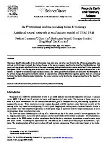
Figure 3 shows the NAR(1) time series of length n=200 with and without innovative outlier. The initial value on t=0 was x 0 = 0 , generated by the model (5.3). Figure 3 shows the NAR(1) time series of length n=200 with and without innovative outlier. The initial value on t=0 was x 0 = 0 , generated by the model (5.3).

X(t)

Time Series

3 2 1 0 -1 -2 -3 0

50

100

150

200

t NAR(1) without innovative outlier NAR(1) with innovative outlier

Fig. 3. NAR(1) Time series with and without innovative outliers.

To different FANN candidate architectures a quality factor defined by the local robustness is added. In this case some architectures are discovered to be better than others with respect to the local robustness measure studied as shown in Table 2 and Table 3 for the case of the time series without and with innovative outliers respectively.

Table 2. MSE: mean square error between the FANN and the noisy system outputs on the training set without innovative outliers and ∆ : distance between FANN output and the reference PDFs.

ANN

g NN 8

g NN 9

g NN10 g NN 11 g NN 12 g NN 13 g NN 14 g NN 15 g NN 16

MSE

0.1566 0.1502 0.1522 0.1605 0.1506 0.1594 0.1531 0.1501 0.1501

∆

0.1418 0.2274 0.1644 0.1581 0.2011 0.1634

0.202 0.3248 0.2666


171

Table 3. MSE: mean square error between the FANN and the noisy system outputs on the training set with innovative outliers and ∆ : distance between FANN output and the reference PDFs.

ANN

g NN 8

g NN 9

MSE 0.0954 0.0928

∆

g NN 10

g NN 11 g NN 12

0.086 0.0783 0.0795

g NN 13

g NN 14

g NN 15

g NN 16

0.061 0.0744 0.0563 0.0587

0.2239 0.118 0.2246 0.2324 0.2322 0.2283 0.2173 0.221

0.2944

It appears that the models g NN 8 and g NN 9 are the best FANN models for the NAR(1) without and with innovative outliers respectively in the sense of this quality factor. Figure 4 and Figure 5 shows the outputs PDFs of the different FANN architecture

6

Conclusions

A measure of local robustness has been applied to the problem of FANN architecture selection. The method is based in the comparison of the FANN output probability density function. For the output PDF comparison the Hellinger metric distance is used. However, it could be interesting to use a different distance measure. Only FANN architectures with one hidden layer have been considered. It has been shown that all FANN models are not necessarily equivalent in the sense of local robustness, around a particular sample. At present, there is little work on the analysis of the global or local robustness of FANN models with outliers in the input data space. For this reason further research is needed to study robustness properties in FANN with different architectures ( e.g., NAR(p); NARMA(p,q)) and other types of outliers (additive outliers and patchy outliers). Other future work in robust techniques and FANN will center around making neural networks robust to change in the variance noise. Nonlinear models are particularly sensitive to change in the variance. One would expect to see substantial improvements in FANN time series prediction if they can be robustified to the variance.

References [AlM 00] Allende H., Moraga C.: Time Series Forecasting with Neural Networks. Forschungsbericht N° 727/2000. Universität Dortmund Fachbereich Informatik. (2000)

172


Output Estimates PDFs of each FANN 6 5 4 3 2 1 0 -1,5

System Output PDF gnn8 output PDF gnn10 output PDF gnn11 output PDF gnn13 output PDF

-1

-0,5

0

X(t)

Fig. 4. Output estimates PDFs of the four most robust FANN for the NAR(1) time series without innovative outliers.

Output Estimates PDFs of each ANN

5 4

System Output PDF gnn8 output PDF

3

gnn9 output PDF gnn14 output PDF

2

gnn15 output PDF

1 0 -2,5

-2

X(t)

-1,5

-1

Fig. 5. Output estimates PDFs of the four most robust FANN for the NAR(1) time series with innovative outliers.

[AlH 92] Allende H., Heiler S.: Recursive Generalized M-Estimates for Autoregressive Moving Average Models. Journal of Time Series Analysis. 13, 1-18 (1992) [CaT 98] Castro J.L., Trillas E.: The logic of neural networks. Mathware and Softcomputing V (1), 23-27, (1998)


173

[ChC 99] Choueiki M.H. and Mount-Campbell C.A.: Training data development with the optimality criterion. IEEE Transactions on Neural Networks, 10, 56-63 (1999) [CoM 94] Connor J. T., Martin R. D.: Recurrent Neural Networks and Robust Time Series Prediction. IEEE Transactions of Neural Networks 5 (2), 240-253, (1994) [CoM 96] Connor J. T.: A robust Neural Networks Filter for Electricity Demand Prediction. J. of Forecasting 15, 437 – 458 (1996) [FaCh 98] Faraway J., Chatfield C.: Time series with Neural Networks. A comparative study using the airline data. Appl. Statist. 47 (2), 231 – 250 (1998) [Gab 98] Gabr M.M.: Robust estimation of bilinear time series models. Comm. Statist. Theory and Meth 27 (1), 41 – 53 (1998) [HaN 97] Hansen J., Nelson R.: Neural Networks and traditional time series methods. IEEE transaction on Neural Networks 8 (4), 863-873. (1997) [HeM 96] Heider R., Moraga C.; Evolutionary synthesis of neural networks based on graph-grammars. Proc. Int. Conf. On Soft and Intelligent Computing. 119-128, Budapest. ISBN 9634205100, (1996) [HiM 99] Hisham M. and Mount-Campell C.A. : Training data development with the D-optimality criterion. IEEE Transaction on Neural Networks Vol 10, 56-63 (1999) [LaF 95] Lachtermacher G. and Fuller J.D.: Backpropagation in Time Series. J. of Forecasting 14, 381-393 (1995) [MoS 01] Moraga C., Salinas L.: Interpreting neural networks in the frame of the logic of Lukasiewicz. Proceedings Int’l Workconference on artificial and natural neural networks IWANN’2001. Granada, Spain. Springer, (2001) [MoT 00] Moraga C., Temme K.-H.: S-neural networks are fuzzy models. Proceedings Int’l Conference on Information Processing and Management of Uncertainty in Knowledge based Systems, 1518-1523. Technical University of Madrid, Spain, (2000) [Sub 81] Subba Rao, T.: On the theory of bilinear time series models. Comm. Statist. Soc. B 43 (2), 244-255 (1981) [TKK 89] Tierney L., Kass R. and Kadane JB.: Approximative marginal densities of non-linear functions. Biometrika 76, 425-433. Correction in Biometrika 78, 233234. [Whi 89] White H.: Learning in Neural Networks: A statistical perspective. Neural Computation 1 425-464 (1989) [Whi 92] White H.: Artificial Neural Networks: Approximation and Learning Theory, Basil Blackwell, Oxford (1992) [Whi 94] White H.: Estimate Inference and Specification Analysis, New York: Cambridge University Press, (1994) [ReZ 99] Referes A. P. N., Zapranis A. D.: Neural Model Identification, Variable Selection and Model adequacy. J. Forecasting 18, 299-322, (1999). [Yao 99] Yao X.; Evolution of Artificial Neural Networks, Proc. IEEE 87 (9), 47-49. (1999)