Neural Models of Bayesian Belief Propagation Rajesh P. N. Rao

To appear in: The Bayesian Brain: Probabilistic Approaches to Neural Coding, K. Doya, S. Ishii, A. Pouget, R. P. N. Rao, eds., Cambridge, MA: MIT Press, 2006.

11 11.1

Neural Models of Bayesian Belief Propagation Rajesh P. N. Rao

Introduction Animals are constantly faced with the challenge of interpreting signals from noisy sensors and acting in the face of incomplete knowledge about the environment. A rigorous approach to handling uncertainty is to characterize and process information using probabilities. Having estimates of the probabilities of objects and events allows one to make intelligent decisions in the presence of uncertainty. A prey could decide whether to keep foraging or to flee based on the probability that an observed movement or sound was caused by a predator. Probabilistic estimates are also essential ingredients of more sophisticated decision-making routines such as those based on expected reward or utility. An important component of a probabilistic system is a method for reasoning based on combining prior knowledge about the world with current input data. Such methods are typically based on some form of Bayesian inference, involving the computation of the posterior probability distribution of one or more random variables of interest given input data. In this chapter, we describe how neural circuits could implement a general algorithm for Bayesian inference known as belief propagation. The belief propagation algorithm involves passing “messages” (probabilities) between the nodes of a graphical model that captures the causal structure of the environment. We review the basic notion of graphical models and illustrate the belief propagation algorithm with an example. We investigate potential neural implementations of the algorithm based on networks of leaky integrator neurons and describe how such networks can perform sequential and hierarchical Bayesian inference. Simulation results are presented for comparison with neurobiological data. We conclude the chapter by discussing other recent models of inference in neural circuits and suggest directions for future research. Some of the ideas reviewed in this chapter have appeared in prior publications [30, 31, 32, 42]; these may be consulted for additional details and results not included in this chapter.

236

11 Neural Models of Bayesian Belief Propagation

11.2

Rajesh P. N. Rao

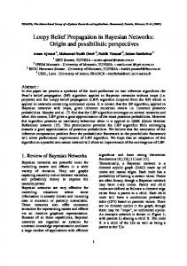
Bayesian Inference through Belief Propagation Consider the problem of an animal deciding whether to flee or keep feeding based on the cry of another animal from a different species. Suppose it is often the case that the other animal emits the cry whenever there is a predator in the vicinity. However, the animal sometimes also emits the same cry when a potential mate is in the area. The probabilistic relationship between a cry and its probable causes can be captured using a graphical model as shown in figure 11.1. The circles (or nodes) represent the two causes and the observation as random variables R (Predator), M (Mate), and C (Cry heard). We assume these random variables are binary and can take on the values 1 and 0 (for “presence” and “absence” respectively), although this can be generalized to multiple values. The arcs connecting the nodes represent the probabilistic causal relationships as characterized by the probability table P (C|R, M ).

Predator (R)

Mate (M)

Cry Heard (C) Figure 11.1 An Example of a Graphical Model. Each circle represents a node denoting a random variable. Arrows represent probabilistic dependencies as specified by the probability table P (C|R, M ).

For the above problem, the decision to flee or not can be based on the posterior probability P (R|C) of a predator given that a cry was heard (C = 1). This probability can be calculated directly as: X P (R = 1|C = 1) = P (R = 1, M |C = 1) M

=

X

kP (C = 1|R = 1, M )P (R = 1)P (M ),

(11.1)

M

where we used Bayes rule to obtain P the second equation from the first, with k being the normalization constant 1/ R,M P (C = 1|R, M )P (R)P (M ). The above calculation required summing over the random variable M that was irrelevant to the problem at hand. In a general scenario, one would need to sum over all irrelevant random variables, an operation which scales exponentially with the total number of variables, quickly becoming intractable. Fortunately, there exists an alternate method known as belief propagation (or prob-

11.2

Bayesian Inference through Belief Propagation

237

ability propagation) [26] that involves passing messages (probability vectors) between the nodes of the graphical model and summing over local products of messages, an operation that can be tractable. The belief propagation algorithm involves two types of computation: marginalization (summation over local joint distributions) and multiplication of local marginal probabilities. Because the operations are local, the algorithm is also well suited to neural implementation, as we shall discuss below. The algorithm is provably correct for singly connected graphs (i.e., no undirected cycles) [26], although it has been used with some success in some graphical models with cycles as well [25].

11.2.1

A Simple Example We illustrate the belief propagation algorithm using the feed-or-flee problem above. The nodes R and M first generate the messages P (R) and P (M ) respectively, which are vectors of length two storing the prior probabilities for R = 0 and 1, and M = 0 and 1 respectively. These messages are sent to node C. Since a cry was heard, the value of C is known (C = 1) and therefore, the messages from R and M do not affect node C. We are interested in computing the marginal probabilities for the two hidden nodes R and M . The node C generates the message mC→R = mC→M = (0, 1), i.e., probability of absence of a cry is 0 and probability of presence of a cry is 1 (since a cry was heard). This message is passed on to the nodes R and M . Each node performs a marginalization over variables other than itself using the local conditional probability table P and the incoming messages.PFor example, in the case of node R, this is M,C P (C|R, M )P (M )P (C) = M P (C = 1|R, M )P (M ) since P C is known to be 1. Similarly, P the node M performs the marginalization R,C P (C|R, M )P (R)P (C) = R P (C = 1|R, M )P (R). The final step involves multiplying these marginalized probabilities with other messages received, in this case, P (R) and P (M ) respectively, to yield, after normalization, the posterior probability of R and M given the observation C = 1: ³X ´ P (R|C = 1) = α P (C = 1|R, M )P (M ) P (R) (11.2) M

P (M |C = 1) =

β

³X

´ P (C = 1|R, M )P (R) P (M ),

(11.3)

R

where α and β are normalization constants. Note that equation (11.2) above yields the same expression for P (R = 1|C = 1) as equation (11.1) that was derived using Bayes rule. In general, belief propagation allows efficient computation of the posterior probabilities of unknown random variables in singly connected graphical models, given any available evidence in the form of observed values for any subset of the random variables.

11.2.2

Belief Propagation over Time Belief propagation can also be applied to graphical models evolving over time. A simple but widely used model is the hidden Markov model (HMM) shown

238


Rajesh P. N. Rao

in figure 11.2A. The input that is observed at time t (= 1, 2, . . .) is represented by the random variable I(t), which can either be discrete-valued or a real-valued vector such as an image or a speech signal. The input is assumed to be generated by a hidden cause or “state” θ(t), which can assume one of N discrete values 1, . . . , N . The state θ(t) evolves over time in a Markovian manner, depending only on the previous state according to the transition probabilities given by P (θ(t) = i|θ(t − 1) = j) = P (θit |θjt−1 ) for i, j = 1 . . . N . The observation I(t) is generated according to the probability P (I(t)|θ(t)). The belief propagation algorithm can be used to compute the posterior probability of the state given current and past inputs (we consider here only the “forward” propagation case, corresponding to on-line state estimation). As in the previous example, the node θt performs a marginalization over neighboring variables, in this case θt−1 and I(t). The first marginalization results in a P probability vector whose ith component is j P (θit |θjt−1 )mjt−1,t where mjt−1,t is t−1 the jth component of the message from node to θt . The second marginalP θ ization is from node I(t) and is given by I(t) P (I(t)|θit )P (I(t)). If a particuP lar input I0 is observed, this sum becomes I(t) P (I(t)|θit )δ(I(t), I0 ) = P (I0 |θit ), where δ is the delta function which evaluates to 1 if its two arguments are equal and 0 otherwise. The two “messages” resulting from the marginalization along the arcs from θt−1 and I(t) can be multiplied at node θt to yield the following message to θt+1 : X mt,t+1 = P (I0 |θit ) P (θit |θjt−1 )mt−1,t (11.4) i j j

If m0,1 = P (θi ) (the prior distribution over states), then it is easy to show using i Bayes rule that mt,t+1 = P (θit , I(t), . . . , I(1)). i Rather than computing the joint probability, one is typically interested in calculating the posterior probability of the state, given current and past inputs, i.e., P (θit |I(t), . . . , I(1)). This can be done by incorporating a normalization step at each time step. Define (for t = 1, 2, . . .): X mti = P (I0 |θit ) P (θit |θjt−1 )mt−1,t (11.5) j j

mt,t+1 i

mti /nt ,

= (11.6) P where nt = j mtj . If m0,1 = P (θi ) (the prior distribution over states), then it i is easy to see that: mt,t+1 = P (θit |I(t), . . . , I(1)) i

(11.7)

This method has the additional advantage that the normalization at each time step promotes stability, an important consideration for recurrent neuronal networks, and allows the likelihood function P (I0 |θit ) to be defined in proportional terms without the need for explicitly calculating its normalization factor (see section 11.4 for an example).

11.2

239

Bayesian Inference through Belief Propagation

t θt

t+1

θ t+1

I(t+1)

I(t)

B

A

I(t)

Figure 11.2 Graphical Model for a HMM and its Neural Implementation. (A) Dynamic graphical model for a hidden Markov model (HMM). Each circle represents a node denoting the state variable θt which can take on values 1, . . . , N . (B) Recurrent network for implementing on-line belief propagation for the graphical model in (A). Each circle represents a neuron encoding a state i. Arrows represent synaptic connections. The probability distribution over state values at each time step is represented by the entire population. A

B Locations (L)

Features (F)

Location Coding Neurons

Feature Coding Neurons

Intermediate Representation (C) Image (I)

Image

Figure 11.3 A Hierarchical Graphical Model for Images and its Neural Implementation. (A) Three-level graphical model for generating simple images containing one of many possible features at a particular location. (B) Three-level network for implementing on-line belief propagation for the graphical model in (A). Arrows represent synaptic connections in the direction pointed by the arrow heads. Lines without arrow heads represent bidirectional connections.

11.2.3

Hierarchical Belief Propagation As a third example of belief propagation, consider the three-level graphical model shown in figure 11.3A. The model describes a simple process for generating images based on two random variables: L, denoting spatial locations, and F , denoting visual features (a more realistic model would involve a hierarchy of such features, sub-features, and locations). Both random variables are assumed to be discrete, with L assuming one of n values L1 , . . . , Ln , and F assuming one of m different values F1 , . . . , Fm . The node C denotes different combinations of features and locations, each of its values C1 , . . . , Cp encoding a specific feature at a specific location. Representing all possible combinations is infeasible but it is sufficient to represent those that occur frequently and to map

240


Rajesh P. N. Rao

each feature-location (L, F ) combination to the closest Ci using an appropriate distribution P (Ci |L, F ) (see section 11.4 for an example). An image with a specific feature at a specific location is generated according to the image likelihood P (I|C). Given the above graphical model for images, we are interested in computing the posterior probabilities of features (more generally, objects or object parts) and their locations in an input image. This can be done using belief propagation. Given the model in figure 11.3A and a specific input image I = I 0 , belief propagation prescribes that the following ?messages? (probabilities) be transmitted from one node to another, as given by the arrows in the subscripts: mL→C mF →C mI→C mC→L

= P (L) = P (F ) = P (I = I 0 |C) XX = P (C|L, F )P (F )P (I = I 0 |C) F

mC→F

=

(11.11)

C

XX L

(11.8) (11.9) (11.10)

P (C|L, F )P (L)P (I = I 0 |C)

(11.12)

C

The first three messages above are simply prior probabilities encoding beliefs about locations and features before a sensory input becomes available. The posterior probabilities of the unknown variables C, L, and F given the input image I, are calculated by combining the messages at each node as follows: XX P (C|I = I 0 ) = αmI→C P (C|L, F )mL→C mF →C (11.13) F

P (L|I = I 0 ) P (F |I = I 0 )

L

= βmC→L P (L) = γmC→F P (F ),

(11.14) (11.15)

where α, β, and γ are normalization constants that make each of the above probabilities sum to 1. Note how the prior P (L) multiplicatively modulates the posterior probability of a feature in equation 11.15 via equation 11.12. This observation plays an important role in section 11.4 below where we simulate spatial attention by increasing P (L) for a desired location.

11.3 11.3.1

Neural Implementations of Belief Propagation Approximate Inference in Linear Recurrent Networks We begin by considering a commonly used neural architecture for modeling cortical response properties, namely, a linear recurrent network with firingrate dynamics (see, for example, [5]). Let I denote the vector of input firing rates to the network and let v represent the output firing rates of N recurrently connected neurons in the network. Let W represent the feedforward synaptic weight matrix and M the recurrent weight matrix. The following equation

11.3

241

Neural Implementations of Belief Propagation

describes the dynamics of the network: τ

dv = −v + WI + Uv, dt

(11.16)

where τ is a time constant. The equation can be written in a discrete form as follows: X vi (t + 1) = vi (t) + ²(−vi (t) + wi I(t) + uij vj (t)), (11.17) j

where ² is the integration rate, vi is the ith component of the vector v, wi is the ith row of the matrix W, and uij is the element of U in the ith row and jth column. The above equation can be rewritten as: X vi (t + 1) = ²wi I(t) + Uij vj (t), (11.18) j

where Uij = ²uij for i 6= j and Uii = 1 + ²(uii − 1). Comparing the belief propagation equation (11.5) for a HMM with equation (11.18) above, it can be seen that both involve propagation of quantities over time with contributions from the input and activity from the previous time step. However, the belief propagation equation involves multiplication of these contributions while the leaky integrator equation above involves addition. Now consider belief propagation in the log domain. Taking the logarithm of both sides of equation (11.5), we get: X log mti = log P (I0 |θit ) + log P (θit |θjt−1 )mjt−1,t (11.19) j

This equation is much more conducive to neural implementation via equation (11.18). In particular, equation (11.18) can implement equation (11.19) if: vi (t + 1) = log mti ²wi I(t) = log P (I0 |θit ) X X Uij vj (t) = log P (θit |θjt−1 )mt−1,t j j

(11.20) (11.21) (11.22)

j

The normalization step (equation (11.6)) can be computed by a separate group t,t+1 of neurons representing mP that receive as excitatory input log mti and ini t hibitory input log n = log j mtj : log mt,t+1 i

=

log mti − log nt

(11.23)

These neurons convey the normalized posterior probabilities mt,t+1 back to i the neurons implementing equation (11.19) so that mt+1 may be computed at i the next time step. Note the the normalization step makes the overall network nonlinear. In equation (11.21), the log-likelihood log P (I0 |θit ) is calculated using a linear operation ²wi I(t) (see also [45]). Since the messages are normalized at each

242


Rajesh P. N. Rao

time step, one can relax the equality in equation (11.21) and make log P (I0 |θit ) ∝ F(θi )I(t) for some linear filter F(θi ) = ²wi . This avoids the problem of calculating the normalization factor for P (I0 |θit ), which can be especially hard when I0 takes on continuous values such as in an image. A more challenging problem is to pick recurrent weights Uij such that equation (11.22) holds true. For equation (11.22) to hold true, we need to approximate a log-sum with a sum-of-logs. One approach is to generate a set of random probabilities xj (t) for t = 1, . . . , T and find a set of weights Uij that satisfy: X

Uij log xj (t) ≈ log

·X

j

¸ P (θit |θjt−1 )xj (t)

(11.24)

j

for all i and t. This can be done by minimizing the squared error in equation (11.24) with respect to the recurrent weights Uij . This empirical approach, followed in [30], is used in some of the experiments below. An alternative approach is to exploit the nonlinear properties of dendrites as suggested in the following section.

11.3.2

Exact Inference in Nonlinear Networks A firing rate model that takes into account some of the effects of nonlinear filtering in dendrites can be obtained by generalizing equation (11.18) as follows: ¡ ¢ ¡X ¢ vi (t + 1) = f wi I(t) + g Uij vj (t) ,

(11.25)

j

where f and g model nonlinear dendritic filtering functions for feedforward and recurrent inputs. By comparing this equation with the belief propagation equation in the log domain (equation (11.19)), it can be seen that the first equation can implement the second if: vi (t + 1) = log mti ¡ ¢ f wi I(t) = log P (I0 |θit ) X ¡X ¢ g Uij vj (t) = log P (θit |θjt−1 )mjt−1,t j

(11.26) (11.27) (11.28)

j

In this model (figure 11.2B), N neurons represent log mti (i = 1, . . . , N ) in their firing rates. The dendritic filtering functions f and g approximate the logarithm function, the feedforward weights wi act as a linear filter on the input to yield the likelihood P (I0 |θit ) and the recurrent synaptic weights Uij directly encode the transition probabilities P (θit |θjt−1 ). The normalization step is computed as in equation (11.23) using a separate group of neurons that represent log posterior probabilities log mt,t+1 and that convey these probabilities for use i in equation (11.28) by the neurons computing log mt+1 . i

11.3

11.3.3

243

Neural Implementations of Belief Propagation

Inference Using Noisy Spiking Neurons Spiking Neuron Model The models above were based on firing rates of neurons, but a slight modification allows an interpretation in terms of noisy spiking neurons. Consider a variant of equation (11.16) where v represents the membrane potential values of neurons rather than their firing rates. We then obtain the classic equation describing the dynamics of the membrane potential vi of neuron i in a recurrent network of leaky integrate-and-fire neurons: X X dvi τ = −vi + wij Ij + uij vj0 , (11.29) dt j j where τ is the membrane time constant, Ij denotes the synaptic current due to input neuron j, wij represents the strength of the synapse from input j to recurrent neuron i, vj0 denotes the synaptic current due to recurrent neuron j, and uij represents the corresponding synaptic strength. If vi crosses a threshold T , the neuron fires a spike and vi is reset to the potential vreset . Equation (11.29) can be rewritten in discrete form as: X X vi (t + 1) = vi (t) + ²(−vi (t) + wij Ij (t)) + uij vj0 (t)) (11.30) i.e.

vi (t + 1)

= ²

X

wij Ij (t) +

j

X

j

Uij vj0 (t),

j

(11.31)

j

where ² is the integration rate, Uii = 1 + ²(uii − 1) and for i 6= j, Uij = ²uij . The nonlinear variant of the above equation that includes dendritic filtering of input currents in the dynamics of the membrane potential is given by: ¡X ¢ ¡X ¢ vi (t + 1) = f wij Ij (t) + g Uij vj0 (t) , (11.32) j

j

where f and g are nonlinear dendritic filtering functions for feedforward and recurrent inputs. We can model the effects of background inputs and the random openings of membrane channels by adding a Gaussian white noise term to the right-hand side of equations (11.31) and (11.32). This makes the spiking of neurons in the recurrent network stochastic. Plesser and Gerstner [27] and Gerstner [11] have shown that under reasonable assumptions, the probability of spiking in such noisy neurons can be approximated by an “escape function” (or hazard function) that depends only on the distance between the (noise-free) membrane potential vi and the threshold T . Several different escape functions were found to yield similar results. We use the following exponential function suggested in [11] for noisy integrate-and-fire networks: P (neuron i spikes at time t) = ke(vi (t)−T ) ,

(11.33)

where k is an arbitrary constant. We use a model that combines equations (11.32) and (11.33) to generate spikes.

244


Rajesh P. N. Rao

Inference in Spiking Networks By comparing the membrane potential equation (11.32) with the belief propagation equation in the log domain (equation (11.19)), we can postulate the following correspondences:

f

¡X j

g

¡X

vi (t + 1) = log mti ¢ wij Ij (t) = log P (I0 |θit ) ¢ Uij vj0 (t)

j

=

log

X

(11.34) (11.35)

P (θit |θjt−1 )mt−1,t j

(11.36)

j

The dendritic filtering functions f and g approximate the logarithm function, the synaptic currents Ij (t) and vj0 (t) are approximated by the corresponding instantaneous firing rates, and the recurrent synaptic weights Uij encode the transition probabilities P (θit |θjt−1 ). Since the membrane potential vi (t+1) is assumed to be equal to log mti (equation (11.34)), we can use equation (11.33) to calculate the probability of spiking for each neuron i as: P (neuron i spikes at time t + 1) ∝ e(vi (t+1)−T ) (log mti −T )

∝ e ∝ mti

(11.37) (11.38) (11.39)

Thus, the probability of spiking (or, equivalently, the instantaneous firing rate) for neuron i in the recurrent network is directly proportional to the message mti , which is the posterior probability of the neuron’s preferred state and current input given past inputs. Similarly, the instantaneous firing rates of the group of neurons representing log mt,t+1 is proportional to mt,t+1 , which is the precisely i i the input required by equation (11.36).

11.4 11.4.1

Results Example 1: Detecting Visual Motion We first illustrate the application of the linear firing rate-based model (section 11.3.1) to the problem of detecting visual motion. A prominent property of visual cortical cells in areas such as V1 and MT is selectivity to the direction of visual motion. We show how the activity of such cells can be interpreted as representing the posterior probability of stimulus motion in a particular direction, given a series of input images. For simplicity, we focus on the case of 1D motion in an image consisting of X pixels with two possible motion directions: leftward (L) or rightward (R). Let the state θij represent a motion direction j ∈ {L, R} at spatial location i. Consider a network of N neurons, each representing a particular state θij (figure 11.4A). The feedforward weights are assumed to be Gaussians, i.e. F(θiR ) = F(θiL ) = F(θi ) = Gaussian centered at location i with a standard

11.4

245

Results

deviation σ. Figure 11.4B depicts the feedforward weights for a network of 30 neurons, 15 encoding leftward and 15 encoding rightward motion. F ( θ 15 )

F ( θ 1)

P( θ iR | θ kR )

0.30.3

P( θ iL | θ jL )

Rightward

0.2 0.2

Leftward 0.10.1

F ( θ i) Image

00

0

5

1

10 10

15

20 20

25

30 30

Spatial Location (pixels)

B

A θ t−1 1

From Neuron j

15

30

1

5

5

10

10

To Neuron i

θt

15

30

1

1

1515 20

20 25

25

3030

1515

Rightward 5

10

Leftward 15

C

20

25

30

3030

Rightward 5

10

Leftward 15

D

20

25

30

Figure 11.4 Recurrent Network for Motion Detection (from [30]). (A) depicts a recurrent network of neurons, shown for clarity as two chains selective for leftward and rightward motion respectively. The feedforward synaptic weights for neuron i (in the leftward or rightward chain) are determined by F(θi ). The recurrent weights reflect the transition probabilities P (θiR |θkR ) and P (θiL |θjL ). (B) Feedforward weights F(θi ) for neurons i = 1, . . . , 15 (rightward chain). The feedforward weights for neurons i = 15, . . . , 30 (leftward chain) are identical. (C) Transition probabilities P (θt |θt−1 ). Probability values are proportional to pixel brightness. (D) Recurrent weights Uij computed from the transition probabilities in (C) using Equation 11.24.

We model visual motion using an HMM. The transition probabilities P (θij |θkl ) are selected to reflect both the direction of motion and speed of the moving stimulus. The transition probabilities for rightward motion from the state θkR (i.e. P (θiR |θkR )) were set according to a Gaussian centered at location k + x, where x is a parameter determined by stimulus speed. The transition probabilities for leftward motion from the state θkL were likewise set to Gaussian values centered at k − x. The transition probabilities from states near the two boundaries (i = 1 and i = X) were chosen to be uniformly random values. Figure 11.4C shows the matrix of transition probabilities.

246


Rajesh P. N. Rao

Recurrent Network Model To detect motion using Bayesian inference in the above HMM, consider first a model based on the linear recurrent network as in equation (11.18) but with normalization as in equation (11.23) (which makes the network nonlinear). We can compute the recurrent weights mij for the transition probabilities given above using the approximation method in equation (11.24) (see figure 11.4D). The resulting network then implements approximate belief propagation for the HMM based on equation (11.20-11.23). Figure 11.5 shows the output of the network in the middle of a sequence of input images depicting a bar moving either leftward or rightward. As shown in the figure, for a leftward-moving bar at a particular location i, the highest network output is for the neuron representing location i and direction L, while for a rightward-moving bar, the neuron representing location i and direction R has the highest output. The output firing rates were computed from the log probabilities log mt,t+1 using a simple linear i encoding model: fi = [c · vi + F ]+ where c is a positive constant (= 12 for this plot), F is the maximum firing rate of the neuron (= 100 in this example), and + denotes rectification. Note that even though the log-likelihoods are the same for leftward- and rightward-moving inputs, the asymmetric recurrent weights (which represent the transition probabilities) allow the network to distinguish between leftward- and rightward-moving stimuli. The posterior probabilities mt,t+1 are shown in figure 11.5 (lowest panels). The network correctly comi putes posterior probabilities close to 1 for the states θiL and θiR for leftward and rightward motion respectively at location i.

00

Rightward Moving Input

00

5

10

5

10

−5

−10 −10 −15

100 100 5050 00 11 0.50.5 00 1

15

20

25

30

15

20

25

30

log posterior

firing rate 5

10

15

20

5

10

15 15

20

0 −5 −10 −15 100

5

10

15

20

25

30

5

10

15

20

25

30

5

10

15

20

25

30

5

10

15 15

20

25

30 30

50 25

30

posterior

Right selective neurons

Leftward Moving Input

0 −1 −2

log likelihood

−1 −2−2

0 1 0.5

25

30 30

Left selective neurons

0

1

Right selective neurons

Left selective neurons

Figure 11.5 Network Output for a Moving Stimulus (from [30]). (Left Panel) The four plots depict respectively the log likelihoods, log posteriors, neural firing rates, and posterior probabilities observed in the network for a rightward moving bar when it arrives at the central image location. Note that the log likelihoods are the same for the rightward and leftward selective neurons (the first 15 and last 15 neurons respectively, as dictated by the feedforward weights in Figure 11.4B) but the outputs of these neurons correctly reflect the direction of motion as a result of recurrent interactions. (Right Panel) The same four plots for a leftward moving bar as it reaches the central location.

11.4

247

Results

Nonlinear Spiking Model The motion detection task can also be solved using a nonlinear network with spiking neurons as described in section 11.3.3. A single-level recurrent network of 30 neurons as in the previous section was used. The feedforward weights were the same as in figure 11.4B. The recurrent connections directly encoded transition probabilities for leftward motion (see figure 11.4C). As seen in figure 11.6A, neurons in the network exhibited direction selectivity. Furthermore, the spiking probability of neurons reflects the probability mti of motion direction at a given location as in equation (11.39) (figure 11.6B), suggesting a probabilistic interpretation of direction-selective spiking responses in visual cortical areas such as V1 and MT. Rightward Motion

Leftward Motion

Neuron

8 10 12

A Neuron

8

0.5

0.5

0.4

0.4

0.3

0.2

0.1

0

10

0.3

0.2

0.1

5

10

15

20

0.5

0.5

0.4

0.4

0.3

0

10

15

20

25

30

5

10

15

20

25

30

5

10

15

20

25

30

0.2

0.1

5

10

15

20

0

25

0.5

0.5

0.4

0.4

0.3

0.3

0.2

0.2

0.1

0

5

0.3

0.2

0.1

12

0

25

0.1

5

10

15

20

0

25

B Figure 11.6 Responses from the Spiking Motion Detection Network. (A) Spiking responses of three of the first 15 neurons in the recurrent network (neurons 8, 10, and 12). As is evident, these neurons have become selective for rightward motion as a consequence of the recurrent connections (= transition probabilities) specified in Figure 11.4C. (B) Posterior probabilities over time of motion direction (at a given location) encoded by the three neurons for rightward and leftward motion.

11.4.2

Example 2: Bayesian Decision-Making in a Random-Dots Task To establish a connection to behavioral data, we consider the well-known random dots motion discrimination task (see, for example, [41]). The stimulus consists of an image sequence showing a group of moving dots, a fixed fraction of which are randomly selected at each frame and moved in a fixed direction (for example, either left or right). The rest of the dots are moved in

248


Rajesh P. N. Rao

random directions. The fraction of dots moving in the same direction is called the coherence of the stimulus. Figure 11.7A depicts the stimulus for two different levels of coherence. The task is to decide the direction of motion of the coherently moving dots for a given input sequence. A wealth of data exists on the psychophysical performance of humans and monkeys as well as the neural responses in brain areas such as the middle temporal (MT) and lateral intraparietal areas (LIP) in monkeys performing the task (see [41] and references therein). Our goal is to explore the extent to which the proposed models for neural belief propagation can explain the existing data for this task. The nonlinear motion detection network in the previous section computes the posterior probabilities P (θiL |I(t), . . . , I(1)) and P (θiR |I(t), . . . , I(1)) of leftward and rightward motion at different locations i. These outputs can be used to decide the direction of coherent motion by computing the posterior probabilities for leftward and rightward motion irrespective of location, given the input images. These probabilities can be computed by marginalizing the posterior distribution computed by the neurons for leftward (L) and rightward (R) motion over all spatial positions i: X P (L|I(t), . . . , I(1)) = P (θiL |I(t), . . . , I(1)) (11.40) i

P (R|I(t), . . . , I(1)) =

X

P (θiR |I(t), . . . , I(1))

(11.41)

i

To decide the overall direction of motion in a random-dots stimulus, there exist two options: (1) view the decision process as a “race” between the two probabilities above to a prechosen threshold (this also generalizes to more than two choices); or (2) compute the log of the ratio between the two probabilities above and compare this log-posterior ratio to a prechosen threshold. We use the latter method to allow comparison to the results of Shadlen and colleagues, who postulate a ratio-based model in area LIP in primate parietal cortex [12]. The log-posterior ratio r(t) of leftward over rightward motion can be defined as: r(t)

= =

log P (L|I(t), . . . , I(1)) − log P (R|I(t), . . . , I(1)) P (L|I(t), . . . , I(1)) log P (R|I(t), . . . , I(1))

(11.42) (11.43)

If r(t) > 0, the evidence seen so far favors leftward motion and vice versa for r(t) < 0. The instantaneous ratio r(t) is susceptible to rapid fluctuations due to the noisy stimulus. We therefore use the following decision variable dL (t) to track the running average of the log posterior ratio of L over R: dL (t + 1)

= dL (t) + α(r(t) − dL (t))

(11.44)

and likewise for dR (t) (the parameter α is between 0 and 1). We assume that the decision variables are computed by a separate set of “decision neurons” that receive inputs from the motion detection network. These neurons are once

11.4

Results

249

again leaky-integrator neurons as described by Equation 11.44, with the driving inputs r(t) being determined by inhibition between the summed inputs from the two chains in the motion detection network (as in equation (11.42)). The output of the model is “L” if dL (t) > c and “R” if dR (t) > c, where c is a “confidence threshold” that depends on task constraints (for example, accuracy vs. speed requirements) [35]. Figure 11.7B and C shows the responses of the two decision neurons over time for two different directions of motion and two levels of coherence. Besides correctly computing the direction of coherent motion in each case, the model also responds faster when the stimulus has higher coherence. This phenomenon can be appreciated more clearly in figure 11.7D, which predicts progressively shorter reaction times for increasingly coherent stimuli (dotted arrows). Comparison to Neurophysiological Data The relationship between faster rates of evidence accumulation and shorter reaction times has received experimental support from a number of studies. Figure 11.7E shows the activity of a neuron in the frontal eye fields (FEF) for fast, medium, and slow responses to a visual target [39, 40]. Schall and collaborators have shown that the distribution of monkey response times can be reproduced using the time taken by neural activity in FEF to reach a fixed threshold [15]. A similar rise-to-threshold model by Carpenter and colleagues has received strong support in human psychophysical experiments that manipulate the prior probabilities of targets [3] and the urgency of the task [35]. In the case of the random-dots task, Shadlen and collaborators have shown that in primates, one of the cortical areas involved in making the decision regarding coherent motion direction is area LIP. The activities of many neurons in this area progressively increase during the motion-viewing period, with faster rates of rise for more coherent stimuli (see figure 11.7F) [37]. This behavior is similar to the responses of “decision neurons” in the model (figure 11.7B–D), suggesting that the outputs of the recorded LIP neurons could be interpreted as representing the log-posterior ratio of one task alternative over another (see [3, 12] for related suggestions).

11.4.3

Example 3: Attention in the Visual Cortex The responses of neurons in cortical areas V2 and V4 can be significantly modulated by attention to particular locations within an input image. McAdams and Maunsell [23] showed that the tuning curve of a neuron in cortical area V4 is multiplied by an approximately constant factor when the monkey focuses attention on a stimulus within the neuron’s receptive field. Reynolds et al. [36] have shown that focusing attention on a target in the presence of distractors causes the response of a V2 or V4 neuron to closely approximate the response elicited when the target appears alone. Finally, a study by Connor et al. [4] demonstrated that responses to unattended stimuli can be affected by spatial

250


Rajesh P. N. Rao

attention to nearby locations. All three types of response modulation described above can be explained in terms of Bayesian inference using the hierarchical graphical model for images given in section 11.2.3 (figure 11.3). Each V4 neuron is assumed to encode a feature Fi as its preferred stimulus. A separate group of neurons (e.g., in the parietal cortex) is assumed to encode spatial locations (and potentially other spatiotemporal transformations) irrespective of feature values. Lower-level neurons (for example, in V2 and V1) are assumed to represent the intermediate representations Ci . Figure 11.3B depicts the corresponding network for neural belief propagation. Note that this network architecture mimics the division of labor between the ventral object processing ("what") stream and the dorsal spatial processing ("where") stream in the visual cortex [24]. The initial firing rates of location- and feature-coding neurons represent prior probabilities P (L) and P (F ) respectively, assumed to be set by taskdependent feedback from higher areasP such as those in prefrontal cortex. The input likelihood P (I = I 0 |C) is set to j wij Ij , where the weights wij represent the attributes of Ci (specific feature at a specific location). Here, we set these weights to spatially localized oriented Gabor filters. equation (11.11) and (11.12) are assumed to be computed by feedforward neurons in the locationcoding and feature-coding parts of the network, with their synapses encoding P (C|L, F ). Taking the logarithm of both sides of equations (11.13-11.15), we obtain equations that can be computed using leaky integrator neurons as in equation (11.32) (f and g are assumed to approximate a logarithmic transformation). Recurrent connections in equation (11.32) are used to implement the inhibitory component corresponding to the negative logarithm of the normalization constants. Furthermore, since the membrane potential vi (t) is now equal to the log of the posterior probability, i.e., vi (t) = log P (F |I = I 0 ) (and similarly for L and C), we obtain, using equation (11.33): P (feature coding neuron i spikes at time t) ∝ P (F |I = I 0 )

(11.45)

This provides a new interpretation of the spiking probability (or instantaneous firing rate) of a V4 neuron as representing the posterior probability of a preferred feature in an image (irrespective of spatial location). To model the three primate experiments discussed above [4, 23, 36], we used horizontal and vertical bars that could appear at nine different locations in the input image (figure 11.8A). All results were obtained using a network with a single set of parameters. P (C|L, F ) was chosen such that for any given value of L and F , say location Lj and feature Fk , the value of C closest to the combination (Lj , Fk ) received the highest probability, with decreasing probabilities for neighboring locations (see figure 11.8B). Multiplicative Modulation of Responses We simulated the attentional task of McAdams and Maunsell [23] by presenting a vertical bar and a horizontal bar simultaneously in an input image. “Attention” to a location Li containing one of the bars was simulated by setting

11.4

Results

251

a high value for P (Li ), corresponding to a higher firing rate for the neuron coding for that location. Figure 11.9A depicts the orientation tuning curves of the vertical feature coding model V4 neuron in the presence and absence of attention (squares and circles respectively). The plotted points represent the neuron’s firing rate, encoding the posterior probability P (F |I = I 0 ), F being the vertical feature. Attention in the model approximately multiplies the “unattended” responses by a constant factor, similar to V4 neurons (figure 11.9B). This is due to the change in the prior P (L) between the two modes, which affects equation (11.12) and (11.15) multiplicatively. Effects of Attention on Responses in the Presence of Distractors To simulate the experiments of Reynolds et al. [36], a single vertical bar (“Reference”) were presented in the input image and the responses of the vertical feature coding model neuron were recorded over time. As seen in figure 11.10A (top panel, dotted line), the neuron’s firing rate reflects a posterior probability close to 1 for the vertical stimulus. When a horizontal bar (“Probe”) alone is presented at a different location, the neuron’s response drops dramatically (solid line) since its preferred stimulus is a vertical bar, not a horizontal bar. When the horizontal and vertical bars are simultaneously presented (“Pair”), the firing rate drops to almost half the value elicited for the vertical bar alone (dashed line), signaling increased uncertainty about the stimulus compared to the Reference-only case. However, when “attention” is turned on by increasing P (L) for the vertical bar location (figure 11.10A, bottom panel), the firing rate is restored back to its original value and a posterior probability close to 1 is signaled (topmost plot, dot-dashed line). Thus, attention acts to reduce uncertainty about the stimulus given a location of interest. Such behavior closely mimics the effect of spatial attention in areas V2 and V4 [36] (figure 11.10B). Effects of Attention on Neighboring Spatial Locations We simulated the experiments of Connor et al. [4] using an input image containing four fixed horizontal bars as shown in figure 11.11A. A vertical bar was flashed at one of five different locations in the center (figure 11.11A, 1-5). Each bar plot in figure 11.11B shows the responses of the vertical feature coding model V4 neuron as a function of vertical bar location (bar positions 1 through 5) when attention is focused on one of the horizontal bars (left, right, upper, or lower). Attention was again simulated by assigning a high prior probability for the location of interest. As seen in figure 11.11B, there is a pronounced effect of proximity to the locus of attention: the unattended stimulus (vertical bar) produces higher responses when it is closer to the attended location than further away (see, for example, “Attend Left”). This effect is due to the spatial spread in the conditional probability P (C|L, F ) (see figure 11.8B), and its effect on equation (11.12) and (11.15). The larger responses near the attended location reflect a reduction

252


Rajesh P. N. Rao

in uncertainty at locations closer to the focus of attention compared to locations farther away. For comparison, the responses from a V4 neuron are shown in figure 11.11C (from [4]).

11.5

Discussion This chapter described models for neurally implementing the belief propagation algorithm for Bayesian inference in arbitrary graphical models. Linear and nonlinear models based on firing rate dynamics, as well as a model based on noisy spiking neurons, were presented. We illustrated the suggested approach in two domains: (1) inference over time using an HMM and its application to visual motion detection and decision-making, and (2) inference in a hierarchical graphical model and its application to understanding attentional effects in the primate visual cortex. The approach suggests an interpretation of cortical neurons as computing the posterior probability of their preferred state, given current and past inputs. In particular, the spiking probability (or instantaneous firing rate) of a neuron can be shown to be directly proportional to the posterior probability of the preferred state. The model also ascribes a functional role to local recurrent connections (lateral/horizontal connections) in the neocortex: connections from excitatory neurons are assumed to encode transition probabilities between states from one time step to the next, while inhibitory connections are used for probability normalization (see equation (11.23)). Similarly, feedback connections from higher to lower areas are assumed to convey prior probabilities reflecting prior knowledge or task constraints, as used in the attention model in section 11.4.3.

11.5.1

Related Models A number of models have been proposed for probabilistic computation in networks of neuron-like elements. These range from early models based on statistical mechanics (such as the Boltzmann machine [19, 20]) to more recent models that explicitly rely on probabilistic generative or causal models [6, 10, 29, 33, 43, 44, 45]. We review in more detail some of the models that are closely related to the approach presented in this chapter. Models based on Log-Likelihood Ratios Gold and Shadlen [12] have proposed a model for neurons in area LIP that interprets their responses as representing the log-likelihood ratio between two alternatives. Their model is inspired by neurophysiological results from Shadlen’s group and others showing that the responses of neurons in area LIP exhibit a behavior similar to a random walk to a fixed threshold. The neuron’s response increases given evidence in favor of the neuron’s preferred hypothesis and decreases when given evidence against that hypothesis, resulting in

11.5

Discussion

253

an evidence accumulation process similar to computing a log-likelihood ratio over time (see section 11.4.2). Gold and Shadlen develop a mathematical model [12] to formalize this intuition. They show how the log-likelihood ratio can be propagated over time as evidence trickles in at each time instant. This model is similar to the one proposed above involving log-posterior ratios for decisionmaking. The main difference is in the representation of probabilities. While we explicitly maintain a representation of probability distributions of relevant states using populations of neurons, the model of Gold and Shadlen relies on the argument that input firing rates can be directly interpreted as log-likelihood ratios without the need for explicit representation of probabilities. An extension of the Gold and Shadlen model to the case of spiking neurons was recently proposed by Deneve [8]. In this model, each neuron is assumed to represent the log-“odds” ratio for a preferred binary-valued state, i.e., the logarithm of the probability that the preferred state is 1 over the probability that the preferred state is 0, given all inputs seen thus far. To promote efficiency, each neuron fires only when the difference between its log-odds ratio and a prediction of the log-odds ratio (based on the output spikes emitted thus far) reaches a certain threshold. Models based on log-probability ratios such as the ones described above have several favorable properties. First, since only ratios are represented, one may not need to normalize responses at each step to ensure probabilities sum to 1 as in an explicit probability code. Second, the ratio representation lends itself naturally to some decision-making procedures such as the one postulated by Gold and Shadlen. However, the log-probability ratio representation also suffers from some potential shortcomings. Because it is a ratio, it is susceptible to instability when the probability in the denominator approaches zero (a log probability code also suffers from a similar problem), although this can be handled using bounds on what can be represented by the neural code. Also, the approach becomes inefficient when the number of hypotheses being considered is large, given the large number of ratios that may need to be represented corresponding to different combinations of hypotheses. Finally, the lack of an explicit probability representation means that many useful operations in probability calculus, such as marginalization or uncertainty estimation in specific dimensions, could become complicated to implement.

Inference Using Distributional Codes There has been considerable research on methods for encoding and decoding information from populations of neurons. One class of methods uses basis functions (or “kernels”) to represent probability distributions within neuronal ensembles [1, 2, 9]. In this approach, a distribution P (x) over stimulus x is represented using a linear combination of basis functions: P (x) =

X i

ri bi (x),

(11.46)

254


Rajesh P. N. Rao

where ri is the normalized response (firing rate) and bi the implicit basis function associated with neuron i in the population. The basis function of each neuron is assumed to be linearly related to the tuning function of the neuron as measured in physiological experiments. The basis function approach is similar to the approach described in this chapter in that the stimulus space is spanned by a limited number of neurons with preferred stimuli or state vectors. The two approaches differ in how probability distributions are represented by neural responses, one using an additive method and the other using a logarithmic transformation either in the firing rate representation (sections 11.3.1 and 11.3.2) or in the membrane potential representation (section 11.3.3). A limitation of the basis function approach is that due to its additive nature, it cannot represent distributions that are sharper than the component distributions. A second class of models addresses this problem using a generative approach, where an encoding model (e.g., Poisson) is first assumed and a Bayesian decoding model is used to estimate the stimulus x (or its distribution), given a set of responses ri [28, 46, 48, 49, 51]. For example, in the distributional population coding (DPC) method [48, 49], the responses are assumed to depend on general distributions P (x) and a maximimum a posteriori (MAP) probability distribution over possible distributions over x is computed. The best estimate in this method is not a single value of x but an entire distribution over x, which is assumed to be represented by the neural population. The underlying goal of representing entire distributions within neural populations is common to both the DPC approach and the models presented in this chapter. However, the approaches differ in how they achieve this goal: the DPC method assumes prespecified tuning functions for the neurons and a sophisticated, non-neural decoding operation, whereas the method introduced in this chapter directly instantiates a probabilistic generative model with an exponential or linear decoding operation. Sahani and Dayan have recently extended the DPC method to the case where there is uncertainty as well as simultaneous multiple stimuli present in the input [38]. Their approach, known as doubly distributional population coding (DDPC), is based on encoding probability distributions over a function m(x) of the input x rather than distributions over x itself. Needless to say, the greater representational capacity of this method comes at the expense of more complex encoding and decoding schemes. The distributional coding models discussed above were geared primarily toward representing probability distributions. More recent work by Zemel and colleagues [50] has explored how distributional codes could be used for inference as well. In their approach, a recurrent network of leaky integrate-andfire neurons is trained to capture the probabilistic dynamics of a hidden variable X(t) by minimizing the Kullback-Leibler (KL) divergence between an input encoding distribution P (X(t)|R(t)) and an output decoding distribution Q(X(t)|S(t)), where R(t) and S(t) are the input and output spike trains respectively. The advantage of this approach over the models presented in this chapter is that the decoding process may allow a higher-fidelity representation of the output distribution than the direct representational scheme used in this chapter. On the other hand, since the probability representation is implicit in

11.5

255

Discussion

the neural population, it becomes harder to map inference algorithms such as belief propagation to neural circuitry. Hierarchical Inference There has been considerable interest in neural implementation of hierarchical models for inference. Part of this interest stems from the fact that hierarchical models often capture the multiscale structure of input signals such as images in a very natural way (e.g., objects are composed of parts, which are composed of subparts,..., which are composed of edges). A hierarchical decomposition often results in greater efficiency, both in terms of representation (e.g., a large number of objects can be represented by combining the same set of parts in many different ways) and in terms of learning. A second motivation for hierarchical models has been the evidence from anatomical and physiological studies that many regions of the primate cortex are hierarchically organized (e.g., the visual cortex, motor cortex, etc.). Hinton and colleagues investigated a hierarchical network called the Helmholtz machine [16] that uses feedback connections from higher to lower levels to instantiate a probabilistic generative model of its inputs (see also [18]). An interesting learning algorithm termed the “wake-sleep” algorithm was proposed that involved learning the feedback weights during a “wake” phase based on inputs and the feedforward weights in the “sleep” phase based on “fantasy” data produced by the feedback model. Although the model employs feedback connections, these are used only for bootstrapping the learning of the feedforward weights (via fantasy data). Perception involves a single feedforward pass through the network and the feedback connections are not used for inference or top-down modulation of lower-level activities. A hierarchical network that does employ feedback for inference was explored by Lewicki and Sejnowski [22] (see also [17] for a related model). The Lewicki-Sejnowski model is a Bayesian belief network where each unit encodes a binary state and the probability that a unit’s state Si is equal to 1 depends on the states of its parents pa[Si ] via: X P (Si = 1|pa[Si ], W ) = h( wji Sj ), (11.47) j

where W is the matrix of weights, wji is the weight from Sj to Si (wji = 0 for j < i), and h is the noisy OR function h(x) = 1 − e−x (x ≥ 0). Rather than inferring a posterior distribution over states as in the models presented in this chapter, Gibbs sampling is used to obtain samples of states from the posterior; the sampled states are then used to learn the weights wji . Rao and Ballard proposed a hierarchical generative model for images and explored an implementation of inference in this model based on predictive coding [34]. Unlike the models presented in this chapter, the predictive coding model focuses on estimating the MAP value of states rather than an entire distribution. More recently, Lee and Mumford sketched an abstract hierarchical model [21] for probabilistic inference in the visual cortex based on an

256


Rajesh P. N. Rao

inference method known as particle filtering. The model is similar to our approach in that inference involves message passing between different levels, but whereas the particle-filtering method assumes continuous random variables, our approach uses discrete random variables. The latter choice allows a concrete model for neural representation and processing of probabilities, while it is unclear how a biologically plausible network of neurons can implement the different components of the particle filtering algorithm. The hierarchical model for attention described in section 11.4.3 bears some similarities to a recent Bayesian model proposed by Yu and Dayan [47] (see also [7, 32]). Yu and Dayan use a five-layer neural architecture and a log probability encoding scheme as in [30] to model reaction time effects and multiplicative response modulation. Their model, however, does not use an intermediate representation to factor input images into separate feature and location attributes. It therefore cannot explain effects such as the influence of attention on neighboring unattended locations [4]. A number of other neural models exist for attention, e.g., models by Grossberg and colleagues [13, 14], that are much more detailed in specifying how various components of the model fit with cortical architecture and circuitry. The approach presented in this chapter may be viewed as a first step toward bridging the gap between detailed neural models and more abstract Bayesian theories of perception.

11.5.2

Open Problems and Future Challenges An important open problem not addressed in this chapter is learning and adaptation. How are the various conditional probability distributions in a graphical model learned by a network implementing Bayesian inference? For instance, in the case of the HMM model used in section 11.4.1, how can the transition probabilities between states from one time step to the next be learned? Can well-known biologically plausible learning rules such as Hebbian learning or the Bienenstock-Cooper-Munro (BCM) rule (e.g., see [5]) be used to learn conditional probabilities? What are the implications of spike-timing dependent plasticity (STDP) and short-term plasticity on probabilistic representations in neural populations? A second open question is the use of spikes in probabilistic representations. The models described above were based directly or indirectly on instantaneous firing rates. Even the noisy spiking model proposed in section 11.3.3 can be regarded as encoding posterior probabilities in terms of instantaneous firing rates. Spikes in this model are used only as a mechanism for communicating information about firing rate over long distances. An intriguing alternate possibility that is worth exploring is whether probability distributions can be encoded using spike timing-based codes. Such codes may be intimately linked to timing-based learning mechanisms such as STDP. Another interesting issue is how the dendritic nonlinearities known to exist in cortical neurons could be exploited to implement belief propagation as in equation (11.19). This could be studied systematically with a biophysical compartmental model of a cortical neuron by varying the distribution and densities

11.5

Discussion

257

of various ionic channels along the dendrites. Finally, this chapter explored neural implementations of Bayesian inference in only two simple graphical models (HMMs and a three-level hierarchical model). Neuroanatomical data gathered over the past several decades provide a rich set of clues regarding the types of graphical models implicit in brain structure. For instance, the fact that visual processing in the primate brain involves two hierarchical but interconnected pathways devoted to spatial and object vision (the “what” and “where” streams) [24] suggests a multilevel graphical model wherein the input image is factored into progressively complex sets of object features and their transformations. Similarly, the existence of multimodal areas in the inferotemporal cortex suggests graphical models that incorporate a common modality-independent representation at the highest level that is causally related to modality-dependent representations at lower levels. Exploring such graphical models that are inspired by neurobiology could not only shed new light on brain function but also furnish novel architectures for solving fundamental problems in machine vision and robotics. Acknowledgments This work was supported by grants from the ONR Adaptive Neural Systems program, NSF, NGA, the Sloan Foundation, and the Packard Foundation.

References [1] Anderson CH (1995) Unifying perspectives on neuronal codes and processing. In 19th International Workshop on Condensed Matter Theories. Caracas, Venezuela. [2] Anderson CH, Van Essen DC (1994) Neurobiological computational systems. In Zurada JM, Marks II RJ, Robinson CJ, eds., Computational Intelligence: Imitating Life, pages 213–222, New York: IEEE Press. [3] Carpenter RHS, Williams MLL (1995) Neural computation of log likelihood in control of saccadic eye movements. Nature, 377:59–62. [4] Connor CE, Preddie DC, Gallant JL, Van Essen DC (1997) Spatial attention effects in macaque area V4. Journal of Neuroscience, 17:3201–3214. [5] Dayan P, Abbott LF (2001) Theoretical Neuroscience: Computational and Mathematical Modeling of Neural Systems. Cambridge, MA: MIT Press. [6] Dayan P, Hinton G, Neal R, Zemel R (1995) The Helmholtz machine. Neural Computation, 7:889–904. [7] Dayan P, Zemel R (1999) Statistical models and sensory attention. In Willshaw D, Murray A, eds., Proceedings of the International Conference on Artificial Neural Networks (ICANN), pages 1017–1022, London: IEEE Press. [8] Deneve S (2005) Bayesian inference in spiking neurons. In Saul LK, Weiss Y, Bottou L, eds., Advances in Neural Information Processing Systems 17, pages 353–360, Cambridge, MA: MIT Press. [9] Eliasmith C, Anderson CH (2003) Neural Engineering: Computation, Representation, and Dynamics in Neurobiological Systems. Cambridge, MA: MIT Press.

258


Rajesh P. N. Rao

[10] Freeman WT, Haddon J, Pasztor EC (2002) Learning motion analysis. In Probabilistic Models of the Brain: Perception and Neural Function, pages 97–115, Cambridge, MA: MIT Press. [11] Gerstner W (2000) Population dynamics of spiking neurons: Fast transients, asynchronous states, and locking. Neural Computation, 12(1):43–89. [12] Gold JI, Shadlen MN (2001) Neural computations that underlie decisions about sensory stimuli. Trends in Cognitive Sciences, 5(1):10–16. [13] Grossberg S (2005) Linking attention to learning, expectation, competition, and consciousness. In Neurobiology of Attention, pages 652–662. San Diego: Elsevier. [14] Grossberg S, Raizada R (2000) Contrast-sensitive perceptual grouping and objectbased attention in the laminar circuits of primary visual cortex. Vision Research, 40:1413–1432. [15] Hanes DP, Schall JD (1996) Neural control of voluntary movement initiation. Science, 274:427–430. [16] Hinton G, Dayan P, Frey B, Neal R (1995) The wake-sleep algorithm for unsupervised neural networks. Science, 268:1158–1161. [17] Hinton G, Ghahramani Z (1997) Generative models for discovering sparse distributed representations. Philosophical Transactions of the Royal Society of London, Series B., 352:1177–1190. [18] Hinton G, Osindero S, Teh Y (2006) A fast learning algorithm for deep belief nets. Neural Computation, 18:1527–1554. [19] Hinton G, Sejnowski T (1983) Optimal perceptual inference. In Proceedings of the IEEE Conference on Computer Vision and Pattern Recognition, pages 448–453, Washington DC 1983, New York: IEEE Press. [20] Hinton G, Sejnowski T (1986) Learning and relearning in Boltzmann machines. In Rumelhart D, McClelland J, eds., Parallel Distributed Processing, volume 1, chapter 7, pages 282–317, Cambridge, MA: MIT Press. [21] Lee TS, Mumford D (2003) Hierarchical Bayesian inference in the visual cortex. Journal of the Optical Society of America A, 20(7):1434–1448. [22] Lewicki MS, Sejnowski TJ (1997) Bayesian unsupervised learning of higher order structure. In Mozer M, Jordan M, Petsche T, eds., Advances in Neural Information Processing Systems 9, Cambridge, MA: MIT Press. [23] McAdams CJ, Maunsell JHR (1999) Effects of attention on orientation-tuning functions of single neurons in macaque cortical area V4. Journal of Neuroscience, 19:431– 441. [24] Mishkin M, Ungerleider LG, Macko KA (1983) Object vision and spatial vision: two cortical pathways. Trends in Neuroscience, 6:414–417. [25] Murphy K, Weiss Y, Jordan M (1999) Loopy belief propagation for approximate inference: an empirical study. In Laskey K, Prade H eds., Proceedings of UAI (Uncertainty in AI), pages 467–475, San Francisco: Morgan Kaufmann. [26] Pearl J (1988) Probabilistic Reasoning in Intelligent Systems: Networks of Plausible Inference. San Mateo: CA,Morgan Kaufmann. [27] Plesser HE, Gerstner W (2000) Noise in integrate-and-fire neurons: from stochastic input to escape rates. Neural Computation, 12(2):367–384, .

11.5

Discussion

259

[28] Pouget A, Zhang K, Deneve S, Latham PE (1998) Statistically efficient estimation using population coding. Neural Computation, 10(2):373–401. [29] Rao RPN (1999) An optimal estimation approach to visual perception and learning. Vision Research, 39(11):1963–1989. [30] Rao RPN (2004) Bayesian computation in recurrent neural circuits. Neural Computation, 16(1):1–38. [31] Rao RPN (2005) Bayesian inference and attentional modulation in the visual cortex. Neuroreport, 16(16):1843–1848. [32] Rao RPN (2005) Hierarchical Bayesian inference in networks of spiking neurons. In Saul LK, Weiss Y, Bottou L, eds., Advances in Neural Information Processing Systems 17, pages 1113–1120, Cambridge, MA: MIT Press. [33] Rao RPN, Ballard DH (1997) Dynamic model of visual recognition predicts neural response properties in the visual cortex. Neural Computation, 9(4):721–763. [34] Rao RPN, Ballard DH (1999) Predictive coding in the visual cortex: a functional interpretation of some extra-classical receptive field effects. Nature Neuroscience, 2(1):79– 87. [35] Reddi BA, Carpenter RH (2000) The influence of urgency on decision time. Nature Neuroscience, 3(8):827–830. [36] Reynolds JH, Chelazzi L, Desimone R (1999) Competitive mechanisms subserve attention in macaque areas V2 and V4. Journal of Neuroscience, 19:1736–1753. [37] Roitman JD, Shadlen MN (2002) Response of neurons in the lateral intraparietal area during a combined visual discrimination reaction time task. Journal of Neuroscience, 22:9475–9489. [38] Sahani M, Dayan P (2003) Doubly distributional population codes: simultaneous representation of uncertainty and multiplicity. Neural Computation, 15:2255–2279. [39] Schall JD, Hanes DP (1998) Neural mechanisms of selection and control of visually guided eye movements. Neural Networks, 11:1241–1251. [40] Schall JD, Thompson KG (1999) Neural selection and control of visually guided eye movements. Annual Review of Neuroscience, 22:241–259. [41] Shadlen MN, Newsome WT (2001) Neural basis of a perceptual decision in the parietal cortex (area LIP) of the rhesus monkey. Journal of Neurophysiology, 86(4):1916–1936. [42] Shon AP, Rao RPN (2005) Implementing belief propagation in neural circuits. Neurocomputing, 65-66:393–399. [43] Simoncelli EP (1993) Distributed Representation and Analysis of Visual Motion. PhD thesis, Department of Electrical Engineering and Computer Science, MIT, Cambridge, MA. [44] Weiss Y, Fleet DJ (2002) Velocity likelihoods in biological and machine vision. In Rao RPN, Olshausen BA, Lewicki MS, eds., Probabilistic Models of the Brain: Perception and Neural Function, pages 77–96, Cambridge, MA: MIT Press. [45] Weiss Y, Simoncelli EP, Adelson EH (2002) Motion illusions as optimal percepts. Nature Neuroscience, 5(6):598–604. [46] Wu S, Chen D, Niranjan M, Amari SI (2003) Sequential Bayesian decoding with a population of neurons. Neural Computation, 15.

260


Rajesh P. N. Rao

[47] Yu A, Dayan P (2005) Inference, attention, and decision in a Bayesian neural architecture. In Saul LK, Weiss Y, Bottou L, eds., Advances in Neural Information Processing Systems 17, pages 1577–1584. Cambridge, MA: MIT Press, 2005. [48] Zemel RS, Dayan P (1999) Distributional population codes and multiple motion models. In Kearns MS, Solla SA, Cohn DA, eds., Advances in Neural Information Processing Systems 11, pages 174–180, Cambridge, MA: MIT Press. [49] Zemel RS, Dayan P, Pouget A (1998) Probabilistic interpretation of population codes. Neural Computation, 10(2):403–430. [50] Zemel RS, Huys QJM, Natarajan R, Dayan P (2005) Probabilistic computation in spiking populations. In Saul LK, Weiss Y, Bottou L, eds., Advances in Neural Information Processing Systems 17, pages 1609–1616. Cambridge, MA: MIT Press. [51] Zhang K, Ginzburg I, McNaughton BL, Sejnowski TJ (1998) Interpreting neuronal population activity by reconstruction: A unified framework with application to hippocampal place cells. Journal of Neurophysiology, 79(2):1017–1044.

261

Discussion

50%

0.10.1

65% (Leftward)

d

0

dL

R

−0.1 −0.1

−0.1

0

A

50

100

0

300

0

50

100

50

100

150

200

250

300

200

250

0

90%

60% 50

300

C

0

−0.05

150

300 150 Time (no. of time steps)

0.05

100

150

150

200

250

300

300

−0.05

0

50

100

150

150

200

250

300

300

70 51.2% 25.6%

F

Neural Activity

E

250

0.05

30% (Leftward) −0.05 300 0 150 0 Time (no. of time steps) −0.05

200

B

0.05

0

150

300 150 Time (no. of time steps)

0.05

D

75% (Rightward) dR

dL

00

100%

c 0.1

Neural Activity

11.5

50

30 0 100 200 Time from stimulus (ms)

0 400 800 Time from motion onset (ms)

Figure 11.7 Output of Decision Neurons in the Model. (A) Depiction of the random dots task. Two different levels of motion coherence (50% and 100%) are shown. A 1-D version of this stimulus was used in the model simulations. (B) & (C) Outputs dL (t) and dR (t) of model decision neurons for two different directions of motion. The decision threshold is labeled “c.” (D) Outputs of decision neurons for three different levels of motion coherence. Note the increase in rate of evidence accumulation at higher coherencies. For a fixed decision threshold, the model predicts faster reaction times for higher coherencies (dotted arrows). (E) Activity of a neuron in area FEF for a monkey performing an eye movement task (from [40] with permission). Faster reaction times were associated with a more rapid rise to a fixed threshold (see the three different neural activity profiles). The arrows point to the initiation of eye movements, which are depicted at the top. (F) Averaged firing rate over time of 54 neurons in area LIP during the random dots task, plotted as a function of motion coherence (from [37] with permission). Solid and dashed curves represent trials in which the monkey judged motion direction toward and away from the receptive field of a given neuron, respectively. The slope of the response is affected by motion coherence (compare, for example, responses for 51.2% and 25.6%) in a manner similar to the model responses shown in (D).


Rajesh P. N. Rao

A

B

Up Lt 1 2 3 4 5 Rt Dn

0.8

Lt

0.6 0.4

0.8

Rt

0.6 0.4

0.2

1

2

3

4

5

Up

0.6 0.4

0.2

0

0.8

1

2

3

4

5

0

Dn

0.6 0.4

0.2

0

0.8

0.2

1

2

3

4

5

0

1

2

3

4

5

Spatial Positions

Figure 11.8 Input Image Configuration and Conditional Probabilities used in the Attention Experiments. (A) Example image locations (labeled 1-5 and Up, Dn, Lt, and Rt for up, down, left, and right) relevant to the experiments discussed in the paper. (B) Each bar plot shows P (Ci |L, F ) for a fixed value of L (= Lt, Rt, Up, or Dn) and for an arbitrary fixed value of F . Each bar represents the probability for the feature-location combination Ci encoding one of the locations 1-5.

V4 Neuron

Model

0.5

Response

262

0.3

0.0 −90

−60

−30

0

30

60

90

Orientation (in degrees)

A

B

Figure 11.9 Multiplicative Modulation due to Attention. (A) Orientation tuning curve of a feature coding model neuron with a preferred stimulus orientation of 0 degrees with (filled squares) and without (unfilled circles) attention (from [31]). (B) Orientation tuning curves of a V4 neuron with (filled squares) and without attention (unfilled circles) (from [23]).

11.5

263

Discussion

Model

1

V4 Neuron

Normalized Firing Rate

0.8 0.6 0.4 0.2 0 0

20

40

60

80

40

60

80

1 0.8 0.6 0.4 0.2 0 0

20

Time steps

A

B

Figure 11.10 Attentional Response Restoration in the presence of Distractors. (A) (Top Panel) The three line plots represent the vertical feature coding neuron’s response to a vertical bar (“Reference”), a horizontal bar at a different position (“Probe”), and both bars presented simultaneously (“Pair”). In each case, the input lasted 30 time steps, beginning at time step 20. (Bottom Panel) When “attention” (depicted as a white oval) is focused on the vertical bar, the firing rate for the Pair stimulus approximates the firing rate obtained for the Reference alone (from [31]). (B) (Top Panel) Responses from a V4 neuron without attention. (Bottom Panel) Responses from the same neuron when attending to the vertical bar (see condition Pair Att Ref) (from [36]).


Rajesh P. N. Rao

A 1

2

3

4

5

Attend Upper

B

0.4 0.3 0.2

Normalized firing rate

264

0.1

Attend Left

0

1

2

3

4

Attend Right

5

0.4

0.4

0.3

0.3

0.2

0.2

0.1

0.1

0

1

2

3

4

5

Attend Lower

0

1

2

3

4

5

0.4 0.3 0.2 0.1 0

1

2

3

4

5

Bar position

C

Figure 11.11 Spatial Distribution of Attention. (A) Example trial based on Connor et al.’s experiments [4] showing five images, each containing four horizontal bars and one vertical bar. Attention was focused on a horizontal bar (upper, lower, left, or right) while the vertical bar’s position was varied. (B) Responses of the vertical feature coding model neuron. Each plot shows five responses, one for each location of the vertical bar, as attention was focused on the upper, lower, left, or right horizontal bar (from [31]). (C) Responses of a V4 neuron (from [4]).

Index

acausal, 122 attention, 101 attention, Bayesian model of, 249 average cost per stage, 273 Bayes filter, 9 Bayes rule, 298 Bayes theorem, 6 Bayesian decision making, 247 Bayesian estimate, 8, 9 Bayesian estimator, 114 Bayesian inference, 235 Bayesian network, 12 belief propagation, 12, 235 belief state, 285 bell-shape, 111 Bellman equation, 267 Bellman error, 272 bias, 113 bit, 6 causal, 122 coding, 112 conditional probability, 4 continuous-time Riccati equation, 281 contraction mapping, 268 contrasts, 94 control gain, 282 convolution code, 119 convolution decoding, 121 convolution encoding, 119 correlation, 5 costate, 274 covariance, 4 Cramér-Rao bound, 113, 115 Cramér-Rao inequality, 11 cross-validation, 65 curse of dimensionality, 272

decision theory, 295 decoding, 53, 112 decoding basis function, 121 deconvolution, 120 differential dynamic programming, 282 direct encoding, 117 discounted cost, 273 discrete-time Riccati equation, 282 discrimination threshold, 116 distributional codes, 253 distributional population code, 117 doubly distributional population code, 121 Dynamic Causal Modeling (DCM), 103 dynamic programming, 266 economics, 295 EEG, 91 encoding, 112 entropy, 7 estimation-control duality, 287 Euler-Lagrange equation, 278 evidence, 12 expectation, 4 expectation-maximization, 121 extended Kalman filter, 285 extremal trajectory, 275 filter gain, 284 firing rate, 112 Fisher Information, 11 Fisher information, 115 fMRI, 91 Fokker-Planck equation, 286 gain of population activity, 118 general linear model, 91

318

Index

generalized linear model (GLM), 60 graphical model, 12 Hamilton equation, 278 Hamilton-Jacobi-Bellman equation, 271 Hamiltonian, 275 hemodynamic response function, 92 hidden Markov model, 238, 285 hierarchical inference, 255 hyperparameter, 12 hypothesis, 6 importance sampling, 285 independence, 5 influence function, 277 information, 6 information filter, 284 information state, 285 integrate-and-fire model, generalized, 62 iterative LQG, 282 Ito diffusion, 269 Ito lemma, 271 joint probability, 4 Kalman filter, 9, 283 Kalman smoother, 285 Kalman-Bucy filter, 284 kernel function, 119 KL divergence, 8 Kolmogorov equation, 286 Kullback-Leiber divergence, 8 Lagrange multiplier, 276 law of large numbers, 118 Legendre transformation, 278 likelihood, 6 linear-quadratic regulator, 281 log posterior ratio, 248 loss function, 114 MAP, 8 marginal likelihood, 12 marginalization, 12 Markov decision process, 269 mass-univariate, 91 maximum a posterior estimate, 8 maximum a posteriori estimator, 67

maximum aposterior estimator, 287 maximum entropy, 122 maximum likelihood, 55, 114 maximum likelihood estimate, 8 maximum likelihood Estimator, 114 maximum principle, 273 mean, 4 MEG, 91 Mexican hat kernel, 120 minimal variance, 114 minimum-energy estimator, 287 MLE, 8 model selection, 12 model-predictive control, 276 motion energy, 118 multiplicity, 121 mutual information, 7 neural coding problem, 53 optimality principle, 266 optimality value function, 266 particle filter, 9, 285 Poisson distribution, 112 Poisson noise, 115 Poisson process, 56 policy iteration, 267 population code, 111 population codes, 111 population vector, 113 posterior distribution, 114 posterior probability, 6 posterior probability mapping(PPM), 99 preferred orientation, 111 PrimerMarginal, 12 prior distribution, 114 prior probability, 6 probabilistic population code, 118 probability, 3 probability density, 3 probability distribution, 3 product of expert, 122 random field, 122 random field theory (RFT), 99 Rauch recursion, 285 recurrent network, linear, 240 recurrent network, nonlinear, 242

Index

regularization, 11 reverse correlation, 56 rollout policy, 276 spike count, 112 spike-triggered average (STA), 56 spike-triggered covariance (STC), 58 spiking neuron model, 243 square-root filter, 284 statistical parametric mapping (SPM), 99 stimulus decoding, 113 stimulus encoding, 112 sufficient statistics, 285 temporally changing probability, 122 time-rescaling, 53 tuning curve, 111, 114 unbiased, 114 unbiased estimate, 115 uncertainty, 7, 116, 118, 120, 296 unscented filter, 285 utility, 296 value iteration, 267 variance, 4, 113 variance components , 97 visual attention, 249 visual motion detection, 244 Viterbi algorithm, 287 Zakai’s equation, 286

319