Constraints on cosmic-ray propagation models from a global Bayesian ...

D RAFT VERSION JANUARY 10, 2011 Preprint typeset using LATEX style emulateapj v. 5/25/10

CONSTRAINTS ON COSMIC-RAY PROPAGATION MODELS FROM A GLOBAL BAYESIAN ANALYSIS 2 ´ R. T ROTTA 1 , G. J OHANNESSON , I. V. M OSKALENKO 3,4 , T. A. P ORTER 3 , R. RUIZ DE AUSTRI 5 ,

AND

A. W. S TRONG 6

arXiv:1011.0037v3 [astro-ph.HE] 6 Jan 2011

Draft version January 10, 2011

ABSTRACT Research in many areas of modern physics such as, e.g., indirect searches for dark matter and particle acceleration in SNR shocks, rely heavily on studies of cosmic rays (CRs) and associated diffuse emissions (radio, microwave, X-rays, γ-rays). While very detailed numerical models of CR propagation exist, a quantitative statistical analysis of such models has been so far hampered by the large computational effort that those models require. Although statistical analyses have been carried out before using semi-analytical models (where the computation is much faster), the evaluation of the results obtained from such models is difficult, as they necessarily suffer from many simplifying assumptions, The main objective of this paper is to present a working method for a full Bayesian parameter estimation for a numerical CR propagation model. For this study, we use the GALPROP code, the most advanced of its kind, that uses astrophysical information, nuclear and particle data as input to self-consistently predict CRs, γ-rays, synchrotron and other observables. We demonstrate that a full Bayesian analysis is possible using nested sampling and Markov Chain Monte Carlo methods (implemented in the SuperBayeS code) despite the heavy computational demands of a numerical propagation code. The best-fit values of parameters found in this analysis are in agreement with previous, significantly simpler, studies also based on GALPROP. Subject headings: astroparticle physics — diffusion — methods: statistical — cosmic rays — ISM: general — Galaxy: general 1. INTRODUCTION A large number of outstanding problems in physics and astrophysics are connected with studies of CRs and the diffuse emissions (radio, microwave, X-rays, γ-rays) produced during their propagation in interstellar space. These include: indirect searches for dark matter, the origin and propagation of CR; particle acceleration in putative CR sources – such as supernova remnants (SNRs) – and the interstellar medium (ISM); CR in other galaxies and the role they play in galactic evolution; studies of our local Galactic environment; CR propagation in the heliosphere; and the origin of extragalactic diffuse emissions. The involved nature of these studies requires reliable and detailed calculations. Our current knowledge of CR propagation in the Galaxy is based on a large body of observational data together with substantial theoretical background: the latest developments in CR acceleration and transport mechanisms, detailed maps of the three-dimensional Galactic gas distribution, detailed studies of the interstellar dust, radiation field, and magnetic field, as well as up-to-date particle and nuclear cross section data and codes. However, the number of parameters in realistic models incorporating all of this information is large, and using the available data to perform statistical inference on the models’ free parameters is a highly nontrivial task. So far, this has only been possible with analytical or semi-analytical models where the computation is fast (e.g., 1 Astrophysics Group, Imperial College London, Blackett Laboratory, Prince Consort Road, London SW7 2AZ, UK 2 Science Institute, University of Iceland, Dunhaga 3, IS-107 Reykjavik, Iceland 3 Hansen Experimental Physics Laboratory, Stanford University, Stanford, CA 94305 4 Kavli Institute for Particle Astrophysics and Cosmology, Stanford University, Stanford, CA 94305 5 Instituto de F´ısica Corpuscular, IFIC-UV/CSIC, Valencia, Spain 6 Max-Planck-Institut f¨ ur extraterrestrische Physik, Postfach 1312, D85741 Garching, Germany

Donato et al. 2002; Maurin et al. 2001, 2002, 2010; Putze et al. 2010a). But, such models necessarily require many simplified assumptions to allow the problem to be analytically tractable and to reduce the computational load, making the estimation of the confidence level of their results difficult. More realistic treatments using the analytic approach lead to a growing complexity of the formulae, thus removing any computational advantage over the purely numerical approach (see, e.g., Strong et al. 2007). The GALPROP7 code is the most advanced of its kind. GALPROP uses astronomical information and other data as input to self-consistently predict CRs, γ-rays, synchrotron and other observables. The code provides a full numerical calculation of the CR spectra and intensities, together with the diffuse emissions associated with the CRs interacting with the interstellar gas, radiation, and magnetic fields. In this paper we introduce the methodology for a complete, fully numerical inference for propagation models parameters, using representative CR data in a Bayesian statistical framework. We give results from a global analysis of CR isotope data, obtained by using GALPROP to predict CR spectra and a modified version of the SuperBayeS code8 to carry out the statistical analysis. We demonstrate that improvements to the GALPROP code, including parallelization, coupled with highly efficient sampling techniques and Bayesian methods now allow a fully numerical exploration of the parameter space of the most realistic models incorporating CRs, γ-rays, etc., as well as experimental and theoretical uncertainties. The fully Bayesian approach to the problem of deriving constraints for CR propagation models parameters has several advantages. Firstly, the higher efficiency of Bayesian methods allows us to carry out a global statistical analysis of the whole parameter space, rather than be limited to scanning a reduced number of dimensions at the time. This is impor7 8

http://galprop.stanford.edu http://superbayes.org

2

Trotta et al.

tant in order to be able to fit simultaneously all relevant CR parameters and to explore degeneracies. Secondly, we can marginalize (i.e., integrate over) the parameters one is not interested in at almost no additional computational costs, thus obtaining probability distributions for the parameters of interest that fully account for correlations in the global parameter space. Thirdly, our method returns not only a global best fit point, but also statistically well-defined errors on the parameters, which is one of the most important achievements of this work. Finally, we are able to include in our analysis a large number of “nuisance” parameters (such as modulation potentials and experimental error rescaling parameters, see below for details) that mitigate the impact of potential systematic errors in the data and/or in the theoretical model, thus making our fits much more robust. Bayesian inference however requires to choose priors for the parameters involved. This is done very carefully in the present work, and we demonstrate below that our results do not depend strongly on the choice of priors, which again is an hallmark of a robust statistical analysis. 2. COSMIC-RAY PROPAGATION IN THE GALAXY

Here we provide a brief overview of CR production and propagation, more information can be found in a recent review by Strong et al. (2007). The sources of CRs are believed to be supernovae (SNe) and SNRs, superbubbles, pulsars, compact objects in close binary systems, and stellar winds. Observations of X-ray and γ-ray emission from these objects reveal the presence of energetic particles, thus testifying to efficient acceleration processes in their neighborhood. Particles accelerated near the sources propagate tens of millions years in the interstellar medium (ISM) while their initial spectra and composition change. The destruction of primary nuclei via spallation gives rise to secondary nuclei and isotopes that are rare in nature, antiprotons, and charged and neutral pions that decay producing secondary positrons, electrons, and γ-rays. Modeling CR propagation in the ISM includes the solution of the partial differential equation describing the transport with a given source distribution and boundary conditions for all CR species. The diffusion-convection equation, sometimes incorporating diffusive reacceleration in the ISM, is used for the transport process and has proven to be remarkably successful despite its relative simplicity. For CR nuclei, relevant processes during propagation include nuclear spallation, production of secondary particles, radioactive decay, electron Kcapture and stripping, with the energy losses due to ionization and Coulomb scattering. For the propagation of CR electrons and positrons, spallation, radioactive decay, etc., are not relevant, while the energy losses are due to ionization, Coulomb scattering, bremsstrahlung (with the neutral and ionized gas), inverse Compton (IC) scattering, and synchrotron emission. Measurements of stable and radioactive secondary CR nuclei yield the basic information necessary to probe large-scale Galactic properties, such as the diffusion coefficient and halo size, the Alfv´en velocity and/or the convection velocity, as well as the mechanisms and sites of CR acceleration. Knowing the number density of primary nuclei from satellite and balloon observations, the production cross-sections from accelerator experiments, and the gas distribution from astronomical observations, the production rate of secondary nuclei can be calculated within the context of a given propagation model. Stable secondary CR nuclei (e.g., 5 B) can be used to determine ratio of halo size to the diffusion coefficient,

while the observed abundance of radioactive CR isotopes 26 36 54 (10 4 Be, 13 Al, 17 Cl, 25 Mn) allows the separate determination of halo size and diffusion coefficient (e.g., Ptuskin & Soutoul 1998; Strong & Moskalenko 1998; Webber & Soutoul 1998; Moskalenko et al. 2001). However, the interpretation of the sharp peaks observed in the secondary to primary CR nuclei ratios (e.g., 5 B/6 C, [21 Sc+22 Ti+23 V]/26 Fe) at relatively low energies, ∼ 1-few GeV/nucleon, is model-dependent. The solar modulation of the CRs during their propagation in the heliosphere significantly modifies the interstellar spectra below ∼ 20 GeV/nucleon. The modulated spectra are the actual ones measured by balloon-borne and spacecraft instruments. Modulation models are based on the solution of the Parker (1965) equation (e.g., see reviews by Potgieter 1998; Heber et al. 2006). The particle transport to the inner heliosphere is mainly determined by spatial diffusion, convection with the solar wind, drifts, and adiabatic cooling. Realistic time-dependent three-dimensional hydrodynamic models incorporating these effects have been developed (e.g., Florinski et al. 2003; Langner et al. 2006; Potgieter & Langner 2004). The often-used method of Gleeson & Axford (1968), the socalled “force-field” approximation, employs a single parameter – the “modulation potential” – to characterize the strength of the modulation effect on the CR spectra as it varies over the solar cycle. The force-field approximation has no predictive power as the modulation potential depends on the assumed interstellar spectrum of CR species. However, it can be a useful low-energy parameterization for a given interstellar spectrum. Closely connected with the CR propagation is the production of the Galactic diffuse γ-ray emission. This is comprised of three components: π 0 -decay, bremsstrahlung, and IC. Cosmic-ray nuclei interacting inelastically with the interstellar gas produce π 0 s that decay to γ-rays. The CR electrons and positrons interact with the interstellar gas and produce bremsstrahlung, and with the interstellar radiation field (ISRF) via IC scattering producing γ-rays. Since the γ-rays are undeflected by magnetic fields and absorption in the ISM is negligible (Moskalenko et al. 2006), they provide the information necessary to directly probe CR spectra and intensities in distant locations (see Moskalenko et al. 2004, for a review). However, the interpretation of such observations is complicated since the observed γ-ray intensities are the line-of-sight integral of a sum of the three components of the diffuse Galactic γ-ray emission, an isotropic component (often described as “extragalactic”, but this not completely certain), unresolved sources, together with instrumental background(s). Proper modeling of the diffuse γ-ray emission, including the disentanglement of the different components, requires well developed models for the ISRF and gas densities, together with the CR propagation (see, e.g., Strong et al. 2000, 2004). For recent measurements of the diffuse γ-ray emission by the Fermi Large Area Telescope (LAT), see Abdo et al. (2009a,d, 2010). Global CR-related properties of the Milky Way galaxy are calculated in Strong et al. (2010). 3. GALPROP CODE

The GALPROP project began in late 1996 and has now 15 years of development behind it. The key concept underlying the GALPROP code is that various kinds of data, e.g., direct CR measurements including primary and secondary nuclei, electrons and positrons, γ-rays, synchrotron radiation, and so forth, are all related to the same astrophysical components of the Galaxy and hence have to be modeled self-consistently. The code, originally written in FORTRAN90, was made pub-

Constraints on cosmic ray lic in 1998. A version rewritten in C++ was produced in 2001, and the most recent public version 54 was recently released (Vladimirov et al. 2010). The code is available from the dedicated website where a facility for users to run the code via online forms in a web-browser is also provided9 . The GALPROP code solves the CR transport equation with a given source distribution and boundary conditions for all CR species. This includes a galactic wind (convection), diffusive reacceleration in the ISM, energy losses, nuclear fragmentation, radioactive decay, and production of secondary particles and isotopes: ∂ψ ∂ 2 ∂ 1 ψ = q(r, p) + ∇ · (Dxx ∇ψ − Vψ) + p Dpp ∂t ∂p ∂p p2 i ∂ h p 1 1 − pψ ˙ − (∇ · V)ψ − ψ − ψ , (1) ∂p 3 τf τr where ψ = ψ(r, p, t) is the density per unit of total particle momentum, ψ(p)dp = 4πp2 f (p) in terms of phase-space density f (p), q(r, p) is the source term, Dxx is the spatial diffusion coefficient, V is the convection velocity, reacceleration is described as diffusion in momentum space and is determined by the coefficient Dpp , p˙ ≡ dp/dt is the momentum loss rate, τf is the time scale for fragmentation, and τr is the time scale for radioactive decay. The numerical solution of the transport equation is based on a Crank-Nicholson (Press et al. 1992) implicit second-order scheme. The spatial boundary conditions assume free particle escape, e.g., ψ(Rh , z, p) = ψ(R, ±zh , p) = 0, where Rh and zh are the boundaries for a cylindrically symmetric geometry. Since the grid involves a 3D (R, z, p) or 4D (x, y, z, p) problem (spatial variables plus momentum) “operator splitting” is used to handle the implicit solution. For a given halo size the diffusion coefficient, as a function of momentum and the reacceleration or convection parameters, is determined from secondary/primary ratios. If reacceleration is included, the momentum-space diffusion coefficient Dpp is related to the spatial coefficient Dxx (= βD0 ρδ ) (Berezinskii et al. 1990; Seo & Ptuskin 1994): Dpp Dxx =

2 4p2 vAlf , 2 3δ(4 − δ )(4 − δ)w

(2)

where w characterizes the level of turbulence (we take w = 2 /w is relevant), and δ = 1/3 1 since only the quantity vAlf for a Kolmogorov spectrum of interstellar turbulence or δ = 1/2 for a Kraichnan cascade (but can also be arbitrary), ρ ≡ pc/Ze is the magnetic rigidity where p is momentum and Ze is the charge, D0 is a constant, and β = v/c. Non-linear wave damping (Ptuskin et al. 2006) can also be included via specifying parameters in the configuration galdef file. Production of secondary positrons and electrons is calculated as described in Moskalenko & Strong (1998) with a correction by Kelner et al. (2006). Secondary pion production is calculated using the formalism by Dermer (1986b,a), which combines isobaric (Stecker 1970) and scaling (Badhwar et al. 1977; Stephens & Badhwar 1981) models of the reaction, as described in Moskalenko & Strong (1998), or using a parameterization developed by Kamae et al. (2005). Bremsstrahlung is calculated as described in Strong et al. (2000). The IC scattering is treated using the appropriate

formalism for an anisotropic radiation field developed by Moskalenko & Strong (2000) using the full spatial and angular distribution of the ISRF calculated using the FRaNKIE code (Porter & Strong 2005; Porter et al. 2008). The distribution of Galactic CR sources is based on FermiLAT γ-ray data. For this study, we use fCR (R) = (R/R0 )α e−β(R−R0 ) , i.e., normalized to 1 at R = R0 , where α = 1.25, and β = 3.56. The profile is flattened for the outer Galaxy compared to earlier parameterizations used, as suggested from recent Fermi studies of the 2nd Galactic quadrant (Tibaldo et al. 2009). The γ-rays are calculated using the propagated CR distributions, including a contribution from secondary particles such as positrons and electrons from inelastic processes in the ISM that increases the γ-ray flux at MeV energies (Strong et al. 2004; Porter et al. 2008). Gas-related γ-ray intensities (π 0 decay, bremsstrahlung) are computed from the emissivities as a function of (R, z, Eγ ) using the column densities of H I and H2 for galactocentric annuli based on recent 21-cm and CO survey data with a more accurate assignment of the gas to the Galactocentric rings than earlier versions. The synchrotron emission is computed using the Galactic magnetic field model that can be chosen from among various models taken from the literature, suitably parameterized to allow fitting to the observations. The line-of-sight integration of the corresponding emissivities with the distributions of gas, ISRF, and magnetic field yields γ-ray and synchrotron skymaps. Spectra of all species on the chosen grid and the γ-ray and synchrotron skymaps are output in standard astronomical formats for direct comparison with data, e.g., HEALPix10 (G´orski et al. 2005), Fermi-LAT MapCube format for use with LAT Science Tools software11 , etc. Cross-sections are based on the extensive LANL database, nuclear codes, and parameterizations (Mashnik et al. 2004). The most important isotopic production cross-sections (2H, 3H, 3He, Li, Be, B, Al, Cl, Sc, Ti, V, and Mn) are calculated using our fits to major production channels (Moskalenko & Mashnik 2003; Moskalenko et al. 2003). Other crosssections are calculated using phenomenological approximations by Webber et al. (2003) and/or Silberberg et al. (1998) renormalized to the data where they exist. The nuclear reaction network is built using the Nuclear Data Sheets. The GALPROP code computes a complete network of primary, secondary and tertiary CRs production starting from input source abundances. Starting with the heaviest primary nucleus considered (e.g. 64 Ni) the propagation solution is used to compute the source term for its spallation products A − 1, A − 2 and so forth, which are then propagated in turn, and so on down to protons, secondary electrons and positrons, and antiprotons. To account for some special β − -decay cases (e.g., 10 Be→10 B) the whole loop is repeated twice. GALPROP includes K-capture and electron stripping processes as well as knock-on electrons. The inelastically scattered protons and antiprotons are treated as separate components (secondary protons, tertiary antiprotons). In this way secondaries, tertiaries, etc., are included. Primary electrons are treated separately. Further details on improvements to the code, including parallelization and other optimizations, improvements in line-ofsight integration routines, and so forth, can be found at the 10

9

http://galprop.stanford.edu/webrun

3

11

http://healpix.jpl.nasa.gov http://fermi.gsfc.nasa.gov/ssc/data/analysis

4

Trotta et al.

aforementioned website. 4. METHODOLOGY 4.1. Bayesian Inference The goal of this paper is to determine constraints on the propagation model parameters (introduced below) from observed CR spectra and we adopt a Bayesian approach to parameter inference (see e.g. Trotta 2008, for further details). Bayesian inference is based on the posterior probability distribution function (pdf) for the parameters, which updates our state of knowledge from the prior by taking into account the information contained in the likelihood. A recent application to CR propagation models is given in Maurin et al. (2010) and Putze et al. (2010a). Denoting by Θ the vector of parameters one is interested in constraining, and by D the available observations, Bayes Theorem reads

P (Θ|D) =

P (D|Θ)P (Θ) , P (D)

(3)

where P (Θ|D) is the posterior distribution on the parameters (after the observations have been taken into account), P (D|Θ) = L(Θ) is the likelihood function (when considered as a function of Θ for the observed data D) and P (Θ) is the prior distribution, which encompasses our state of knowledge about the value of the parameters before we have seen the data. Finally, the quantity in the denominator of eq. (3) is the Bayesian evidence (or model likelihood), a normalizing constant that does not depend on Θ and can be neglected when interested in parameter inference. The evidence is obtained by computing the average of the likelihood under the prior (so that the r.h.s. of eq. [3] is properly normalized), Z P (D) = P (D|Θ)P (Θ)dΘ. (4) The evidence is the prime quantity for Bayesian model comparison, which aims at establishing which of the available models is the “best” one, i.e., the one that fits the data best while being the most economical in terms of parameters, thus giving a quantitative implementation of Occam’s razor (see, e.g., Trotta 2007). The evidence can also be used to assess the constraining power of the data (Trotta et al. 2008) and to carry out consistency checks between observables (Feroz et al. 2009). Together with the model, the priors for the parameters which enter Bayes’ theorem, eq. (3), must be specified. Priors should summarize our state of knowledge and/or our theoretical prejudice about the parameters before we consider the new data, and for the parameter inference step the prior for a new observation might be taken to be the posterior from a previous measurement (for model comparison issues the prior is better understood in a different way, see Trotta 2008). The problem is then fully specified once we give the likelihood function for the observations (see section 4.4 below). The posterior distribution P (Θ|D) is determined numerically by drawing samples from it and Markov Chain Monte Carlo (MCMC) techniques can be used for this purpose. In this paper we use both Metropolis-Hastings MCMC and the MultiNest algorithm, which implements nested sampling and provides a higher efficiency, guarantees a better exploration of degeneracies and multimodal posteriors, and computes the Bayesian evidence as well (which is difficult to extract from MCMC methods).

4.2. Propagation Model Parameters As a test case for this study we choose the diffusionreacceleration model, which has been used in a number of studies utilizing the GALPROP code (e.g., Moskalenko et al. 2002; Strong et al. 2004; Ptuskin et al. 2006; Abdo et al. 2009a, and references therein). The source distribution is specified in Section 3. In this model the spatial diffusion coefficient is given by

 Dxx = βD0

ρ ρ0

δ (5)

where D0 is a free normalization at the fixed rigidity ρ0 = 4×103 MV. The power-law index is δ = 1/3 for Kolmogorov diffusion (see Section 3), but we take it as a free parameter for the purposes of this study. Fitting the B/C ratio below 1 GeV in reacceleration models is known to require large values of vAlf . In these models, a break in the injection spectra is required to compensate for the large bump in the propagated spectra at low energies/nucleon. Therefore, the CR injection spectrum is modeled as a broken power-law, with index below (−ν1 ) and above (−ν2 ) the break as free parameters, but with the location of the break fixed at a rigidity 104 MV. The other free model parameters are vAlf , the halo size zh , and the normalization of the propagated CR proton spectrum at 100 GeV Np , for a total of 7 free model parameters, as summarized in Table 1. Other models discussed in the literature may be able to reproduce the B/C ratio without a break in the injection spectra, but the present paper is mainly intended as a presentation of the method and we defer a comprehensive study of different possibilities to a forthcoming paper. The nuclear chain used starts at 28 Si and proceeds down to protons. The source abundances of nuclei 6 ≥ Z ≥ 14 have an important influence on the B/C and 10 Be/9 Be ratios used in this study. In our analysis, they are fixed at values determined for ACE data at a few 100 MeV/nucleon (Moskalenko et al. 2008), but the values are assumed to hold also at the GALPROP normalization energy of 100 GeV/nucleon. The adopted relative source abundances of the most abundant isotopes (for particle flux in cm−2 s−1 (MeV/nucleon)−1 ) are: 4 He: 7.199 × 104 , 12 C: 2819, 14 N: 182.8, 16 O: 3822, 20 Ne: 312.5, 22 Ne: 100.1, 23 Na: 22.84, 24 Mg: 658.1, 25 Mg: 82.5, 26 Mg: 104.7, 27 Al: 76.42, 28 Si: 725.7. These values are relative to the proton normalization Np for a proton source abundance 1.06×106 , but this is only formal since the antiprotons, secondary positrons and gamma rays were computed from an independent fit to proton and He data. Np is used only to normalize C and O to the data, via the ratios given above (other data like N are not used explicitly). Special handling is required to treat the solar modulation of the propagated CR spectra, for which we introduce an extra nuisance parameter for each of the data set we consider. The motivation and choice of the Gaussian priors, with mean and standard deviation as given in Table 1, is described in Section 4.3. In addition, we also introduce a set of parameters τ designed to mitigate the possibility that the fit be dominated by undetected systematic errors in the data, as explained in detail in the next section. Overall, we thus fit a total of 16 free parameters, including 7 model parameter, 4 modulation parameters, and 5 observational variance rescaling factors.

Constraints on cosmic ray

5

TABLE 1 S UMMARY OF INPUT PARAMETERS AND PRIOR RANGES Quantity

Symbol

Prior range

Prior type

D0 δ vAlf zh ν1 ν2 Np

[1, 12] [0.1, 1.0] [0, 50] [1.0, 10.0] [1.50, 2.20] [2.05, 2.50] [2, 8]

Uniform Uniform Uniform Uniform Uniform Uniform Uniform

mHEAO-3 mACE mCREAM mISOMAX mISOMAX log τj

[420, 780] [175, 475] [420, 780] [370, 490] 0 [−1.5, 0.0]

Gaussian priorb N (600, 60) N (325, 50) N (600, 50) N (430, 20) Fixed (no modulation) Uniform on log τj

D IFFUSION MODEL PARAMETERS Θ Diffusion coefficienta (1028 cm2 s−1 ) Rigidity power law index Alfv´en speed (km s−1 ) Diffusion zone height (kpc) Nucleus injection index below 104 MV Nucleus injection index above 104 MV Proton normalization (10−9 cm2 sr−1 s−1 MeV−1 ) E XPERIMENTAL NUISANCE PARAMETERS Modulation parameters φ (MV) HEAO-3 ACE CREAM ISOMAX ATIC-2 Variance rescaling parameters (j = 1, . . . , 5) a b

At ρ = 4 × 103 MV. We use the notation N (µ, σ) to indicate a Gaussian distribution of mean µ and standard deviation σ.

4.3. Cosmic Ray Data and Modulation For demonstration of the method we use the most accurate CR data sets available preferably taken near solar minimum12 . The B/C ratio is well-measured by a number of spaceand balloon-borne missions. The HEAO-3 data (Engelmann et al. 1990) remain the most accurate to date in the energy range 0.6–35 GeV/nucleon and have been recently confirmed by PAMELA (R. Sparvoli, private comm.). At higher energies, from 30 GeV/nucleon – 1 TeV/nucleon, we use ATIC-2 (Panov et al. 2008) and CREAM-1 data (Ahn et al. 2008). At low energies, the Voyagers 1 and 2 (Lukasiak et al. 1999), Ulysses (Duvernois et al. 1996), and ACE (de Nolfo et al. 2006) data agree with each other, while the ACE data (50– 200 MeV/nucleon) have the smallest statistical error. Therefore, we use the ACE measurements corresponding to the solar minimum conditions (George et al. 2009). The 10 Be/9 Be ratio is most accurately measured (70–145 MeV/nucleon) by ACE (Yanasak et al. 2001), which we include in our fit. Those measurements are in agreement with Voyagers 1 and 2 (Lukasiak et al. 1999), and Ulysses (Connell 1998) data. At higher energies (per nucleon) there are only two data points by ISOMAX (Hams et al. 2004) with very large error bars, which we however include in the fit. We also use the carbon and oxygen spectra as measured by ACE at the solar minimum (George et al. 2009) and by HEAO-3 (Engelmann et al. 1990). As mentioned above, a very important issue is the treatment of the heliospheric modulation. We fit to the CR data in the whole energy range from some 10 MeV/nucleon to TeV energies. However, a comparison of calculated CR spectra, the elemental and isotopic ratios with low-energy data (below ∼20 GeV/nucleon) measured inside the heliosphere requires care as the calculated spectra depend significantly on the treatment of the heliospheric modulation. As mentioned in section 2, the modulation can be realistically treated with full 3-dimensional models, but application of such models to the current study does not seem feasible since the number of free parameters and the computing requirements would

considerably increase. Currently, it is only possible to use a simple force-field approximation (Gleeson & Axford 1968), which is characterized with the value of the modulation potential. However, directly using the modulation potentials from different experiments is problematic because they cannot be interpreted independently from the experiments themselves. The derived values depend on the choices of interstellar spectra used for their analyses, which differ from experiment to experiment (and are sometimes not provided). To deal with this type of uncertainty, instead of fixing a collection of a priori values for the modulation potential, we allow some flexibility to the fits and include the modulation potentials as free nuisance parameters in our inference, with one free parameter per experiment (i.e, ACE, HEAO-3, ISOMAX and CREAM-1). To avoid unphysical/implausible values, we adopt Gaussian priors with mean and standard deviation as given in Table 1, which are motivated by the estimated ballpark values of the modulation by the experimentalists. Notice that no modulation parameter is given for ATIC-2 as we only use high-energy data for that experiment and modulation is not relevant.

12 Most of the data are obtained via the database maintained at http://www.mpe.mpg.de/∼aws/propagate.html

where ΦX (Ei , Θ, φ) is the prediction from the CR propagaˆ ij is the measured tion model for species X at energy Ei , Φ X

4.4. The Likelihood Function For a given set of the CR model parameters Θ and the modulation potential parameters φ (where φ = {φ1 , . . . , φ4 }, with a different choice of the modulation potential for each data set employed) we can compute via GALPROP the ensuing CR spectrum, as a function of energy, ΦX (E, Θ, φ) for species X. Assuming Gaussian noise on the observations, we take the likelihood function for each observation of species X at energy Ei to be of the form ˆ ij | Θ, φ) = P (Φ X

(6) 



ˆ ij 1  1 ΦX (Ei , Θ, φ) − ΦX √ exp − 2 2 σij 2πσij

2   ,

6

Trotta et al.

spectrum, and σij is the reported standard deviation. The sub/superscript i runs through the data points within each of the data sets j. We assume bins to be independent, so that the full likelihood function is given by the product of terms of the form given above: P (D|Θ, φ) =

Nj 5 Y Y

ˆ ij |Θ, φ) P (Φ X

(7)

j=1 i=1

However, a careful analysis of a plot of the data points for each CR species reveals that there are fairly strong discrepancies between different data sets. This might point to either an underestimation of the actual experimental error bars or to undetected systematic errors between data sets. If some or all of the reported error bars are significantly underestimated, this would lead to a handful of data points incorrectly dominating the global fit, introducing systematic bias in the reconstructed value of the parameters. To mitigate against undetected systematics, we follow the procedure described in, e.g., Barnes et al. (2003). For each data set we introduce in the likelihood a parameter τj (j = 1, . . . , 5), whose function is to rescale the variance of the data points in order to account for possible systematic uncertainties. Therefore, eq. (6) is modified: ˆ ij | Θ, φ, τ ) = P (Φ X

(8)  2  √ ˆ ij τj  1 ΦX (Ei , Θ, φ) − ΦX  √ exp − , 2 /τ 2 σij 2πσij j 

The role of the set of parameters τ = {τ1 , . . . , τ5 }, which we call “error bar rescaling parameters”, is to allow for the possibility that the error bars reported by each of the experiments underestimate the true noise. We then add τ to the set of parameters Θ and sample over it, too, thus allowing the data themselves to decide whether there are systematic discrepancies in the reported error bars. A value τj < 1 means that the data prefer a systematically larger value for the errors for data set j. Notice that τj not only appears in the exponential of the Gaussian in Eq.√(8), but also in the pre-factor, which, being proportional to τj , ensures that τj never attains a value arbitrarily close to 0 (implying infinite error bars). Furthermore, the variance scaling parameter τ also takes care of all aspects of the model that are not captured by the reported experimental error: this includes also theoretical errors (i.e., the model not being completely correct), errors in the cross section normalizations, etc. 4.5. Choice of Priors The full posterior distribution for the CR propagation model parameters Θ, the variance rescaling parameters τ and the modulation parameters φ is given by P (Θ, φ, τ, |D) ∝ P (D|Θ, φ, τ )P (Θ)P (τ )P (φ),

(9)

where the likelihood P (D|Θ, τ, φ) is given by Eq. (7) and (8). The priors P (Θ), P (φ) and P (τ ) in Eq. (9) are specified as follows. We take the prior on a set of model parameters, P (Θ), to be uniform on Θ with ranges as given in Table 1. As shown below, the posterior is reasonably well constrained and close to Gaussian for Θ, hence we expect our results to be fairly independent of the prior choice.

This conclusion is strengthened by the inspection of the profile likelihood, which is obtained from our samples by maximizing the value of the likelihood along the hidden dimensions rather then integrating over the posterior. The profile likelihood statistics is independent of the priors, provided the parameter space has been sampled with sufficient resolution, and thus it constitutes a cross-check for the presence of large volume effects coming from the priors. Such volume effects are typically important when the priors play a major role in the inference, while they are usually negligible when the posterior is dominated by the likelihood (in which case the prior influence is minimal, see e.g. Trotta et al. 2008, for an illustration). We have found the profile likelihood to be in excellent agreement with the posterior pdf presented below, and therefore we do not consider it further in our results below. This means that the prior influence is small, and our results can be considered to be robust with respect to reasonable changes in priors. Regarding the modulation parameters, we adopt a Gaussian prior on each of them, informed by the values reported by each experiment (see Table 1), in order to avoid physically implausible values. The description of the experimental CR data sets can be found in Section 4.3. The τj are scaling parameters in the likelihood, and thus the appropriate prior is given by the Jeffreys’ prior, which is uniform on log τj (see Barnes et al. 2003 or Jaynes & Bretthorst 2003 for a justification). Therefore, we adopt the proper prior  P (log τj ) =

2/3 for for − 3/2 ≤ log τj ≤ 0 0 otherwise

(10)

that corresponds to a prior on τj of the form P (τj ) ∝ τj−1 .

(11)

The inclusion in our analysis of the nuisance parameters φ and τ (which are then marginalized over, see Eq. [17]) has two main effects on our inference about the CR parameters of interest, Θ. Firstly, it increases the robustness of our fit, since the nuisance parameters account for potential systematic effects in the data (τ ) and approximately capture the impact of solar modulation on the measurements (φ). Secondly, it makes our CR constraints more conservative, since our marginalized errors on Θ fully account for all possible values of the nuisance parameters compatible with the data. 4.6. Sampling Algorithm A powerful and efficient alternative to classical MCMC methods has emerged in the last few years in the form of the so-called “nested sampling” algorithm, invented by John Skilling (Skilling 2004, 2006; Feroz & Hobson 2008; Feroz et al. 2009). Although the original motivation for nested sampling was to compute the evidence integral of eq. (4), the recent development of the MultiNest algorithm (Feroz & Hobson 2008; Feroz et al. 2009) has delivered an extremely powerful and versatile algorithm that has been demonstrated to be able to deal with extremely complex likelihood surfaces in hundreds of dimensions exhibiting multiple peaks. As samples from the posterior are generated as a by-product of the evidence computation, nested sampling can also be used to obtain parameter constraints in the same run as computing the Bayesian evidence. In addition, multi-modal nested sampling exhibits an efficiency that is almost independent of

Constraints on cosmic ray the dimensionality of the parameter space being explored, thus beating the “curse of dimensionality”. The essential element of nested sampling is that the multidimensional evidence integral is recast into a 1-dimensional integral. This is accomplished by defining the prior volume X as dX ≡ P (Θ)dΘ so that Z X(λ) = P (Θ)dΘ (12) L(Θ)>λ

where the integral is over the parameter space enclosed by the iso-likelihood contour L(Θ) = λ. So X(λ) gives the volume of parameter space above a certain level λ of the likelihood. Then the Bayesian evidence, Eq. (4), can be written as Z

1

L(X)dX,

P (D) =

(13)

0

where L(X) is the inverse of Eq. (12). Samples from L(X) can be obtained by drawing uniformly samples from the likelihood volume within the iso-contour surface defined by λ. The 1-dimensional integral of Eq. (13) can be obtained by simple quadrature, thus X P (D) ≈ L(Xi )Wi , (14) i

where the weights are Wi = 12 (Xi−1 − Xi+1 ), (see Skilling 2004, 2006; Feroz & Hobson 2008; Feroz et al. 2009; Mukherjee et al. 2006, for details). It has been shown in the context of CMB data analysis in cosmology and in supersymmetry phenomenology studies that this technique reduces the number of likelihood evaluations by over an order of magnitude with respect to conventional MCMC. In this paper we adopt the publicly available MultiNest algorithm (Feroz & Hobson 2008), as implemented in the SuperBayeS code (Trotta et al. 2008; Ruiz de Austri et al. 2006), that we have interfaced with the GALPROP code. First, we performed an exploratory scan with MultiNest, adopting 4000 live points in our 16-dimensional parameter space, with the aim of scouting the structure and degeneracy directions of the posterior distribution. An important chracteristic of MultiNest, which sets it apart from conventional MCMC methods, is its ability to sample reliably from multi-modal distributions. Therefore, it is highly desirable to employ MultiNest to perform scans of parameter spaces that have not been investigated before, as MultiNest will make it less likely to miss important substructure in the probability distribution when the latter is multi-modal. Our exploratory MultiNest scan gathered ∼ 105 samples from the posterior, with an overall efficiency of about 10% and a total computational effort of ≈ 13 CPU years. This initial scan revealed a well behaved, unimodal distribution over the prior ranges given in Table 1. We then computed the parameter-set covariance matrix and adopted this as a Gaussian proposal distribution for a conventional MetropolisHastings MCMC scan. Since the proposal distribution was well matched to the posterior, our MCMC scan reached an efficiency of ∼ 15%, and we built 10 parallel chains with 14000 samples each (after burn-in), for a total of 1.4 × 105 samples. We checked that the Gelman & Rubin mixing criterion (Gelman & Rubin 1992) is satisfied for all of our parameters (i.e., R  0.1, where R is the inter-chain variance divided by the intra-chain variance).

7

We verified that the posterior distribution obtained with MCMC was in excellent agreement with the one obtained from MultiNest, which validates our results as the two sampling schemes are completely different. The results presented in this paper are obtained from the MCMC run, which allows for slightly smoother posterior distributions as it contains 40% more samples than the MultiNest scan13 . In order to keep the computational cost within reasonable limits, we carry out our MultiNest and MCMC runs assuming a relatively coarse spatial and energy/nucleon grid for the CR propagation. For each point in parameter space, we adopt δz = 0.2 kpc, δR = 1 kpc, and δE = 1.4. With these parameters, one likelihood evaluation takes approximately 15 s on an 8-way 2.4 GHz Opteron CPU machine. We then reprocessed the MCMC samples using importance sampling, decreasing the spacing of the spatial grid by a factor of 2 in each direction while increasing the energy resolution to δE = 1.1. The computational cost per likelihood evaluation is increased by a factor of ∼ 20, but allows a more precise computation of the CR spectra. The statistical distribution is adjusted accordingly, thus obtaining a posterior distribution that is close to what would have been obtained by running the scan at the higher resolution initially. The advantage of using posterior sampling in this context is that the resampling of the points can be done in a massively parallel way (using 800 CPUs, the resampling step takes only a few hours). Although the bestfit point shifts somewhat after importance sampling, we have verified that the bulk of our probability distributions remain stable. We therefore conclude that the results presented here are robust with respect to increases in the spatial and energy resolution of the scan. 4.7. Parameter Inference from Posterior Samples Once a sequence {Θ(0) , Θ(1) , . . . , Θ(M ) } of samples from the posterior pdf has been gathered, obtaining Monte Carlo estimates of expectations for any function of the parameters is straightforward. For example, the posterior mean is given by (h·i denotes the expectation value with respect to the posterior) Z hΘi ≈

P (Θ|D)ΘdΘ =

M −1 1 X (t) Θ , M t=0

(15)

where the second equality follows because the samples Θ(t) are generated from the posterior by construction. In general, the expectation value of any function of the parameters f (Θ) is obtained as

hf (Θ)i ≈

M −1 1 X f (Θ(t) ). M t=0

(16)

It is useful to summarize the results of the inference by giving the 1-dimensional marginal probability for the j th element of Θ, Θj , obtained by integrating out all other parameters from the posterior: 13 The resulting chain of samples (including their statistical weight and likelihood) is provided as Supplementary Material, allowing the reader to make their own analysis, for example to investigate particular parameter correlations.

8

Trotta et al. which was fixed in this analysis. Future analyses will allow more freedom in the form of the spectrum.

Z P (Θj |D) =

P (Θ|D)dΘ1 . . . dΘj−1 dΘj+1 . . . dΘn ,

(17) where P (Θj |D) is the marginal posterior for the parameter Θj . From the posterior samples (obtained either by MCMC or MultiNest) it is straightforward to obtain and plot the marginal posterior on the left-hand-side of Eq. (17): since samples are drawn from the full posterior by construction, their density reflects the value of P (Θ|D). It is then sufficient to divide the range of Θj into a series of bins and count the number of samples falling within each bin, ignoring the coordinates values Θi (for i 6= j). The 2-dimensional posterior is defined in an analogous fashion. The 1-dimensional, 2-tail symmetric α% credible region is given by the interval (for the parameter of interest) within α% of where the samples are found, obtained in such a way that a fraction (1 − α)/2 of the samples are outside the interval on either side. In the case of a 1-tail upper (lower) limit, we report the value of the quantity below (above) where α% of the samples are found. 5. RESULTS

5.1. Cosmic-Ray Propagation Model Parameter Constraints In Figures 1, 2 we show 1-dimensional marginalized posterior probabilities for the propagation and nuisance parameters of the model. The red cross represents the best fit, the vertical thin line the posterior mean, and the horizontal bar the 68% and 95% error ranges (yellow/blue, respectively). Twodimensional constraints on some parameter combinations are presented in Figure 3. The best-fit point and posterior ranges are summarized in Table 2. For reference the galdef parameter definition files with the best-fit parameter values presented in this study are available as Supplementary Material to this paper. These give precise definitions of the model used, which can be reproduced as required. The final MCMC chains from which Figures 1-3 were produced are also available. We see that δ and vAlf are quite well constrained, with the posterior mean δ = 0.31±0.02 being very close to the canonical value of 1/3 for Kolmogorov diffusion. The Alfv´en speed, vAlf = 38.4 ± 2.1 km s−1 , is higher than in earlier studies, but this is dictated by the fit to the ACE data on the B/C ratio at low energies. The posterior intervals on the values of D0 and zh are fairly large, D0 = (8.32 ± 1.46) × 1028 cm2 s−1 and zh = 5.4 ± 1.4 kpc. The typical value of 4 kpc adopted in many studies is at the lower end of the viable range, but still within the 95% interval, zh ∈ [3.2, 8.6] kpc. We can see from the D0 vs. zh panel in Fig. 3 that the diffusion coefficient and the halo size are positively correlated, as expected. Other parameters exhibit less pronounced correlations. The injection indexes ν1 and ν2 are tightly constrained and almost uncorrelated (Figure 3), but this reflects the fact that the position of the injection spectral break is fixed in this analysis, so that the indices are determined by δ and vAlf with their narrow ranges. The value of the injection index ν2 = 2.38 ± 0.04 provides a consistency check as the value of the sum ν2 + δ should be close to the spectral indices of directly measured carbon and oxygen spectra ∼2.70, and indeed we find that ν2 + δ = 2.69 ± 0.05. Comparison to the value of the injection index ν1 = 1.92 ± 0.04 shows that the spectral break required is 0.46 ± 0.05. The pdf for the spectral break is plotted in the bottom-right panel of Fig. 1. While at face value the break appears very statistically significant, it has be be kept in mind that the value found is dependent on the break energy,

5.2. Comparison with Our Previous Results In general, there is remarkable agreement between the “byeye” fitting in the past (e.g., Strong & Moskalenko 1998, 2001; Moskalenko et al. 2002; Ptuskin et al. 2006) and the parameter constraints found using the refined Bayesian inference analysis described in this paper. The posterior mean values of the diffusion coefficient D0 = (8.32 ± 1.46) × 1028 cm2 s−1 at 4 GV and the Alfv´en speed vAlf = 38.4 ± 2.1 km s−1 are also in fair agreement with earlier estimates of 5.73 × 1028 cm2 s−1 and 36 km s−1 (Ptuskin et al. 2006), respectively. The posterior mean halo size is 5.4 ± 1.4 kpc, also in agreement with our earlier estimated range zh = 4 − 6 kpc (Strong & Moskalenko 2001), although our best-fit value of zh = 3.9 kpc is somewhat lower, due to the degeneracy between D0 and zh . However, the well-defined posterior intervals produced by the present study are significantly more valuable than just the best fit values themselves as they provide an estimate of associated theoretical uncertainties and may point to a potential inconsistency between different types of data. 5.3. Quality of Best-Fit model We now assess the quality of our best-fit model. Define the χ2 as  2 Nj ˆ ij 5 X ΦX (Ei , Θ, φ) − Φ X X χ2 ≡ , (18) 2 /τ σij j j=1 i=1 i.e., we compute the χ2 using the rescaled error bars for the data points (notice that χ2 6= −2 log P (D|Θ, φ, τ ), i.e. the χ2 is not minus twice the log-likelihood because of the pre-factor containing τ appearing in Eq. [8]). There are N = 76 total data points and M = 16 fitted parameters, including both the modulation and the error rescaling parameters. Therefore the number of degrees of freedom (dof) is 60, and for the bestfit model we find χ2 = 69.3, which leads to a reduced chisquared χ2 /dof = 68/60 = 1.15. This is not surprising, since by construction the error bar rescaling parameters, τ , are adjusted dynamically during the global fit to achieve this. A more detailed breakdown of the contribution to the total χ2 by data set is given in Table 3. The predictions for the fitted CR spectra of the best-fit model parameters are shown in Figures 4-6, including an error band delimiting the 68% and 95% probability regions. The species shown are B/C and 10 Be/9 Be ratios, and the spectra of carbon and oxygen. In each plot, we show the spectrum modulated with the potential corresponding to our best-fit parameters from our global fits for each of the data sets employed. We also show the datasets, each with error bars enlarged by the best-fit value of our scaling parameters, τ , as given in Table 2. The yellow/blue band delimits regions of 68% and 95% probability, and is modulated according to the potential given in the each panel. We emphasize that the power of our statistical technique is such that we can, for the first time, provide not only a best fit model but also an error band with a welldefined statistical meaning. In order to better visualize the comparison of our best-fit model to the fitted data, we plot in the bottom part of each panel the best-fit residuals i.e., the difference between data

Constraints on cosmic ray

9

F IG . 1.— 1D marginalized posterior pdf normalized to the peak for the diffusion model parameters, with uniform priors assumed over the parameter ranges as in Table 1. The red cross represents the best fit, the vertical thin line the posterior mean, and the horizontal bar the 68% and 95% error ranges (yellow/blue, respectively). The bottom-right panel shows the pdf for the spectral index break.

TABLE 2 S UMMARY OF CONSTRAINTS ON ALL PARAMETERS Quantity

Best fit value

Posterior mean and standard deviation

Posterior 95% range

6.59 0.30 39.2 3.9 1.91 2.40 5.00

8.32 ± 1.46 0.31 ± 0.02 38.4 ± 2.1 5.4 ± 1.4 1.92 ± 0.04 2.38 ± 0.04 5.20 ± 0.48

[5.45, 11.20] [0.26, 0.35] [34.2, 42.7] [3.2, 8.6] [1.84, 2.00] [2.29, 2.47] [4.32, 6.23]

690 ± 38 354 ± 22 602 ± 49 430 ± 20 N/A

[613, 763] [311, 398] [503, 697] [391, 470] N/A

−0.60 ± 0.10 N/A N/A N/A N/A

[−0.82, −0.41] > −0.49 (1-tail) > −0.53 (1-tail) > −1.21 (1-tail) > −0.84 (1-tail)

D IFFUSION MODEL PARAMETERS Θ D0 (1028 cm2 s−1 ) δ vAlf (km s−1 ) zh (kpc) ν1 ν2 Np (10−9 cm2 sr−1 s−1 MeV−1 )

E XPERIMENTAL NUISANCE PARAMETERS Modulation parameters φ (MV) HEAO-3 693 ACE 357 CREAM 598 ISOMAX 416 ATIC-2 0 (fixed) Variance rescaling parameters τ HEAO-3 -0.60 ACE -0.12 CREAM 0.00 ISOMAX -0.21 ATIC-2 -0.24

10

Trotta et al.

F IG . 2.— As in Figure 1 but for the nuisance parameters used in the analysis.

Constraints on cosmic ray

11

68%, 95% contours 50

0.35

45

45

δ

0.3 0.25 0.2

vAlf (km/s)

50

vAlf (km/s)

0.4

40 35

4

6

8 28

D0 (10

10

30

12

35

4

6

2 −1

8 28

cm s

D0 (10

12

12

10

10

8

8

40

10

30 0.2

12

0.3

2 −1

cm s

0.4

δ 2.1

6 4

ν1

zh (kpc)

zh (kpc)

2 6

1.9

4 1.8

2 0

2 4

6

8

10

0 30

12

D (1028 cm2 s−1

2

2

2

1.8

ν1

2.1

1.9

1.9 1.8

0.3

40

1.7

50

2.5

2.5

2.5 ν2

2.6

ν2

2.6

2.2 0.2

2.4 2.3

0.3

0.4

12

0

5

10

zh (kpc)

2.6

2.3

10

1.9

vAlf (km/s)

δ

2.4

8

1.8

1.7 30

0.4

6 0

2.1

1.7 0.2

4

D (1028 cm2 s−1

2.1

ν1

ν1

1.7

50

vAlf (km/s)

0

ν2

40

2.4 2.3

2.2 30

40 vAlf (km/s)

δ

50

2.2 1.7

1.8

1.9

2

2.1

ν1

F IG . 3.— 2D marginalized posterior probability distributions for some parameter combinations. The yellow and blue regions enclose 68 and 95% probability, respectively. The encircled red cross is the best fit, the filled green dot the posterior mean.

and best-fit model, divided by the experimental error bar (enlarged by the correct error scaling parameter): Rij =

ˆ ij − ΦX (Ei , Θ, φ) Φ X . √ σij / τj

(19)

Visual inspection of the residuals for the B/C and the 10 Be/9 Be ratios (see Figures 4 and 5) shows that our best-fit model gives an excellent fit to those data, with the distribution of the residuals approximately symmetric around 0. This indicates that there is no systematic bias of our best-fit. The contribution to the overall χ2 from those data sets is, if any-

thing, smaller than would be expected statistically: Table 3 indicates that each datum contributes about ∼ 0.3 units to the χ2 . This could point to a degree of overfitting, or to our error bar rescaling parameters being too small. However, the origin of this slight overfitting becomes clear when one considers the oxygen and carbon spectra, and their residuals (Figures 6). Residuals here are significantly larger, especially at low energies, E < 3 GeV, and the average contribution to the total χ2 by each datum is much larger, of order ∼ 1.4, see Table 3. Therefore, the error bars on carbon and oxygen seem to require enlargement in order for our model to provide a good fit. Notice from the shape of the residuals in Fig. 6 that there

12

Trotta et al.

0.4

0.4

Errorband modulated with Φ=0 MeV

68%, 95% regions Φ=0 MeV Φ=693 MeV Φ=357 MeV Φ=598 MeV

Ratio

0.2 HEAO−3 (’79−’80) ACE (’98−’99) CREAM−1 (’04−’05) ATIC−2 (’02−’03)

Residuals

0.1

0 2

E/nucleon (MeV)

−2 102

103 104 E (MeV/nucleon)

Residuals

−2

Errorband modulated with Φ=693 MeV

Ratio

0 −2 103 104 E (MeV/nucleon)

105

105

68%, 95% regions Φ=0 MeV Φ=693 MeV Φ=357 MeV Φ=598 MeV

0.2 HEAO−3 (’79−’80) ACE (’98−’99) CREAM−1 (’04−’05) ATIC−2 (’02−’03)

0.1

E/nucleon (MeV)

103 104 E (MeV/nucleon)

0.3

HEAO−3 (’79−’80) ACE (’98−’99) CREAM−1 (’04−’05) ATIC−2 (’02−’03)

102

E/nucleon (MeV)

0 102

Residuals

Ratio

0.2

0 2

0 2

105

68%, 95% regions Φ=0 MeV Φ=693 MeV Φ=357 MeV Φ=598 MeV

0.3

0.1

HEAO−3 (’79−’80) ACE (’98−’99) CREAM−1 (’04−’05) ATIC−2 (’02−’03)

0.4

Errorband modulated with Φ=598 MeV

68%, 95% regions Φ=0 MeV Φ=693 MeV Φ=357 MeV Φ=598 MeV

0.2

0.1

0

0.4

0.3

Residuals

Ratio

0.3

Errorband modulated with Φ=357 MeV

0 2

E/nucleon (MeV)

0 −2 102

103 104 E (MeV/nucleon)

105

F IG . 4.— B/C ratio for our best fit parameters (dashed curves). Each of the dashed curves has been modulated with the best-fit potential from our global fits, with value given in the legend. We also plot the fitted datasets, each with error bars enlarged by the best-fit value of our scaling parameters, τ , as given in Table 2. Color coding of each data set matches the color of the best-fit modulated curve with which it should be compared: ACE (solar minimum, George et al. 2009) with Φ = 357 MV, CREAM (Ahn et al. 2008) with Φ = 598 MV, HEAO-3 (Engelmann et al. 1990) with Φ = 693 MV and ATIC (Panov et al. 2008) with Φ = 0 MV (no modulation), see the description of the data in the text. The yellow/blue error bands delimit regions of 68% and 95% probability, and are modulated according to the potential given in each panel. The bottom of each panel shows the residuals of our best-fit model, defined in eq. (19).

TABLE 3 B REAKDOWN OF CONTRIBUTIONS TO THE TOTAL χ2 OF OUR BEST FIT BY DATA SET CR

Data sets

Data points, n

χ2

χ2 /n

Oxygen Carbon B/C 10 Be/9 Be All

HEAO-3, ACE HEAO-3, ACE HEAO-3, ACE, ATIC-2, CREAM ACE, ISOMAX All

20 21 29 6 76

28.9 29.5 8.9 2.0 69.3

1.44 1.40 0.30 0.33 χ2 /dof = 1.15

is no indication of systematic bias in our fit, i.e., the enlargement of the error bars does not come about because the model cannot reproduce the data, rather, because the data themselves seem to show an amount of scatter that is incompatible with a smooth spectrum (unless the error bars are enlarged sufficiently). As a consequence, we can conclude that it is the carbon and oxygen spectra that are driving the value of the error bars rescaling parameters for HEAO-3 and ACE. Therefore, the error bars are correspondingly enlarged in the B/C and

10

Be/9 Be spectra, since we are using one single error bar rescaling parameter for each experiment. This results in much smaller residuals for the latter spectra. Introducing a larger number of error bar rescaling parameters, one for each experiment and for each CR species, and fitting them independently could resolve this issue. Then, the rescaling will be less important for B/C and 10 Be/9 Be, leading to tighter constraints from those data sets.

Constraints on cosmic ray

0.4

0.4

Errorband modulated with Φ=357 MeV ISOMAX (’98) ACE (’97−’99)

Ratio

0.2

68%, 95% regions Φ=0 MeV Φ=357 MeV Φ=416 MeV

0.1

Residuals

Errorband modulated with Φ=416 MeV ISOMAX (’98) ACE (’97−’99)

0.3

0 2

E/nucleon (MeV)

0 −2 102

103 104 E (MeV/nucleon)

0.2

68%, 95% regions Φ=0 MeV Φ=357 MeV Φ=416 MeV

0.1

Residuals

Ratio

0.3

13

0 2

E/nucleon (MeV)

0 −2

105

102

103 104 E (MeV/nucleon)

105

10−1

10−2

10−3 2

E/nucleon (MeV)

0 −2

E2 x J (cm−2 s−1 sr−1 MeV/n)

102

Residuals

Residuals

68%, 95% regions Φ=0 MeV Φ=357 MeV Φ=693 MeV

1

103 104 E (MeV/nucleon)

10−1

68%, 95% regions Φ=0 MeV Φ=357 MeV Φ=693 MeV

10−3 2

E/nucleon (MeV)

0 −2 102

103 104 E (MeV/nucleon)

1

105

Errorband modulated with Φ=693 MeV HEAO−3 (’79−’80) ACE (solar minimum)

10−1

10−2

68%, 95% regions Φ=0 MeV Φ=357 MeV Φ=693 MeV

10−3 2

E/nucleon (MeV)

0 −2

105

Errorband modulated with Φ=357 MeV HEAO−3 (’79−’80) ACE (solar minimum)

10−2

E2 x J (cm−2 s−1 sr−1 MeV/n)

Errorband modulated with Φ=357 MeV HEAO−3 (’79−’80) ACE (solar minimum)

102

E2 x J (cm−2 s−1 sr−1 MeV/n)

1

Residuals

Residuals

E2 x J (cm−2 s−1 sr−1 MeV/n)

F IG . 5.— 10 Be/9 Be ratio for our best fit parameters, including error bands, as in Fig. 4. Color coding of each data set matches the color of the best-fit modulated curve with which it should be compared: ACE (Yanasak et al. 2001) with Φ = 357 MV, ISOMAX (Hams et al. 2004) with Φ = 416 MV. We also plot the unmodulated ratio for comparison.

1

103 104 E (MeV/nucleon)

105

Errorband modulated with Φ=693 MeV HEAO−3 (’79−’80) ACE (solar minimum)

10−1

10−2

68%, 95% regions Φ=0 MeV Φ=357 MeV Φ=693 MeV

10−3 2

E/nucleon (MeV)

0 −2 102

103 104 E (MeV/nucleon)

105

F IG . 6.— Carbon (top panels) and oxygen (bottom panels) spectra for our best fit parameters, including error bands and best-fit model residuals, as in Fig. 4. Color coding of each data set matches the color of the best-fit modulated curve with which it should be compared: ACE (solar minimum, George et al. 2009) with Φ = 357 MV, HEAO-3 (Engelmann et al. 1990) with Φ = 693 MV. We also plot the unmodulated spectrum for comparison.

14

Trotta et al.

105

105

Φ=0 MeV Φ=500 MeV Φ=1000 MeV

4

4

10

−1

2

MeV )

10

3

3

10

s

−2 −1

sr

10

E x J (cm

102 AMS (’98) ATIC−2 (’02−’03)

10

1 102

102 AMS (’98) CAPRICE (’94)

3

E3 x J (cm−2 s−1 sr−1 MeV2)

Φ=0 MeV Φ=500 MeV Φ=1000 MeV

HEAT (’00)

10

103

104

105

106

1 102

107

103

E (MeV)

104

105

106

107

E (MeV)

F IG . 7.— Electrons (left panel) and positrons (right panel) spectra for our best fit parameters, with three choices of modulation. As for the antiproton spectrum and diffuse γ-rays, electrons and positrons spectra have not been used in the fit, therefore the lines should be interpreted as predictions from our model. We show experimental data on each quantity as well: electrons – AMS-01 (Alcaraz et al. 2000), ATIC-2 (Chang et al. 2008), HESS (Aharonian et al. 2008, 2009), positrons – AMS-01 (Aguilar et al. 2007), CAPRICE (Boezio et al. 2000), HEAT (Beatty et al. 2004). The dates in the legend for the data sets give the years when the corresponding data were collected.

105

1 PAMELA (’06−’08) AMS (’98) CAPRICE (’94) HEAT (’00)

103 Ratio

E3 x J (cm−2 s−1 sr−1 MeV2)

104

0.1

102 Fermi−LAT (’08−’09) HESS (’04−’07) HESS (’04−’05)

10

Φ=0 MeV Φ=500 MeV Φ=1000 MeV

1 102

103

104

105 E (MeV)

106

107

Φ=0 MeV Φ=500 MeV Φ=1000 MeV

0.01 103

104

105

E (MeV)

F IG . 8.— Left panel: total leptons (positrons plus electrons) spectrum for our best-fit CR parameters, with three choices of modulation potential. We also show the data from Fermi-LAT (a sum of electrons and positrons, Abdo et al. 2009c; Ackermann et al. 2010). Right panel: corresponding positron fraction, with the same three choices of solar modulation potential. We show experimental data from PAMELA (Adriani et al. 2009), AMS01 (Aguilar et al. 2007), CAPRICE (Boezio et al. 2000), and HEAT (Beatty et al. 2004). These data sets have not been fitted in the analysis.

Constraints on cosmic ray

6.2. Comparison with other Analyses Most other analyses have used analytical propagation models, in particular Donato et al. (2002) and Maurin et al. (2002).

10−8

Errorband modulated with Φ = 0 MeV

BESS (’95−’97) BESS (’04) PAMELA (’06−’08)

J (cm−2 s−1 sr−1 MeV)

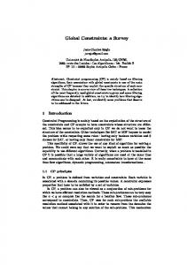
6. DISCUSSION 6.1. Implications for Antimatter and γ-rays We also use our best-fit model to calculate secondary antiprotons, electrons, positrons, and diffuse γ-rays which were not fitted, but provide a useful consistency check. For this calculation the spectra of CR protons and He were adjusted to the BESS data (Sanuki et al. 2000). Secondary antiprotons were calculated using the same formalism as in Moskalenko et al. (2002). Calculation of secondary electrons, positrons, and diffuse γ-rays is described in Sec. 3. The spectra of secondaries are shown in Figs. 7-9. The primary electron injection spectrum is based on fitting to pre-Fermi electron data (conventional model, Strong et al. 2004; Ptuskin et al. 2006), and is parameterized as a broken power law with indices 1.6/2.5 below/above 4 GeV and a steepening (index 5) above 2 TeV, and normalized to the Fermi data at 25 GeV (Ackermann et al. 2010). The plot for the CR electron and positron spectrum is shown separately in Fig. 7 and compared to relevant measurements, while the plot for total leptons (electrons plus positrons) is displayed in the left panel of Fig. 8. Even though the total electron and diffuse emission data were not fitted, they agree well with our best-fit model predictions. The positron fraction, shown in the right panel of Fig. 8, does not agree with the PAMELA data (Adriani et al. 2009), but this was expected since secondary positron production in the general ISM is not capable of producing an abundance that rises with energy. Antiprotons, shown in Fig. 9, also not fitted, present an interesting example where the intensity at a few GeV is significantly underpredicted by the reacceleration models. As has been already shown (Moskalenko et al. 2002, 2003), the antiproton flux measurements by BESS taken during the last solar minimum, 1995–1997 (Orito et al. 2000), are inconsistent with reacceleration models at the 40% level at about 2 GeV, while the stated measurement uncertainties in this energy range are 20%. The reacceleration models considered are conventional models, based on local CR measurements, Kolmogorov diffusion, and uniform CR source spectra throughout the Galaxy. Models without reacceleration that can reproduce the antiproton flux, however, fall short of explaining the low-energy decrease in the secondary/primary nuclei ratio. To be consistent with both, the introduction of breaks in the diffusion coefficient and the injection spectrum is required, which may suggest new phenomena in particle acceleration and propagation. An inclusion of a local primary component at low energies, possibly associated with the Local Bubble, can reconcile the data (Moskalenko et al. 2003). Figure 9 shows that the reacceleration model underproduces antiprotons in the GeV range by ∼30% also compared to the PAMELA data taken during the current solar minimum (Adriani et al. 2010). On the other hand, high-energy PAMELA data agree well with the predictions, which may suggest that the excess over the model predictions at low energies can be associated with the solar modulation. Since reacceleration is also most important below a few GeV, at present it does not appear possible to distinguish these effects. However, a more systematic analysis which includes evaluation of other propagation models may help and will be carried out in a future work.

15

10−9

10−10

68%, 95% regions Φ=0 MeV Φ=500 MeV Φ=1000 MeV

10−11 102

103

104

105

E (MeV)

F IG . 9.— Antiproton spectrum for our best-fit CR parameters, with three different representative solar modulation potentials together with recent data. Note that the error band has not been modulated. The modulated curve for Φ=500 MV is most appropriate for the BESS 1995–1997 flight (Orito et al. 2000) and PAMELA current solar minimum data (Adriani et al. 2010), while the BESS-Polar flight of 2004 (Abe et al. 2008) corresponds to the higher level of solar activity. The data shown here have not been fitted.

The most recent reported results from this approach are in Maurin et al. (2010) and Putze et al. (2010a), which used χ2 and MCMC techniques to analyze a wide range of semianalytical models. The nearest case to ours is their diffusion/reacceleration model where they found δ = 0.23 − 0.24, vAlf = 70 − 80 km s−1 and zh = 4 − 6 kpc. Better fits are found with convection included as well, with a smaller vAlf , but this requires a very large δ = 0.8 − 0.9. In contrast, we find a more plausible range of values for the diffusion/reaccleration model (however we do not consider convection here). We also note that they assume an injection spectrum that is a single power-law in rigidity, which also includes a factor of β ηS , ∼β ηS ρ−ν (Putze et al. 2010b). In the case of proton and He injection spectra in the reacceleration model (their Model II) they use ηS ≈ 1. This is equivalent to our break in the injection spectrum provided the diffusion coefficient has a form Eq. (5). For heavier nuclei, C to Fe, their injection spectrum has ηS ≈ 2, which compensates for the large values of the vAlf in their fits. Therefore, their best fit parameters (e.g., vAlf ) are not equivalent to ours and are dependent on a particular choice of the injection spectrum. Their conclusion that they do not need a break in the injection spectrum is thus significantly overstated as they need an ad hoc factor β ηS with index ηS different for different groups of nuclei. 7. CONCLUSIONS For the first time, we have shown that a full Bayesian analysis is possible using both MCMC and nested sampling despite the heavy computational demands of a numerical propagation code. Furthermore, our analysis also returns the value of the Bayesian evidence, which could be used to rank different propagation models in terms of their performance in explaining the data. While we have not investigated this possibility here, we leave this topic for a dedicated discussion in a forthcoming publication. The present study provides not just best-fit values for the propagation parameters but, more importantly, associated uncertainties which fully account for correlations among param-

16

Trotta et al.

Eγ2 Jγ (cm-2 s-1 sr-1 MeV)

0° ≤ l ≤ 360°, 10° ≤ |b| ≤ 20°

10-3

Fermi-LAT Total Model + Isotropic + Sources Isotropic + Sources Total Model Bremsstrahlung Pion-decay Inverse Compton 10-4 102

103 Eγ (MeV)

104

F IG . 10.— Diffuse γ-ray spectra for 10◦ ≤ |b| ≤ 20◦ for our best-fit CR parameters compared with Fermi-LAT data for the same region of sky. The Fermi-LAT data along with the unidentified background and source components are taken from Abdo et al. (2009b). The red hatched area represents the systematic uncertainty in the spectrum of the diffuse emission, as given in Abdo et al. (2009b). Note that our best-fit model corresponds closely to that used in Abdo et al. (2009b) to derive the unidentified background and source components. Therefore, the addition of our model to these components is valid. Note that these data have not been fitted.

eters, as well as for experimental and theoretical uncertainties. Such error estimates have been fully propagated to the predicted CRs spectra from the model, thus providing an estimate of the residual uncertainty on the predictions (after fitting), which can be used to assess, e.g., potential inconsistencies between different types of data or for model selection. An important conclusion is that the parameter ranges derived in this study are consistent with previous, less systematic analyses.

A valuable test made possible by our technique is the consistency check of the calculated spectra of other CR species, antiprotons, electrons, and positrons with data. Total electrons agree with the Fermi-LAT spectrum within the systematic uncertainties, see Fig. 10. The calculated spectrum of the Galactic diffuse emission for the mid-latitude range is also in a good agreement with the observations by the Fermi-LAT. The antiprotons are under-predicted, which is a general feature of reacceleration models as we have shown before. The positron fraction is inconsistent with a purely secondary origin of positrons above 1 GeV, confirming the excess above 10 GeV attributed to sources of primary positrons. On the other hand, the predicted positron spectrum is consistent with earlier experiments given their large error bars. We await publication of PAMELA positron data for further model comparison. Because of the pioneering nature of our approach, we have concentrated on just one particular type of model with reacceleration and a power-law diffusion coefficient. Other propagation modes, e.g., convection, are not considered here. Future work will consider these, together with constraints from antiprotons, positrons, and γ-rays. R. T. would like to thank the EU FP6 Marie Curie Research and Training Network “UniverseNet” (MRTN-CT-2006035863) for partial support and the Institut d’Astrophysique de Paris for hospitality. I. V. M. acknowledges support from NASA Grant No. NNX09AC15G. T. A. P. acknowledges support from NASA Grant No. NNX10AE78G. The use of Imperial College High Perfomance Computing cluster is gratefully acknowledged.

APPENDIX A. SUPPLEMENTARY MATERIAL

The Supplementary Material accompanying this paper contains the following files, which can be used to reproduce the results presented in the paper. • Galprop chains.tar.gz: Upon unpacking, this archive contains the 10 MCMC chains used in the paper, and one .info file detailing what information is contained in the chains. • The folder BestFitSpectra contains datafiles with the best-fit spectra from our paper. The files and their contents are described in an accompanying README file. • Galprop definition files are supplied for the best-fit parameter values as well as for the posterior mean values (as per Table 2). REFERENCES Abdo, A. A. et al. 2009a, Physical Review Letters, 103, 251101 —. 2009b, Physical Review Letters, 103, 251101 —. 2009c, Physical Review Letters, 102, 181101 —. 2009d, ApJ, 703, 1249 —. 2010, Physical Review Letters, 104, 101101 Abe, K. et al. 2008, Physics Letters B, 670, 103 Ackermann, M. et al. 2010, Phys. Rev. D, 82, 092004 Adriani, O. et al. 2010, Physical Review Letters, 105, 121101 —. 2009, Nature, 458, 607 Aguilar, M. et al. 2007, Physics Letters B, 646, 145 Aharonian, F. et al. 2009, A&A, 508, 561 —. 2008, Physical Review Letters, 101, 261104 Ahn, H. S. et al. 2008, Astroparticle Physics, 30, 133 Alcaraz, J. et al. 2000, Physics Letters B, 484, 10 Badhwar, G. D., Golden, R. L., & Stephens, S. A. 1977, Phys. Rev. D, 15, 820

Barnes, III, T. G., Jefferys, W. H., Berger, J. O., Mueller, P. J., Orr, K., & Rodriguez, R. 2003, ApJ, 592, 539 Beatty, J. J. et al. 2004, Physical Review Letters, 93, 241102 Berezinskii, V. S., Bulanov, S. V., Dogiel, V. A., & Ptuskin, V. S. 1990, Astrophysics of cosmic rays, ed. Amsterdam: North-Holland, 1990, edited by Ginzburg, V. L. Boezio, M. et al. 2000, ApJ, 532, 653 Chang, J. et al. 2008, Nature, 456, 362 Connell, J. J. 1998, ApJ, 501, L59 de Nolfo, G. A. et al. 2006, Advances in Space Research, 38, 1558 Dermer, C. D. 1986a, ApJ, 307, 47 —. 1986b, A&A, 157, 223 Donato, F., Maurin, D., & Taillet, R. 2002, A&A, 381, 539 Duvernois, M. A., Simpson, J. A., & Thayer, M. R. 1996, A&A, 316, 555 Engelmann, J. J., Ferrando, P., Soutoul, A., Goret, P., & Juliusson, E. 1990, A&A, 233, 96

Constraints on cosmic ray Feroz, F., & Hobson, M. P. 2008, MNRAS, 384, 449 Feroz, F., Hobson, M. P., & Bridges, M. 2009, MNRAS, 398, 1601 Florinski, V., Zank, G. P., & Pogorelov, N. V. 2003, Journal of Geophysical Research (Space Physics), 108, 1228 Gelman, A., & Rubin, D. B. 1992, Statistical Science, 7, 585 George, J. S. et al. 2009, ApJ, 698, 1666 Gleeson, L. J., & Axford, W. I. 1968, ApJ, 154, 1011 G´orski, K. M., Hivon, E., Banday, A. J., Wandelt, B. D., Hansen, F. K., Reinecke, M., & Bartelmann, M. 2005, ApJ, 622, 759 Hams, T. et al. 2004, ApJ, 611, 892 Heber, B., Fichtner, H., & Scherer, K. 2006, Space Science Reviews, 125, 81 Jaynes, E. T., & Bretthorst, G. L. 2003, Probability Theory, ed. Cambridge University Press Kamae, T., Abe, T., & Koi, T. 2005, ApJ, 620, 244 Kelner, S. R., Aharonian, F. A., & Bugayov, V. V. 2006, Phys. Rev. D, 74, 034018 Langner, U. W., Potgieter, M. S., Fichtner, H., & Borrmann, T. 2006, ApJ, 640, 1119 Lukasiak, A., McDonald, F. B., & Webber, W. R. 1999, in 26th Int. Cosmic Ray Conf. (Salt Lake City), Vol. 3, , 41 Mashnik, S. G., Gudima, K. K., Moskalenko, I. V., Prael, R. E., & Sierk, A. J. 2004, Advances in Space Research, 34, 1288 Maurin, D., Donato, F., Taillet, R., & Salati, P. 2001, ApJ, 555, 585 Maurin, D., Putze, A., & Derome, L. 2010, A&A, 516, A67 Maurin, D., Taillet, R., & Donato, F. 2002, A&A, 394, 1039 Moskalenko, I. V., & Mashnik, S. G. 2003, in 28th Int. Cosmic Ray Conf. (Tsukuba), Vol. 4, , 1969 Moskalenko, I. V., Mashnik, S. G., & Strong, A. W. 2001, Proc. 27th Int. Cosmic Ray Conf. (Hamburg), 5, 1836 Moskalenko, I. V., Porter, T. A., & Strong, A. W. 2006, ApJ, 640, L155 Moskalenko, I. V., & Strong, A. W. 1998, ApJ, 493, 694 —. 2000, ApJ, 528, 357 Moskalenko, I. V., Strong, A. W., Mashnik, S. G., & Ormes, J. F. 2003, ApJ, 586, 1050 Moskalenko, I. V., Strong, A. W., Ormes, J. F., & Potgieter, M. S. 2002, ApJ, 565, 280 Moskalenko, I. V., Strong, A. W., & Porter, T. A. 2008, in 30th Int. Cosmic Ray Conf. (Merida), Vol. 2, , 129 Moskalenko, I. V., Strong, A. W., & Reimer, O. 2004, in Astrophysics and Space Science Library, Vol. 304, Cosmic Gamma-Ray Sources, ed. K. S. Cheng & G. E. Romero, 279 Mukherjee, P., Parkinson, D., & Liddle, A. R. 2006, ApJ, 638, L51 Orito, S. et al. 2000, Physical Review Letters, 84, 1078 Panov, A. D., Sokolskaya, N. V., Adams, Jr., J. H., & et al. 2008, in 30th Int. Cosmic Ray Conf. (Merida), Vol. 2, , 3 Parker, E. N. 1965, Planet. Space Sci., 13, 9

17

Porter, T. A., Moskalenko, I. V., Strong, A. W., Orlando, E., & Bouchet, L. 2008, ApJ, 682, 400 Porter, T. A., & Strong, A. 2005, in 29th Int. Cosmic Ray Conf. (Pune), Vol. 4, , 77 Potgieter, M., & Langner, U. 2004, Annales Geophysicae, 22, 3729 Potgieter, M. S. 1998, Space Science Reviews, 83, 147 Press, W. H., Teukolsky, S. A., Vetterling, W. T., & Flannery, B. P. 1992, Numerical recipes in FORTRAN. The art of scientific computing, ed. Press, W. H., Teukolsky, S. A., Vetterling, W. T., & Flannery, B. P. Ptuskin, V. S., Moskalenko, I. V., Jones, F. C., Strong, A. W., & Zirakashvili, V. N. 2006, ApJ, 642, 902 Ptuskin, V. S., & Soutoul, A. 1998, A&A, 337, 859 Putze, A., Derome, L., & Maurin, D. 2010a, A&A, 516, A66 Putze, A., Maurin, D., & Donato, F. 2010b, A&A, in press (ArXiv: 1011.0989) Ruiz de Austri, R., Trotta, R., & Roszkowski, L. 2006, JHEP, 5, 2 Sanuki, T. et al. 2000, ApJ, 545, 1135 Seo, E. S., & Ptuskin, V. S. 1994, ApJ, 431, 705 Silberberg, R., Tsao, C. H., & Barghouty, A. F. 1998, ApJ, 501, 911 Skilling, J. 2004, in American Institute of Physics Conference Series, Vol. 735, American Institute of Physics Conference Series, ed. R. Fischer, R. Preuss, & U. V. Toussaint, 395–405 Skilling, J. 2006, Bayesian Analysis, 1, 833 Stecker, F. W. 1970, Ap&SS, 6, 377 Stephens, S. A., & Badhwar, G. D. 1981, Ap&SS, 76, 213 Strong, A. W., & Moskalenko, I. V. 1998, ApJ, 509, 212 —. 2001, Advances in Space Research, 27, 717 Strong, A. W., Moskalenko, I. V., & Ptuskin, V. S. 2007, Annual Review of Nuclear and Particle Science, 57, 285 Strong, A. W., Moskalenko, I. V., & Reimer, O. 2000, ApJ, 537, 763 —. 2004, ApJ, 613, 962 Strong, A. W., Porter, T. A., Digel, S. W., J´ohannesson, G., Martin, P., Moskalenko, I. V., Murphy, E. J., & Orlando, E. 2010, ApJ, 722, L58 Tibaldo, L., Grenier, I. A., & for the Fermi LAT Collaboration. 2009, ArXiv: 0907.0312 Trotta, R. 2007, MNRAS, 378, 72 —. 2008, Contemporary Physics, 49, 71 Trotta, R., Feroz, F., Hobson, M., Roszkowski, L., & Ruiz de Austri, R. 2008, JHEP, 12, 24 Trotta, R., Feroz, F., Hobson, M. P., Roszkowski, L., & Ruiz de Austri, R. 2008, JHEP, 12, 024 Vladimirov, A. E. et al. 2010, Computer Physics Comm., submitted (ArXiv: 1008.3642) Webber, W. R., & Soutoul, A. 1998, ApJ, 506, 335 Webber, W. R., Soutoul, A., Kish, J. C., & Rockstroh, J. M. 2003, ApJS, 144, 153 Yanasak, N. E. et al. 2001, ApJ, 563, 768