Florida Institute of Technology. MELBOURNE, FLORIDA. ABSTRACT. The real time estimation of ship motion is considered in this paper. The problem is viewed ...
NEURAL NETWORK APPLICATION TO SHIP POSITION ESTIMATION
D.G.Lainiotis, K.N. Plataniotis, Dinesh Menon, C.J. Charalampous Florida Institute of Technology MELBOURNE, FLORIDA
ABSTRACT
model equations are derived from the ship motion spectral density which corresponds to a particular seaship condition, the wave excitation input, and a gaussian random noise as driving input. In other words the seastate magnitude, the ship speed, the ship heading with respect to the waves, and the disturbance pattern of the sea waves are incorporated in the model 151, [6].
The real time estimation of ship motion is considered in this paper. The problem is viewed as an estimatiod prediction problem for partially unknown systems. A neural estimator based on a dynamic recurrent neural network is considered. The model that describes the ship motion dynamics is presented, and the neural algorithm is tested and evaluated via extensive simulations. The results show that the new algorithm has excellent performance, and a significant saving in computational time is achieved.
In this paper the estimation of the ship motion based on a linear state-space model that includes the waveexcitation input is proposed. Specifically, the paper is organized as follows. In Section 11, the general formulation of the ship motion dynamics is presented. In Section 111, the neural solutions are tested in extensive simulations on the ship motion model, and are compared with the conventional methods. Conclusions are given in Section IV.
I. INTRODUCTION The accurate on-line estimation of ship motion is essential to many ship related problems such as ship steering [l], dynamic positioning [2], marine oil exploration [3], off shore platforms, and aircraft landing and take-off [41. Based upon predicted ship motion, the necessary control commands for the control of highly qualified ships like hovercrafts are calculated and generated. Ship motion prediction is also essential when accurate control of position mechanisms for guns or missiles is required. When tracking of a maneuvering target is the objective, there is a considerable amount of delay in transmitting information regarding the motion to the position mechanism. It is obvious that accurate predictions are required before an appropriate tracking command can be issued [31.
II. SHIP MOTION DYNAMICS The motion of the ship can be described by a set of differential equations. As it was mentioned above, the model depends on the sea-state magnitude, the ship speed and the ship heading with respect to the waves. For a rigid ship travelling with a constant forward speed and in the direction which makes an arbitrary angle with regard to sinusoidal waves, its motion can be described by a set of second-order linear differential equations of the form: oq(t) +bi(t) +cq(r) = { ( l )
In the past a lot of studies have been carried out for the solution of the ship positioning problem, most of them utilizing the Kalman Filter approach, or other leastsquares estimation methods [ 1],[3]. However the design of a statistical estimator like the Kalman Filter requires the definition of a linear model describing the motion of the ship. More specifically, it requires a state-space representation of this motion. In most of the cases, the
(1) where, q(t) represent a vector of surge, sway and heave motions or variations of roll, pitch and yaw orientations, t ( t ) represents the sea-wave excitation, and a,b,c are constants that represents the virtual mass, damping and restoring stiffness, and are determined by the dimensions and shape of the ship.
1-384
0-7803-1385-2/93/$3.00 (B 1993 IEEE
The above linear model can be obtained using the power spectral density function under different sea-wave excitation [5]. The most important part of the equation is representation of the periodlc sea-wave excitation. The wave excitation can be approximated by the superposition of sinusoidal waves [6]. c(1)
(6) where, x(t) is the state vector which represents the ship motion. It is a 2 x 1 vector defined as follows:
= EAl sin(w, l+b,)
(2) where, A, is the amplitude of wave excitation, w,, the frequency and b,, the phase of each different wave.
In most of the cases, the amplitude and the frequency of the waves are considered to be time-invariant. When the ship is moving with forward speed, there exists a certain relation between the ac tual wave frequencies, and the frequencies encountered by the ship[6]. Following this relation, the direct influence of the waves on the ship is given as follows:
(7) Ce(t) is the truncated wave excitation input, w(t) is the state random noise, z(k) is the discrete measurement vector and v(k) is a random noise which corrupts the measurements.
(3)
62
w . = w -. 2 el
i
g
'
U
'
cos ( x )
(4) where, w e i is the transformed wave frequency, v is the forward speed of the ship, x is the angle between the ship hcading and the wave direction, and g is the standard gravitational acccleration. Moreover since the energy of each individual wave component rapidly decreases as the frequency of the wave increases, the above expression can be simplified further. Truncating the high frequency components the expression takes thc following rorm: N
5,(1)
=
1 Ai.sin(wei.l+Di) i= 1
(5) It is reported in numerous studies [11,[51,[61,[7] that a value of 3 for N, is sufficient to approximate the wave excitation input, in the caw of small ships. After all the approximations and tranciformations, the equation for the ship motion in the equivalent state space representation can be writl.en as follows:
The position and velocity of the ship are usually measured by on-board sensors. Since all the states are not measurable, and the measurements always contain noise, filters are employed Lo estimate the actual position of the ship. The objective is to obtain the optimal, stale estimate i ( k / k ) of the state x(k/k), in the mean square scnsc, given the measurement record, Z(k)=( z(l),z(2),.., z(k)).
III. SHIP POSITION ESTIMATORS In the past K a h n Filter based techniques, or other statistical filters have been used in connection with state space models in order to provide meaningful and accurate estimates of the ship motion. If the sea-wave excitation (sea condition) is known in advance, and all other dynamic and statistical specifications of the above model meet h e assumptions of the Kalman Filter, then this filter is the optimal estimator and provides the most accurate estimate. However tile sea condition is not always known in advance to thc designer of the filter. In this situation, when a mismatch occurs between the actual model and the model used by the designer, the Kalman filter fails. A more robust statistical filter, namely the Adaptive
Lainiotis Filter [8],[9], was successfully used in this situation. Unlike the Kalman Filter, this new filter, due to its adaptive nature, identifies in real time, the actual model and provides the appropriate solutions [8],[ 111. Recently, neural networks have been used to estimate
1-385
assuming initial state estimate, n(O/O) = 0, and initial covariance, P(0K)) = loo.
states of dynamic systems [12],[13],[14]. In this paper, a neural network is used to provide the ship motion estimates. The estimator is a multilayer recurrent neural network, trained using back-propagation technique, to provide estimates of the ship position.
Neural estimator: recurrent, multilayer network
-network topology: The following simulation experiments are performed:
two input nodes: the current and the previous neural output are used as input signals two output nodes: the estimates of the system states. The neural network has so many output nodes, as the states of the model two hidden layers with 10-10 hidden nodes respectively
SIMULATION I: In this experiment, the neural estimator is compared with the optimal Kalman filter. It is supposed for comparison purposes that the dynamic model is completely known, and the statistical Kalman filter is matched to the actual dynamic and statistical model of the ship dynamics. Although this situation is highly unrealistic, this comparison is made to evaluate the performance of the neural estimator, viz. a viz., the inaccessible performance of the optimal Kalman filter. The experimental set-up is given below:
-learning parameters: learning rate: 0.005, momentum: 0.2
-Training procedure:
System Model:
backpropagation training algorithm the network knows the actual states of the model during the training phase. The target vector is the actual state vector the network tries to minimize the square error between the current output and the target vector The training data set is produced by running the system equations. The training set consists of 150 input/output
Pairs (z(k), x&)) The test data record consists of a sequence of data points produced separately from the training record the training procedure is terminated if the training error tolerance is less than 0.01 or if the number of iterations of the training set is more than 5000
where,
mi),
ati-l = A.cos ati = A.sin (bi). The amplitude of the wave excitation input, Ad.5, with a constant excitation frequency, wi = d4; different phases are, bl=2~/3, b2=n/3, q=d6. Q=0.25 and R=0.1, are zero-mean, white, gaussian, plant and measurement noise covariances,respectively.
Observations:
In Figs.1-3, the performance of the Kalman Filter in the estimation of the position and the normalized e m r over 100 Monte Carlo trials are given. The average error in the performance during the Monte Carlo simulation is calculated using the following performance index:
In order to estimate the states of the above model, the following estimators are used in this first experiment:
Statistical estimator: K a l m n filter The Kalman Filter is matched to the above dynamic and statistical model. All the quantities of the state-space model is assumed to be known a-priori to the filter designer. Moreover, the filter starts its recursive cycle
MS E =
-.1
mc
C
mc
. r=l
{ ~ ( k- )n ( k / k ) } / ( x ( k ) )
(10) From the figures it is obvious that the Kalman Filter
1-386
performs very well, when all the parameters of the dynamic and statistical model are known. In Figs.2 and 3, the performance of the neural estimator in the estimation of the ship position and its error over 100 Monte Carlo runs, using the same performance index shown above, is given. In summary, the following conclusions can be drawn: for a linear, gaussian model, if the underlying statistics and dynamics of the phenomenon is completely known to the estimator, the Kalman filter provides the optimal results. the neural estimator performs similar to the optimal filter even though it is a nonlinear structure applied to a linear, gaussian model. SIMULATION 11: It was mentioned in the introduction that many times it is more important to predict ahead the position of the ship, rather than estimate its current position. This will be the subject of the second experiment. In particular, we arc interested in comparing the performance of a neural predictor, with that of the Kalman predictor. The model used in the experiment is the same twodimensional state-space model used in the previous one. The following two estimators / predictors are compared:
Statistical predictor: Kalman Jilter Two Kalman filters are used in this simulation experiment. The first one is matched to the actual dynamic model. All the quantities of the dynamic model is supposed to be known to the designer. The second Kalman filter docs not know the exact dynamic model. More specifically in its design another variation of the wave excitation has bcen assumed. Both the filters assume that the measurement noise is gaussian, zero mean, with variance, R = 0.1. The initial state is assumed to be gaussian, with the initial estimate, a(O/O) =0, and initial covariance, P(O/O) = 100. The objective for each of them is the prediction of the ship position two seconds ahead.
one output node: the prediction of the next measurement value three hidden layers with 10-10-10hidden nodes respectively -learning
parameters:
learning rate: 0.001, momentum: 0.1 -Training procedure: backpropagation training algorithm the network does not know the actual states of the model during the training phase. The target vector is again a measurement value the network tries to minimize the square error between the current output and the target vector the test data record consists of a sequence of data points produced separately from the training record the training procedure is terminated if the training error tolerance is less than 0.01 or if the number of iterations is more than 5000
Observations: As was expected, the neural predictor performs better than the mismatched Kalman predictor, despite the minimal information required for its training. The prediction of the network, is shown in Fig. 4. However when the model that describes the wave excitation is completely known, the Kalman filter provides the optimal predictions. The perfomance of the two Kalman predictors and the corrcsponding errors over 100 Monte Carlo runs are given in Figs. 5-8. These results lead us to the following conclusions: the neural predictor requires very little information about the nature of the model, and provides best predictions, with total ignorance of the actual dynamic and statistical model. the statistical predictor (Kalman filler) does not perform as well, and provides suboptimal solutions when a mismatch between the actual model and the one used in the design exist. The comparative graphical representations, shown in Figs. 7 and 8 confirm the above conclusions.
Neural predictor: recurrtmt multilayer network
-network topology: five input nodcs: the current and the four previous measurlm” are used as input signals
1-387
Vol. OE-15, NO. 3, July 1990,pp. 244-250.
IK CONCLUSIONS
[7] B. Friedland, “Estimating angular velociry from
The real time ship motion estimation and prediction was considered in this paper. The approach taken, was to design a neural network based estimator, that can handle more realistic scenarios about the underlying physical model. A comparison with the most widely used statistical Kalman filter estimator, was made. Simulation experiments were carried out in order to assess the performance. In the ship motion prediction problem, the neural network predictor shows excellent performance, though it was derived using minimal information about the dynamics of the model.
output
of rate
integrating
gyro”, IEEE
Transactions on AES-11, July 1975, pp. 551-555. [8] D.G. Lainiotis et al., “Real time ship motion estimation using Lainiotis
Filters”, IFAC
Workshop, CAMS-’89, Expert Systems in Marine Automation, pp. 293-301,1989. [9] D.G. Lainiotis, “Optimal adaptive estimation: Structure and parameter adaptation”, IEEE
REFERENCES
Transactions on Automatic Control, Vol. AC-16, pp. 160-170, April 1971.
[l] R.E. Reid, A.K. Tugcu, B.C. Mears, “The use of
D.G.
Lainiotis, “Partitioning: A
unifying
wave filter design in Kalman Filter state
framework for adaptive systems. I-Estimation”,
estimation for the automatic steering problem of
Proceedings of IEEE, Vol. 64,pp. 1126-1142,
a tanker in a seaway”, IEEE Transactions on
August 1976.
Automatic Control, Vol. AC-20, No. 7, pp. 917-
D.G.
922,1984.
Gianakopoulos, S. Kctsikas, “Heal time ship
[2] T. M. Weiss. T. W. Devries, “Ship motion
Lainiotis,
C.J.
Charalampous,
P.
motion estimation”, Proceedings Oceans ‘92, pp.
measurement filter design” , IEEE Joumal of
283-287, Newport, Rhode Island, 1992.
Ocean Engineering, Vol. OE-2, No. 4, October
D.E. Rumelhart, J.L. McClelland, “Parallel
. 1977, p ~ 325-330.
Distributed Processing: Explorations into the
[3] M.S. Triantafyllou, M.Bodson, M. Athans, “Real
Microstructure of Cognition, bbl. I ” , M.I.T.
time estimation of ship motion using Kalman
Press, 1986.
Filtering technique”, IEEE Joumal of Ocean
[13] J.P. De Gruyenaece, H.M. Haffer, “A comparison
Engineering, Vol OE-8, pp. 8-20, January 1983.
between Kalman Filters and recurrent neural
[4] M.M. Siolar, B.F. Doolin, “On thefeasibility of real
networks”, Proceedings of UCNN-92, Vol. IV,
time prediction of aircraft carrier motion at sea”,
pp. 247-251, 1992.
IEEE Transactions of Automatic Control, Vol.
[14] A.J. Kanekar, A. Feliachi, “State estimation using
AC-28, pp. 350-356, March 1983.
artificial neural nehvorks” ,Proceedings of IEEE
[5] R. Bhattacharyya, “Dynamics of Marine Vehicles”, Wiley N.Y.,1978.
Systems and Engineering Conference, pp. 552556,1990.
[6] J.C. Chung, Z. Bien, Y.S.Kim, “A note on shipmotion prediction based on wave-excitation input estimation”, IEEE Journal of Ocean Engineering,
1-388
Fig. 1 Ship position estimation: ncuml estimator
Wg. 5 Ship position prcdicnon : Matched Kalman filter U"
.ol*nll.*-.I"Lmtl
-s
. I
t
I.
I
.
I.
'i LI
I
I
0
9 ,
I. I I -
6.
1.
LL " " Fig. 6 Ship position prediction :Mismatched Kaiman filter I'
Fig 2 Ship positlon estunation: Kalman filter
!
I
"
>.
,.
Fig. 3 Estimation , Normalized error: Comuarauve evaluatton ,100 MC Fig. 7 PredicuonNormaliztd error Comparative evaluation 100 MC ..m,010tz I.,,
,011110
I-
yuol
' I '
Fig. 1 Ship position prediction: neural predictor
Fig. 8 PredicuonNormalizcd error Comparative evaluation 100 MC Neural oredictor vs. Mismatched Kalman filter
1-389
DEVELOPMENT OF A SIX DEGREE OF FREEDOM BUOY DESIGN AND ANALYSIS PROGRAM WITH VALIDATING DATA W. A. Venezia Ocean Systems Development Corp. 375 N.W. 35th Lane Boca Raton, Florida 3343 1 (407) 45 1-7226
A. M. Clark Harbor Branch Oceanographic Inst. 5600 Old Dixie Highway Fort Pierce, FL 34946 (407) 465-2400
Abstrod-A six degree of freedom buoy design and analysis program is given. The buoy program extends original work published by the Woods Hole Oceanographic Institution for roll and heave response of free floating axisymetric bodies. The program predicts the probable amplitude of buoy displacement, velocity, acceleration, and jerk for heave, surge, and sway, motions and probable amplitude of roll, pitch, and yaw angular displacements, velocities, and accelerations. Given is an overview of the equations of motion, simplifying assumptions, and a description of the computational method. The paper contributes limited verification of the computational method with a summary of computer predictions and experimentally obtained data on buoy motion. The data 011 motionn is obtained from buoys designed with specific buoy motion requirements. Experimental data is given for various sea states and buoy types
.
I. INTRODUCTION
Modern oceanographic measurement techniques often require highly stable platforms with predictable levels of motion[1,2]. Modem air sea interaction studies depend on at-sea experimental model verifications to test and evaluate emerging theories in a wide variety of Ocean sciences. Experiments range from global heat flux, including prediction of momentum exchange in the presence of waves, to the understanding of radio wave propagation over the sea. The advent of the personal computer (PC) provided design engineers with a computational machine that allows for rapid and convenient solution of many classical engineering problems. Off the shelf software is available to solve many of the typical problems encountered in fluid mechanics, solid mechanics and dynarmcs. Ocean engineers seeking to solve complex problems related to the ocean environment are developing their own personal computer based s o h a r e to satisfy system requirements and solve design conflicts[3]. Typical programs include static and dynamic cable, buoy, and towed systems problem solvers. With an increasing number and variety of computer models available it is now more important than ever to have applicable, high quality, well understood data for validating emerging computer codes.
K. F. Schmitt Science Applications International Corp. 10260 Campus Point Drive San Diego, CA 92121 (619) 546-6369
Accurate computer aided tools for the design and analysis of moored and free floating buoy systems require full scale validation and refinements until the user has confidence the program is generating realistic output. Ocean Systems Development Corporation (OSDC) was founded to provide high quality ocean engineering products and services to the maritime industry. OSDC supports theoretical design studies leading to innovative oceanographic instrumentation and stabilized instrument platfoms while providing experienced technical support personnel for the solution of practical problems related to the ocean environment The OSDC six degree of freedom (6DOF) computer solution for free floating buoys presented here was developed over the past twelve years from ideas given in original work published by The Woods Hole Oceanographic Institution (WHOI)[4]. The WHO1 reports present an analysis method and FORTRAN computational code designed to run on a main frame computer for the heave, roll, and pitch response of free floating bodies of cylindrical shape. We extended the work to include surge, sway, and yaw and now have a working code written in Microsoft QBasic for a PC. The program predicts the probable amplitude of displacement, velocity, acceleration, and jerk for heave, surge, and sway, motions and probable amplitude of roll, pitch, and yaw angular displacements, velocities, and accelerations. We compare the output of the code to the response of three buoys built using the code as a design tool. The data we draw on is separate deployments. The deployments are; a 10 m spar at Lock Linnie, Scotland, a 27 m spar off Kauai, Hawaii ,and a 2 m diameter tomdal buoy off Fort Pierce, Florida. The 6DOF buoy design and analysis program was used in each case to predict motions in the design cycle. In each case the buoy motion data was obtained from a strap down motion monitoring package onboard the buoy. Sea state spectral data corresponding to each set of buoy motion data was experimentally obtained from either a wave staff, a wave rider, or a subsurface pressurdwater velocity sensor. To increasing extents, the predicted and measured buoy response is given.
1-390
0-7803-1385-2l93/$3.00 @ 1993 IEEE