encountered in applying these estimPtes are discussed. I. INTRODUCTION. T HE CLASSICAL PROBLEM in array signal processing is to determine the location ...
PROCEEDINGS OF THE IEEE, VOL. 70, NO. 9, SEPTEMBER 1982
1018
The Application of Spectral Estimation Methods to Bearing Estimation Problems
Invited Paper
Abmucr-The equivalence between the problem of determining the bearing of a rndirtiq source with an may of & M O and ~the problem of estimating the spectrumof a signal is demonstrated. Modem spectral estimation algorithms am derived within thecontext of a m y procedng wing an Plgebraic EmphPsis is placed on theproblem of determining the bearing of a swnd source with an array. Special issues
approach.
encountered in applying these estimPtesare discussed
I . INTRODUCTION
T
HE CLASSICAL PROBLEM in array signal processing is to determine the location of a source which is radiating energy. A single array is used to estimate the direction of the source relative to the location of the array. The outputs of several such arrays, which are separated from each other, are then used t o determine location. The direction estimation problem is of interest here; it is shown later that this problem is mathematically equivalent to estimating the Fourier transform of the radiation field. The recurrent example used in this paper be thedetermination of the bearing of an
acoustic Source with an array;problem is referred to as the passivesonar problem. In this problem, the signal-to-noise ratioencountered in practice of a single sensor’s output is usually small (on the order of 0 dB). Consequently, spectral estimation algorithms capable of determining the spectrum of a signal measured in the presence of significant noise are of special interest. It is shown here that many of the so-called “modem” algorithms can be derived in a unified way as the solution of a constrained optimization problem. The intent of this paper is to present these algorithms in this framework and t o interpret the results in the context of array processing problems. While equivalent to estimating a spectrum, special issues are introduced when these procedures are applied to the bearing estimation problem. Most of these algorithms have been derived elsewhere; however, some new resultsare presented. We assume that a plane-wave signal s(r, x) is propagating in a medium at speed c in the direction -ko (Fig. 1). An array of M sensors is present in the medium. Each sensor is assumed to record the acoustic field at its spatialpositionwithperfect fidelity. The waveform measured at the spatial position Zm of the mth sensor is denoted by x m ( r ) and is given by
where
Nm(t)
is additive noise and zm ko denotesthedot
l
Fig. 1.Definition of variables involved in array processing. An array of sensora is located in a medium. The origin for the coordinate system of the array canbechosenarbitrarily, b i t is usuallychosen to bethe centroid of the array.The vector Om definesthelocation of themth sensorrelative t o t h i origin. A planewave is shown propagating towardthe array inthedirection -ko. Consequently,the bearing of thesourcerelative to the array is denoted by theunitvector k,
.
product of the vector zm and ko. This noise may be due to disturbances propagating in the medium or t o noise generated internally in the sensor or in the associated electronics. One of the oldest ideas in array processing for determining the bearing of anacoustic source (i.e., ko) is beamforming. Here, the outputs of the sensors are summed with weights and delays to form a beam y ( r ) . y ( t )=
am x m (t
- Tm 1.
(2)
m
The idea behind beamforming is to align the propagation delays of a signal presumed t o be propagating in a direction -Lo so as to reinforce it. Signals propagating from other directions and the noise are not reinforced. For example, if the sensor delay Tm is ideally adjusted t o compensate forthe signal delay (zm ko)/c, the signal would be completely reinforced. The delayed output of each sensor would be
-
weights (am = 1) y ( t ) = M s ( t ) + C N , ( t - Tm).
Manuscript received May 5, 1982. ThL workwassupportedbythe Office of Naval Research under Contract N00014-81-K-0565. The author is with the Department of Electrical Engineering, Rice University, Houston, TX 11001.
m
the each sensor
Power in Y ( t ) is M1 times that measured at while the noise power is increased by only a factor
0018-9219/82/0900-1018$00.75 0 1982 IEEE
JOHNSON:BEARINGESTIMATIONPROBLEMS -S8-48 -38 -28 -18
-00
8
18
1019 20
30 48 58
-18O
8
3 -20: 1
t
beam is proportional to the spatial Fourier transform of the quantity a, exp {+j(2nf/c)z, ko}, a sequenceconsisting of signal andbeamformingparametersevaluated atthe spatial positions . ,z The spatialfrequency variable is therefore k ( f / c ) . As c =fX, this variable can be written as k f i . For example,consider a lineararray of equallyspacedsensors. Then , z = mdi,, where i, is the unit vector in the x-direction, and d is thespacingbetweensensors.Then z , *Ao = md sin Bo where Bo is the angle of the direction of propagation from the array broadside. Equation ( 4 ) becomes ~ ( fk), = ~ ( f ) a, exp {-j2n(md/h)(sin e - sin e,)}.
(5)
rn
-2el
t
In a circular array with M sensors equally spaced on a circle of ,z = r cos (2nm/M)i, + radius r, the sensorlocationsare r sin ( 2 n m / M ) i y . Then
{
[
exp -iZn(r/X) cos ( 2 - e~) - cos
-38 -98
l
~
l
~
-58 -48 -3-20
l
-le
~
8
l
~
2818
l
38 48
~
sa
l
~
w
BEARING-deg
Fig. 2. Results of the application of various spectral estimation algorithms. A linear array of ten equally spaced sensors is receiving a single signal coming from an angle of zero degrees. The sensor spacing is h / 2 . The sensorsignal-to-noiseratio ( u : / u i ) is O.dB.The spatial correlationmatrix is givenby (11). (a)Bartlettestunate. (b) Maximum-likelihoodestimate. (c) Linear-predictiveestimate (m, = 0). The referenceamplitude in each part is maximum value of the spectrum in that part.
of M (assuming the noise signals measured by the sensors can be described as mutually uncorrelated processes). More generally, the energy in the beam y ( t ) is computed for many directions-of-look A by manipulating the delays .7, Maxima of this energy as a function of k are assumed to correspond to acousticsources,and the source bearings correspond to the locations of these maxima (Fig. 2). Further insight into beamforming is gained by considering these expressions in the frequency domain [ 11, [ 241. D e f i i g X, (f) to be the Fourier transform of x, ( t ) , the Fourier transform of a beam is given by Y ( f , k)= C a m ~ X P{ - i 2 W / c ) z , *k}X m U )
(3)
rn
-
where the beamforming delay r, is given by (z, k)/c. If, for example, each sensor output consists of a single propagating signal x m(
f ) = S(f) ~ X P{ + i 2 n ( f / c ) z , ko}
~ ( fk), = W )C a m exp {-i277(f/c) zm * (k- ko 1).
(4)
m
Fouriertransform
Y(f)of the
(6)
Thus thecomputation of thisquantity dependsgreatly on array geometry. This frequencydomain analysis also demonstrates several issues important in the evaluation of the performance of a beamformingalgorithm. As ( 4 ) describestheFouriertransl ~ ~ l ~ ~ l ~ l ~ ~ ~ form ofl a sequence, thel spatial spectrum Y c f ,lk) is periodic withperiodone. Forthe linear,equallyspacedarray, this period is d / ( h / 2 ) . If the wavelength of the acoustic signal is such that this quantity is greater than one, diasing occurs: the actual direction-of-propagation can be confusedwith other values of k. On the other hand, if the wavelength is such that this quantity is less thanone,computationswhich usually assume a period of one (such as the fast Fourier transform) will evaluate spatial spectra at frequencies that do not correspond to any physical arrival. The energy in the beam as a function of k is evaluated by computing /I Y c f )1' df anddetermining thelocation of maxima. For simplicity, assume that the signal is narrow-band with all of its energy concentrated at the frequency fo. Thus beam energy P(k) is given by
(7) where X, = c / f o . These results can be formulated in matrix form [ 51, [ 91, [ 2 9 ] . Define thecolumnvector X to containthetemporal Fourier transforms of the array outputs and the elements of column vector A to be
Then Y ( f , k) = A'X where A' denotes the conjugate transpose of A . The vector X is given by X = 0,s + a,N, where S represents a plane-wave signal (S, = exp {+j(2n/X)zm ko}) and N represents noise. The noise is assumed to be statistically independent of the signal. Thesevectors are normalized so that ai and a: denotethe power levels of the signal andnoise, respectively,ateachsensor.Theenergyin the beam when
-
the quantity Y ( f ,A ) is given by
Consequently, thetemporal
(9eo)]}.
PROCEEDINGS IEEE,OF THE
1020
VOL. 7 0 , NO. 9 , SEPTEMBER 1982
The Bartlett estimate is, therefore, given by PBART(k) = E’fRE.
(12)
Assuming that the noise is spatially white, the power in the beam when the array is steered toward the source (k = ko) is found t o be PBART(~O)= M~ O:
d Mn (I)
+ MU:.
(13)
Thus the quantity PBART(&)yields an estimate of the signal power propagating in the direction -k. The previous sectionhas demonstratedthatthe measurement of the bearing of a radiating source by an array is mathematically equivalent to computing a spatial spectrum and determining the location of local maxima. A typical spectrum resulting from conventional beamfonning is shown in Fig. 2(a). This result illustrates the classic problem of array processing. Because of the finite aperture of the array (aperture is defined roughly to be the spatial extent of the array measured in wavelengths), the detail that can be obtainedfromthe spatial frequency response is limited. A source having a welldefined bearing appears to be coming from a dominant but diffused direction as well as from false directionscorresponding t o sidelobes. The sidelobes are due to the equal weighting assumed for eachsensor output (am = 1). Thecomparable result in time-series analysis occurs when a rectangular window is applied to a sinusoidal signal and the spectrum computed.If the weights are tapered, the sidelobes can be reduced but at the expense of a wider mainlobe [ 4 ] . Using this classical approach, increased bearing estimation accuracy can only be obtained by increasing the aperture of the array. This solution is of limited utility as it means increasing the physical size of the array. For this and other technical reasons, modem highresolutionspectral analysis algorithms are being considered instead [231, [291, [391. These methods are usually referred to as adaptive methods as the choices of weights a, and delays r, vary with directionsf-look and the characteristics of the sound field measured by the sensors. In evaluating spectral estimation methods, three criteria are usually used. The first is resolution: the ability of an estimate to reveal the presence of two equal-energy sources which have nearly equal bearings [ 171. When two sources are resolved, two distinct peaks are present in the spectrum;if not resolved, only one peak is found. This defrnition of resolution may not seem t o correspond t o theintuitivenotion of resolution. Rather, a better resolved bearing would seemingly correspond t o a narrower spectral peak. A spectral estimate yielding the sharpest peak usually implies that the bearing has been best resolved. However, the sharpness of apeak can always be increased by raising the spectrum t o a power greater than one. Such a computation does not increase the accuracy to which source bearings can be distinguished. Themore operational definition of resolution is thus preferred: how well cana spectralestimate allow the presence of two sources t o be determined. Spectral estimates are usually normalized in judging resolution so that the value at k = ko equals signal power. For example, the estimates considered here, such as the Bartlett estimate, would be normalized to be proportional t o us’. Note that resolved spectral peaks do not necessarily imply that the peaks are located at the proper bearings. The secondcriterion is therefore the bias of the estimate. When one source is present, the bias (the error in the location of the spectral peak) is usually zero (the estimate is unbiased). However, when two sources are present, the bias is usually nonzero. These two criteria of the “goodness” of a spectrum may con-
-
-30
-ye
-58-48 -3-28
-18
e
18
2e
38 413
se
w
BEARING-de9
Fig. 3. Results of the applications of variousspectral estimation algorithms. The array configuration la identical to that described in the caption to Fig. 2. Two signale are present in the field, one coming from an angle of So, the other from an angle of -5’. The spatial correlation matrix ia given by (30). The sensor signal-to-noise ratio ia 0 dB foreach signal. (a) Bartlett estimate. (b) Maximum-likelihood estimate. (c) Linear predictive estimate (mo = 0).
steered in direction A is given by
P(k)=E[IY(f,k)121 =E[IA’Xl21 =E[A’XX’A] = A’SA (8) where fR=E[XX’] is the spatialcorrelation matrix Of the Sensor outputs. If no noise is present (an = 01,each element of fR is given by
More generally, when noise is present, the spatial correlation matrix is given by fR= a: 9+ 0:Ss’ (10) where 9 is the spatialcorrelationmatrix of the noise. Furthermore, if the noise is spatially white (uncorrelated from sensor to sensor), 2 = 9 so that
R= a:, 4 + a: ss’.
(1 1)
When the weights am are each set t o unity,the so-called Bartlettspectralestimate results (Figs. 2(a) and 3(a)). The steering vector A is set equal to E , where E represents an ideal plane wave that is propagating in the directionsf-look k
JOHNSON:
1021
a c t : goodresolution is oftenobtainedattheexpense of a biased estimate. The third criterion is Variability: the range of bearings over which thelocation of aspectralpeak can be expected to vary. Analytic evaluation of the variability for a Cramer-Rao given spectralestimate is usuallydifficult.The lower bound on the variance is usually used as a benchmark to evaluate the measured performanceof a given method [ 21. 11. MAXIMUM-LIKELIHOOD METHOD Perhaps the most well-known high-resolution array processing algorithm is the so-called maximum-likelihood method first reported by Capon [121, [131, [ 191. The derivation of this method does not correspond to the standard approach used in maximum-likelihoodestimates.Rather, this estimate is derived by finding the steering vector A which yields the minimum beam energy A'%A subject to the constraint thatA'E = 1, where E represents an ideal plane wave corresponding to the direction-of-look. The purpose of the constraint is to fix the processing gain for each directionaf-look to be unity. Minimizing the resulting beam energy reduces the contributions to this energy from sources and/or noise not propagating in the direction-of-look.Thesolution of this constrainedoptimization problem occurs often in the derivation of adaptive array processingalgorithms.Thesolutiontechnique is to use a Lagrange multiplier. We minimize
F = A'%A + a(A'E - (14) 1). The usual approach of setting the gradient of F with respect to A t o zero must be used with caution. The vector A is complex, and the gradientof the conjugateof A cannot be defined. One could evaluate the gradients with respect to the real and imaginary parts, set each result to zero, and solve for A . A simpler approach is to consider A and its conjugate as independent variables rather than the real and imaginary parts [ 161, [38]. When gradientswithrespect to A and A* of F are evaluated, they are conjugates of each other. Setting one of these to zero results in the solution
and thushas units power as doestheBartlettestimate (see (1 3)). Thetruemaximum-likelihoodsolution for A has aform similar to (15). In this approach, a plane wave is presumed to be propagating in the direction -& in the presence of statisticallyindependent Gaussian noise.Thesteeringvector corresponding to maximum-likelihoodestimate of the signal power is easily shown to be AML =
9-l E
E ' PE
Comparing with (15), this vector differs only in the presence of the noise correlation matrix instead of the signal-plusaoise correlationmatrix.Thespatialcorrelationmatrix Iof the noiseinvolvedin this expression is not usually known in practice.Furthermore,thepresence of the signal inthe acoustic field can prevent measurement of it. Capon has termed the estimate P M ~ ( ka )"high-resolution" estimate [ 121.Cox [ 171 hasshown that this method has better resolution properties than the Bartlett estimate (Fig. 3, for example). However, it is not true that this methodhas the best resolution propertiesof any method.
111. LINEAR-PREDICTION METHOD Thelinear-predictivespectralestimate commonly used in timeseriesproblems can also be used in array processing problems [301, [341, [381. As before, let X,, be the Fourier transform of the output of the moth sensor evaluated at the frequency fo. We assume that this value is estimated by a weightedlinearcombination of theoutputs of theother
sensors
X,,=-
a
A = - -%-'E. 2
( E = s),
likelihood beamformer is steered toward the source the maximum-likelihood estimate equals
(21)
amXm m#mo
The linear-predictive method is based on finding the weights
n e quantity a is determined by theconstraintequation A'E = 1;the final solution is then
a, which minimize the mean-squared prediction error
The power in the beam when steered in fp" direction-of-look determined by E is the quadratic form A % A which becomes in this instance (see Fi& 2(b) and 3(b))
Define the column vectorA to be
PML(k) = (&%-'E)-'.
(16)
Theoretical studies of the properties of this estimate rely on a closed-form expression for 3-l. If a matrix is of the form
3=4+BfBc' then itsinverse is given by
3-' = 4 - m e '
(17)
a1
*
,amo-l
am,, amo+l 9
*
~ M - II
T
-
We seek to minimize the quantity E [ IA'Xl'I = A'%A subject to the constraint that a, = 1. This constraint can be written 0. as A'umo = 1 where urn* IS a column vector having the moth element equal to one and the other elements equal to zero. The linear-predictive coefficients are thus seen to be the solution to a constrained optimization problem having the same form as that encountered in the maximum-likelihood method. The solutionis, therefore
I-'%. Forexample, when % is givenby where q)= [ J + ( l l ) , @ = C = u # a n d % = 4 whichresultsin 1 a:,
3-1 =-
I'-
O3
Mu: +o:,
ss'l.
Thus when the noise is spatiallywhiteandthe
maximum-
Using ideasfound intimeseries [ 341, the linear-predictive method corresponds to an all-pole (i.e., autoregressive) model for the signal. In this case, the power spectrumis given by the mean-squaredpredictionerrordividedby themagnitude
PROCEEDINGS IEEE,OF THE
1022
VOL. 70, NO. 9, SEPTEMBER 1982
squared of the spectrum of the predictor coefficients. Consequently,the linear-predictive spectral estimateinthe array case is of the form
which is given by
Figs. 2(c) and 3(c) illustrate examples of this estimate. Using (17), the value of this spectral estimate f o r k = ko and Mu: /uz 1 is easily shown t o be
>>
p~p(ko)=M(M-
1)~:.
This spectral estimate differs from the conventional and the maximum-likelihood estimates in an important way: the value of a peak is proportional to the squure of the signal power. Burg and others [71, 1291 argue that the power of a signal is determinedfrom P~p(k)by the area under the peakrather, than its amplitude. However, if the spectralestimate is modified t o be
-7e
-304
-40
i -58-40 -30 -20
-00
the power estimate when k = ko becomes FLp(k0) = MU:
-10
a
10
20
30 40 50
98
BEARING-deg
+ u:,
Fie. 4. Effect of the choice of
predictionelement m, on thelinearpredictivespectralestimate. The array configuration is described in the caption to Fig. 2 and the signal and noise characteristics in Fig. 3. (a) Sensor signal-to-noiseratio is 0 dB.(b) Sensor signal-to-noise ratio is -10 dB.
With this modification, the resolution properties of the linearpredictive spectralestimatecan be compared with other methods more easily. Linear-predictive spectral estimates for m, = 0 or M - 1 in a linear, equally spaced array have better To minimize the prediction error, one would search for the resolution properties than maximum-likelihood estimates when largest element on the diagonal of % - I . The prediction error the noise is spatially white [ 181, can be smaller for values of m, # M - 1 in many cases. HowThis algorithm has the additional flexibility of the choice of ever, the spectrum corresponding t o this minimum predictionm,, the sensor whose output is being predicted. In time series, error choice is not necessarily “better”thanthatobtained this flexibility is also present although it has not been studied when m, = M 1 or 0. Fig. 4 is an example of this phenomeextensively. There the selection of mo corresponds tothe non. It can be shown that for a linear array of equally spaced choice of sample to be predicted by the other signal samples. sensors, predicting the output of a center element (m, = M/2) In this case, the usual choice is m, = M - 1 so that the past has better resolution properties than those obtained when presamples are used to predict the present one. Thusa causal dicting the output of an end element (m, = M 1 or 0) when signal model is obtained and the remaining choices for m, the source bearings are closely spaced (separated by less than correspond to noncausal models. Causal models are usually one-half abeamwidth) [ 181. However, the opposite result preferred in time series problems. In contrast, causality is not holds when the source bearings are not closely spaced (Fig. 4). a particularly important issue for a spatially distributed array, Fig, 4 also illustrates the nonlinear nature of this spectral and the additional flexibility of choosing which sensor output estimate.Theresolutioncapability of an algorithm can be is to be predicted could yield better spectral estimates, With affected by the signal-to-noise ratio; somealgorithms are affectedmore (m, = 4 in Fig. 4,for example) than others. this additional flexibility,what is the best choice for m,? Furthermore, the increased resolution indicated in Fig. 4(a) is One choice is to pursue thefundamental ideabehind the obtained at the expense of increased bias. A criterion for the linear-predictive method: choose m, to minimize the predic“proper” choice of the predictive element m, has not been tion error A‘41A. Using (22),the mean-square prediction found t o date. errorisgiven by (ULo%-lUmo)-l ,which equals [(W-l)mom,]-l. This is but one linear-prediction algorithm. While all of them The minimum error choice for m, can be found analytically start with the model given in (21), the error criterion to be from the coefficients of the causal model when 3 is Hermitian and Toeplitz. In this case, the diagonal elements of are minimized differs. For example, in time series, the sum of the so-called forwardandbackwardsquared errors is sometimes given by (see the Appendix) used [71,[301, [361. For alineararray, this choice of m criterioncorresponds to the sum of the squared errorsfor (R-’)mm = I2 - Ia$-iJ2) (26) m, = 0 and M - 1. Theapproachpresentedhere and these t=o other algorithms can also be modified to allow the order of the prediction model t o be different from M - 1. The tradewhere the quantities af’ are elements of the solution vector offs involved in reducing the model order have not been 4 1 - l ~normalized ~ so that a8 = 1. The quantity a& is defined studied extensively. These various algorithms do have different to be zero for thepurposes of this expression.
-
-
41’
JOHNSON:BEARINGESTIMATIONPROBLEMS
1023
resolution and bias properties [301, but these properties not fully understood at this time.
are
10
01
IV. COMPARISONOF THE MAXIMUM-LIKELIHOOD AND LINEAR-PREDICTIVE METHODS These two spectral estimation methods provide spectra having better resolution properties than conventional beamforming. Comparison between these two estimates are often drawn. The maximum-likelihood method is an adaptive beamformingalgorithm while linearpredictiondoes not yield weights for beamforming.Thelinear-predictive methodhas betterresolutionproperties. However, thisincreased resolution is accompanied by a ripple in the power estmate PLp(k) when the direction-of-look is notequal to theactual signal bearing (Fig. 3). These spectra have been related to each other analytically by Burg 181 in the case of equally spaced h e a r array by
where P&!:(k) is thespectrumobtainedwithanmth-order is)a smoothed version model. Thrs result suggests that P M L ( ~ of Pi?)(&) as theformer "averages-in" lowerorderlinearpredictive models. Another result can be obtained by noting the expression forthe generalized cosine of two vectors a and B. cos (CY, j3; 9) =
a'B
a as generated
0 001
BEARING-deg
Fa.5.
The ratio of maximum-likelihood and hear-predictive spectral estimates. The ratio given by (29) is computed for the spectra given in Fig. 2(b) and (c).
remaining eigenvalues equal l/ui. If the cosine were computed with respect to the identity matrix, lcos (u,,, E)(' = 1/Mfor all direction-of-look vectors E. When computingthe cosine withrespect to s-', the resultdepends on the relationship between E and S. Thespaceinducedby %-' reduces the lengths of vectors parallel to S by a factor of
d m while vectors orthogonal to S are reduced in length by Therefore, when E = S. lcos(u,,,E;%-')12
&.
= I/[M(Mu: +a:)]
and when the direction-of-look is significantly different from
11aII II/pII9
where Ilalls denotes the norm of
0 01
ko so that E is orthogonal to S,this cosine squared is approxiby 9
Note that when a and are complex, this expression is complex-valued. Despite this property, the magnitude of this cosine is boundedbetween 0 and 1 becauseof the Schwan inequality. Consider the ratio of the high-resolutionspectral estimates
matelyequal to l/Mui. The precisevalueof the cosine will oscillate about this quantity depending on the projection of E onto S. ConsideringFig. 5, the amount of this projection diminishes as thedirection-of-lookdepartsmorefrom the signal direction.Thecharacteristic of the linear-predictive estimate that results in both better resolutionandincreased ripple when compared to the maximum-likelihood estimate is t h i s cosine-squared term.
V. EIGENVECTOR METHODS
Comparing (27) and (28), we have
The ratio of these spectral estimates is thus equal to the cosine of the angle between umO and E with respect to the vector space generated by $ - I . One consequence of this expression is that
Thelinear-predictivespectrum will be muchgreater than the maximum-likelihood estimate when this cosine is small. The natural orthogonal basis for the vectorspace induced by %-' is comprised of the eigenvectors of this matrix.' When the correlation matrix is given by (1 l), one eigenvector equals S while the remaining eigenvectors are the (M - 1) orthogonal vectors spanning the subspace orthogonal to S. The eigenvalue of %-' corresponding to S is equal to 1 /(Mu: + u i ) while the 'It is easily shown thattheseeigenvectors are mutuallyorthogonal because 9-l is a Hermitian matrix. Therefore, the eigenvectors constitute an orthonormal basis.
A class of spectralestimationprocedures based on an eigenvector-eigenvaluedecomposition of the spatialcorrelationmatrixhas beendeveloped recently [ 31, [ 261,[43]. These procedures are intimatelyrelated tothe maximumlikelihoodandlinear-prediction methods just described.The motivation for this approach is to emphasize those choices for E which correspond to signal directions. As the expressions forthemaximum-likelihood (16)and linear-prediction (24) estimates have E appearingonly inthedenominator,the rationale is to reduce the lengths of those E's corresponding to signals and increase thosenot corresponding to plane-wave signals. Theproblemis that one does not know, in general, which direction to emphasize; it is these directions that we are trying to determinefromthespatialspectra. On theother hand,thesedirectionsdetermine the structure of the spatial correlation matrix, in particular the eigenstructure of matrix. By examining this structure, one can obtain algorithms which enhance the spatial spectra in an objective way so that peaks corresponding t o propagating signals are made more prominent. The eigenvalues hi and eigenvectors Vi of 9 are defined by the relationship %Vi= &Vi,
where hl
< x 2 < - < AM. *
*
i = 1, *
a
,M
As mentioned earlier, when % is
VOL. 70, NO. 9, SEPTEMBER 1982
PROCEEDINGS IEEE,OF THE
1024
given by (11) the eigenvectorcorresponding to the largest eigenvalue (termed the 'largest eigenvector") equals S and the remaining vectors span the (M - 1 )-dimensional subspace orthogonal to S. More generally, if the acoustic field contains K distinct incoherent propagating signals in a spatially white noise background, the spatial correlation matrixis given by
41 = u; 9 +
K u:sis;. i= 1
The K largest eigenvectors of this matrix are the K orthogonal vectors which span the subspace containing the signal vectors Si, i = 1, * ,K. As before, the remaining (M- K) eigenvectors span the subspace orthogonal to this signal subspace. The characteristics of the directionef-look vector E can be changed in an objective way by using the eigenstructure of 9 just described [261. Define a matrix C t o be
- -
i=l
where the choice of the constants ci depend on the particular algorithm. For example, let ci = 1.Then thematrix C is a projectionmatrix,implying that C E contains only those components in E orthogonal to the signal direction vector and that the lengths of those components are not changed.The resultingmodifiedmaximum-likelihoodandlinear-predictive spectral estimates are
Both of these estimates provide an exact estimate of the signal bearingwhen the idealspatialcorrelationmatrix 3 (1 1) is used. These estimates are infinite when k = ko and are finite elsewhere. Thematrixneednot be computed inevaluatingthese canbeexestimates. Because 41 is acorrelationmatrix,it pressed in terms of its eigenvectors and eigenvalues as
(34)
9-l has the same eigenvectors as 3,but its eigenvalues are the reciprocals of those of R. Therefore,
The products %-'e and are both given by
e'%-' C appearing in
(32) and (33)
ci.
Instead of (36), the expression forboth
9-l Cis2 C'41-lC
=
%-'e= M-K
c'%-'C and (3 7)
viv;.
i= 1
Theeffect of settingthe small eigenvalues to unity is to "whiten" those portions of the spectrum that do not correspond to propagating signals. Its resolutioncapabilitiesare similar to those of the eigenvector methods. A method different in style from the eigenvector methods but related to them in its analytic details is also of current interest. This method, due to Pisarenko [411, assumes that the noise is spatially white. Thepower inthe whitenoise is estimatedby fiding the largest quantitythat canbesubtractedfromthe main diagonal of the spatialcorrelation matrix while retaininganonnegativedefinitematrix. If 3 weregiven by (1 l), this quantity would indeed be uz. The Fourier transform of the smallest eigenvector of aToeplitz, Hermitian matrix has M - 1 zeros [ 101, [35]; all of the spatial frequencies corresponding to signal direction vectors are repreas well as false, non-signal-related fresented by these zeros quencies.Thepower of each spectral line is evaluatedbya separateprocedure involving thesolution of a set of linear equations [411. Notethatthe smallest eigenvector of this modified matrix is identical to that of the original Correlation matrix; consequently, the noise power need not be estimated explicitly in order to compute the smallest eigenvector. If the multiplicity of the smallest eigenvalue is greater than one, the spatialfrequencies of the signals are thosedirection-of-look vectorslying inthe subspaceorthogonal to the subspace spanned by the smallest eigenvectors. When the spatial correlation matrix 41 is given by (1 l), all of these eigenvector methods provide a perfect indication of the bearin&) of the sound source(s). Consequently,there is no reason at t h i s point to prefer one of these eigenvector methods over another.Thecharacteristics of theseestimatestend to differ when actual data are used; these differences are discussed in a succeeding section.
V I . MAXIMUM-ENTROPY METHOD the principle of maximum entropy to definea
Burgused class of spectral estimates [ 71. In this approach, the U I + 1 correlation values %(ri) where ri is the ith inter-sensor separation vector ,z - zn,m,n = 1, * * ,M and i = m - n are assumed to infinitelyaccurate.Thepowerspectralestimate is constrained to have a Fourier transform equaling the measured correlation values. Consequently, a set of linear constraints on the spectral estimate P(k) is obtained
J
P(k) exp (+jlnk r l ) d& = %(Ti),
i = -M,
* * *
,M. (38)
The entropy of the power spectrumis defined by is truncated Consequently, the eigenvector expansion of %-' to includeonlythoseterms not corresponding to signal propagationdirections. These variations of the maximumlikelihood and linear-prediction methods have better resolution properties than the standard approaches [261. However, they can be more sensitive to assumptions made in the course of analysis (e.g., how many signals are present). A relatedeigenvector methodtermed MUSIC (Multiple SIgnalClassification) has been developedbySchmidt [43]. This method differs from that just presented in the choice of
H=
In P(k) dk
(39)
where K denotes the rangeof spatialfrequencieswhere the entropy is defied. This region could be restricted to those values which correspond to physically possible arrivals. It has been shown that maximizing the entropy is roughly equivalent to choosing the "mostlikely" spectrumthat satisfies the 'Note that the matrix method.
is not the same for C?'!u-'e and %-'e in this
JOHNSON: BEARING ESTIMATION PROBLEMS
1025
polynomials is also a positive polynomial). Considering H to be a function of these coordinates, we seek the location Bo in this spacewhere thehyperplane is tangent tothe surface defiied by H(B). Theequivalentnonlinearconstrainedoptimization problem is to minimize H(B) (40)and (41) subject to the constraint that B’R = 1. where p(&)is a so-called positive polynomial This problem has no known closed-form solution. However, M since the entropy is a convex function defined over a convex p(k)= bi exp (-12nk* ri) (41) set, a unique minimum does exist [331,and it canbe found i=-M using well-known numerical optimization techniques. The lack where bi is theith coefficient of the polynomial. Positive of a closed-form solution has hindered analytical inquiry into polynomials are defiied to have a value greater than or equal the characteristics of the resulting spectral estimates. In to zero for all values of their arguments. particular, theintuitivenotionthatthemaximumentropy be as good if notbetterthanthe p(k)>O, for all L E K . (42) spectralestimateshould linear-predictive estimate hasnot been confirmed, In the time series case or the case of an equally spaced linear VIII. EMPIRICALISSUES array,themaximumentropysolutioncorresponds tothe linear prediction solution. This correspondence is due to the Many aspects of the application of modem spectral estimafundamental theorem of algebra: every polynomial of a single tion procedures to bearing estimation problems have not been scalar variable has exactly n roots where n is the order of the fully explored. Two issues dominate. The first is array polynomial.Thepolynomial p ( k ) is suchapolynomial in geometry. The location of each sensor z, is well-hidden in the these special cases and can thus be factored to be of the form formulation of the spectral estimate. Consequently, the effect p ( k ) = IA‘EI2. (43) of geometry on the “quality” of the various spectral estimates is unknown. It could wellbe that each procedure excels for When the array geometry is multidimensional, positive poly- specific class of arraygeometries. On theotherhand, these nomialscannot be written intheform of (43). Thefundaprocedures can also be sensitive to differencesbetween the mentaltheorem ofalgebra does not holdin general for actualsensorlocationandthosepresumed by the spectral multivariate polyncrmials; consequently,they may not be estimates.Theadaptive methodstendto be muchmore factorable. The unear prediction estimate of the spatial sensitive to such errors than the Bartlett estimate. In fact, a spectrum can be found as hasbeen previouslydescribed. sensor can produce nooutput and not greatlyaffectthe However, thesespectraconstitutea subclass of potential spectrum computed by the Bartlett method. maximumentropy spectra. One might,therefore,expectthe Another dominating issue is the computation of the correlamaximumentropy method to yield better estimates than the tion matrix. In practice, the spatial correlation matrix is never linear-prediction method. of the form of (10).Consequently,theoreticalresults based The evaluation of the polynomial coefficients in the on this assumption may be misleading. In array processing, the maximumentropy spectralestimate is asubject of current spatial correlation matrix is computed byavariation of the research.One algorithm of finding themaximumentropy Bartlettprocedure3 used intime series. Let the vector of spectrum has been proposed recently byLang and McQellan sensor outputs by x ( t ) . Thetime series recordedfromeach [ 3 1I, [ 3 71. By considering the coefficients bi as elements of sensor is sectioned into time segments of duration T and the the vector B and % ( q ) as elements of the vector R , the inner Fourier transform of each section is evaluated. The vector of product B’R is given by is denoted by Xi(f). Fouriertransformsfortheithsection at the temporal freB’R = bi+30~). (44) The spatial correlation matrix evaluated quency f is estimated by averaging the outer product of this i vector with itself Using Parseval’s theorem, this sum is written as 1 K =xix;. (47) K i=1 The number of terms in the average is often referred to as the time-bandwidth product of thecomputation.The originof where p o ( k ) is thedenominatorpolynomial of theoptimal this term is easily understood. If the length of each section is maximumentropy solution. Thus when the optimum (maxi- T , the resulting temporal spectral resolution is proportioned to mum entropy) coefficients Bo are used in this expression 1/T. Thetotaltimeduration of the record is K T . Consequently, ( K T * 1/T) = K can be thought as a measure of how accurately the temporal frequency resolution and the amount ofaveraging required for a good estimate trade against each other. on the maximumThe quantity B’R = 1 defines a constraint Assuming Xi = 0,s + OnNi (the signal does not change from entropy solution. As the correlation values are presumed to be section to section), this estimate of the spatialcorrelation known, this quantity canbeviewed as ahyperplane in the matrix is 2M + 1-dimensional vector space having the bi as its coordinates. Note that these coefficients are restricted to be in the subspace corresponding to coefficients of positive polynomials. ’This procedureshould not beconfusedwiththe BartJett spectral This subspace is convex (the Weighted sum of two positive estimate defmed earlier.
correlation constraints [ 251, [401. The solution to this problem has been shown to be of the form [201
w
1026
PROCEEDINGSOFTHEIEEE,
VOL. 70, NO. 9, SEPTEMBER 1982
I”\
-9e
-58-48 -38 -20
-18
e
le a
3 48 se
w
BEARING-deg
Fig. 7. Result of applying eigenvector methods. The spatial correlation matrix used in this computation is thesame as thatusedin Fig. 6. The eigenvector expansion (36) was truncated at 8 terms. (a) Maximum-likelihood spectral estimate. (b) Linear-predictive estimate. Note that for this figure, (25) was used in the computation of the linear-predictive estimate rather than that described by (24).
-98
-58-49
-38 -28 -18
e
18
28
38 48 58
98
BEARING-deg
Fig. 6.Effect of finite averaging on variousspectralestimates. The array configuration andsignal characteristics are as described in the caption to Fig. 3. The matrix 9 is given by (47); time-bandwidth product of thecomputation is 50. (a)Bartlettestimate.(b) Maximum-likelihoodestimate. (c) Linear-predictiveestimate.Thesame correlation matrix was used in each spectral estimate.
where
is an estimate of the noise spatial correlation matrix 8 . The matrix 9 is Hermitian but is usu+y not Toeplitz. As the time-bandwidth product increases, 9 -* 3 and + 0. If the noise is spatially white, then 9 = 9 and (1 1)results. However, in mostapplications of interest, K is not large enough to justify such a simple formula. The cross terms between signal and noise and the presence of 9 instead of 9 imply that spectral errors can occur (Fig. 6). It has beenshown that the maximum-likelihoodandlinearpredictive estimates are sensitive to the cross terms [ 181. Furthermore, the increased resolution capability of linear prediction is mitigated to some extent by its sensitivity to K . Roughly speaking, the time-bandwidth productfor linear prediction must be M times that for maximum likelihood to result in the same statistical variability of the spectral estimate. When 9 = 4, the eigenvector methods are more sensitive to the cross terms than to the statisticalvariationpresent in 2. A f d t e time-bandwidth product limits theresolution of the eigenvectormethods [ 261.Fig. 7 illustrates thespectra obtainedwhentheseeigenvectormethodsareused.The F’isarenko method is more sensitive to a finite value of K . As the matrix 9 is no longerToeplitz, no signal vectormay be
orthogonal to the smallest eigenvector. One is then faced with determining the setof “best” signal vectors [ 61, [ 1 1I.
VIII. CONCLUSIONS A cohesive methodology of deriving high-resolution spectral estimates for array processing problemshasbeenpresented. Each has been shown to be the solution of a constrained optimization problem. This approach is quite general and can be used to derive procedures applicable to time series (i.e., onedimensional data) and to multidimensional data. While arrays are usually multidimensional, the spectral estimation problem equivalent to the bearing estimation problem has very specific properties. Procedures designed to compute the spectrum of a signal sampled on a regular grid (such as rectangular and hexagonal ones) do not usually apply to array processing problems. The impact of array geometry on spectral estimation procedures is largely unknown. Many designers of arrays use unequally spaced sensors for a variety ofreasons.Hence the generality of the theory presented here. Some work is emerging on the geometry question [ 141, [ 321. The underlying model used for the signal in these derivations can also be questfoned. The wavefront of sound propagating fromapointsource is curved.Significant curvature of the wavefront across the array aperture can significantly affect the quality of estimates which assume a plane wave. If the curvature were known, it could easily be taken into account; unfortunately, it rarely is known. A moreseriousproblem is coherencebetween signals impingingon the arrayfrom different directions. In this case, a nodal pattern ofpeaks and valleys of signal power is establishedacross the array. This effectresults in a locationdependentamplitudeand phase variation beyond that assumed in the usual plane-wave model. Current research is directed towards methods which can cope with coherent signals [ 2 1I, [ 221. The linear-predictive estimate is more sensitive to its signal model than most of the other procedures described here. In
JOHNSON:BEARINGESTIMATIONPROBLEMS
1027
addition to the usual plane-wave assumption, the signal recorded at each sensor is also assumed to be modeled by a linear difference equation. While the plane-wave signal may obey this relationship, the noise usually does not. In practical problems, the signal-to-noise ratio at each sensor is small, usually being around 0 dB. Consequently, this method is sensitive to noise and to finite time-bandwidth products. This problem has been recognized in the time-series literature; in that context, so-called ARMA models emerge [ 151, [271. These are pole-zero models where the poles describe the signal, and the zeros are due to the presence of noise. Procedures are being developed t o measure parameters of such models [ 281, [ 421, [451, but the applicability of them to array processing problems is limited because of problems similar to thoseencountered in the multidimensional maximumentropy spectral estimate. While further work is needed to find spectral estimation procedures for time-series problems and t o quantify their behavior, the bearing estimation problemoffersa different set of issues, which are apparently more challenging.
APPENDIX A closed-form expression forthe inverse of aToeplitz, Hermitian matrix % can be found in the coefficients of the linear-predictionproblem. This derivation is adaptedfrom Siddiqui 1441, although this result does not appear directly in his report. Let W m be a white, Gaussian stochastic sequence having zero mean and unity variance. Defiie the x , to be the output of alinear, shift-invariant system governed by the difference equation aOXm + a l x , - l
+ ’ * * +aM-lxm-M+l
= W,
(Al)
where wm is theinput. Note thatthe coefficients a o , -, can be complex. Defiie X , to be thecolumnvector [ X I , * * * ,XMIT. The matrix 3~ is defined to be the correlation matrix of the random vector X,. We seek an expression for 3 3 . The joint distribution of the random variables
aM-l
Let
& be the M X M matrix [n3-l0
“1
0
and $M t o be the matrix in the equivalent quadratic form in the second term of (AS)
The elements of this matrix are
i Q i