Neural Network Applications in Device and Subcircuit Modelling for ...

Neural Network Applications in Device and Subcircuit Modelling for Circuit Simulation

CIP-GEGEVENS KONINKLIJKE BIBLIOTHEEK, DEN HAAG Meijer, P.B.L. Neural Network Applications in Device and Subcircuit Modelling for Circuit Simulation Proefschrift Technische Universiteit Eindhoven, - Met lit. opg., - Met samenvatting in het Nederlands. ISBN 90-74445-26-8 Trefw.: IC design, modelling, neural networks, circuit simulation.

The work described in this thesis has been carried out at the Philips Research Laboratories in Eindhoven, The Netherlands, as part of the Philips Research programme.

c Philips Electronics N.V. 1996

All rights are reserved. Reproduction in whole or in part is prohibited without the written consent of the copyright owner.

Neural Network Applications in Device and Subcircuit Modelling for Circuit Simulation

PROEFSCHRIFT ter verkrijging van de graad van doctor aan de Technische Universiteit Eindhoven, op gezag van de Rector Magnificus, prof.dr. J.H. van Lint, voor een commissie aangewezen door het College van Dekanen in het openbaar te verdedigen op donderdag 2 mei 1996 om 16.00 uur

door

Peter Bartus Leonard Meijer geboren te Sliedrecht

Dit proefschrift is goedgekeurd door de promotoren: prof.Dr.-Ing. J.A.G. Jess prof.dr.ir. W.M.G. van Bokhoven

CONTENTS

v

Contents 1 Introduction

1

1.1

Modelling for Circuit Simulation . . . . . . . . . . . . . . . . . . . . . . . .

3

1.2

Physical Modelling and Table Modelling . . . . . . . . . . . . . . . . . . . .

5

1.3

Artificial Neural Networks for Circuit Simulation . . . . . . . . . . . . . . .

7

1.4

Potential Advantages of Neural Modelling . . . . . . . . . . . . . . . . . . . 11

1.5

Overview of the Thesis . . . . . . . . . . . . . . . . . . . . . . . . . . . . . . 15

2 Dynamic Neural Networks 2.1

2.2

2.3

2.4

17

Introduction to Dynamic Feedforward Neural Networks . . . . . . . . . . . 17 2.1.1

Electrical Behaviour and Dynamic Feedforward Neural Networks . . 17

2.1.2

Device and Subcircuit Models with Embedded Neural Networks . . . 19

Dynamic Feedforward Neural Network Equations . . . . . . . . . . . . . . . 21 2.2.1

Notational Conventions . . . . . . . . . . . . . . . . . . . . . . . . . 21

2.2.2

Neural Network Differential Equations and Output Scaling . . . . . 24

2.2.3

Motivation for Neural Network Differential Equations . . . . . . . . 25

2.2.4

Specific Choices for the Neuron Nonlinearity F . . . . . . . . . . . . 28

Analysis of Neural Network Differential Equations . . . . . . . . . . . . . . 33 2.3.1

Solutions and Eigenvalues . . . . . . . . . . . . . . . . . . . . . . . . 33

2.3.2

Stability of Dynamic Feedforward Neural Networks . . . . . . . . . . 36

2.3.3

Examples of Neuron Soma Response to Net Input sik (t) . . . . . . . 37

Representations by Dynamic Neural Networks . . . . . . . . . . . . . . . . . 40 2.4.1

Representation of Quasistatic Behaviour . . . . . . . . . . . . . . . . 40

2.4.2

Representation of Linear Dynamic Systems . . . . . . . . . . . . . . 42 2.4.2.1

Poles of H(s) . . . . . . . . . . . . . . . . . . . . . . . . . . 43

2.4.2.2

Zeros of H(s) . . . . . . . . . . . . . . . . . . . . . . . . . . 45

2.4.2.3

Constructing H(s) from H(s)

. . . . . . . . . . . . . . . . 47

vi

CONTENTS 2.4.3

2.5

2.4.3.1

Representation of Linear Dynamic Systems . . . . . . . . . 48

2.4.3.2

Representation of General Nonlinear Dynamic Systems . . 50

Mapping Neural Networks to Circuit Simulators 2.5.1

2.5.2 2.6

Representations by Neural Networks with Feedback . . . . . . . . . 48

Relations with Basic Semiconductor Device Models . . . . . . . . . . 54 2.5.1.1

SPICE Equivalent Electrical Circuit for F2 . . . . . . . . . 54

2.5.1.2

SPICE Equivalent Electrical Circuit for Logistic Function . 56

Pstar Equivalent Electrical Circuit for Neuron Soma . . . . . . . . . 57

Some Known and Anticipated Modelling Limitations . . . . . . . . . . . . . 59

3 Dynamic Neural Network Learning 3.1

Time Domain Learning 3.1.1

3.2

. . . . . . . . . . . . . . . . . . . . . . . . . . . . . 63

Transient Analysis and Transient & DC Sensitivity . . . . . . . . . . 63 3.1.1.1

Time Integration and Time Differentiation . . . . . . . . . 63

3.1.1.2

Neural Network Transient & DC Sensitivity . . . . . . . . . 66

Notes on Error Estimation

3.1.3

Time Domain Neural Network Learning . . . . . . . . . . . . . . . . 70

. . . . . . . . . . . . . . . . . . . . . . . 69

Frequency Domain Learning . . . . . . . . . . . . . . . . . . . . . . . . . . . 75 AC Analysis & AC Sensitivity . . . . . . . . . . . . . . . . . . . . . 75 3.2.1.1

Neural Network AC Analysis . . . . . . . . . . . . . . . . . 76

3.2.1.2

Neural Network AC Sensitivity . . . . . . . . . . . . . . . . 79

3.2.2

Frequency Domain Neural Network Learning . . . . . . . . . . . . . 81

3.2.3

Example of AC Response of a Single-Neuron Neural Network . . . . 84

3.2.4

On the Modelling of Bias-Dependent Cut-Off Frequencies . . . . . . 84

3.2.5

On the Generality of AC/DC Characterization . . . . . . . . . . . . 88

Optional Guarantees for DC Monotonicity . . . . . . . . . . . . . . . . . . . 89

4 Results 4.1

63

3.1.2

3.2.1

3.3

. . . . . . . . . . . . . . . 54

93

Experimental Software . . . . . . . . . . . . . . . . . . . . . . . . . . . . . . 93 4.1.1

On the Use of Scaling Techniques . . . . . . . . . . . . . . . . . . . . 93

4.1.2

Nonlinear Constraints on Dynamic Behaviour . . . . . . . . . . . . . 96

4.1.3

4.1.2.1

Scheme for τ1,ik , τ2,ik > 0 and bounded τ1,ik . . . . . . . . . 98

4.1.2.2

Alternative scheme for τ1,ik , τ2,ik ≥ 0 . . . . . . . . . . . . . 100

Software Self-Test Mode . . . . . . . . . . . . . . . . . . . . . . . . . 101

CONTENTS

vii

4.1.4

Graphical Output in Learning Mode . . . . . . . . . . . . . . . . . . 103

4.2

Preliminary Results and Examples . . . . . . . . . . . . . . . . . . . . . . . 106 4.2.1

Multiple Neural Behavioural Model Generators . . . . . . . . . . . . 106

4.2.2

A Single-Neuron Neural Network Example . . . . . . . . . . . . . . . 109 4.2.2.1

Illustration of Time Domain Learning . . . . . . . . . . . . 109

4.2.2.2

Frequency Domain Learning and Model Generation . . . . 110

4.2.3

MOSFET DC Current Modelling . . . . . . . . . . . . . . . . . . . . 113

4.2.4

Example of AC Circuit Macromodelling . . . . . . . . . . . . . . . . 117

4.2.5

Bipolar Transistor AC/DC Modelling . . . . . . . . . . . . . . . . . 123

4.2.6

Video Circuit AC & Transient Macromodelling . . . . . . . . . . . . 125

5 Conclusions

135

5.1

Summary . . . . . . . . . . . . . . . . . . . . . . . . . . . . . . . . . . . . . 135

5.2

Recommendations for Further Research . . . . . . . . . . . . . . . . . . . . 137

A Gradient Based Optimization Methods

139

A.1 Alternatives for Steepest Descent . . . . . . . . . . . . . . . . . . . . . . . . 139 A.2 Heuristic Optimization Method . . . . . . . . . . . . . . . . . . . . . . . . . 141 B Input Format for Training Data

143

B.1 File Header . . . . . . . . . . . . . . . . . . . . . . . . . . . . . . . . . . . . 143 B.1.1 Optional Pstar Model Generation . . . . . . . . . . . . . . . . . . . . 144 B.2 DC and Transient Data Block . . . . . . . . . . . . . . . . . . . . . . . . . . 145 B.3 AC Data Block . . . . . . . . . . . . . . . . . . . . . . . . . . . . . . . . . . 146 B.4 Example of Combination of Data Blocks . . . . . . . . . . . . . . . . . . . . 148 C Examples of Generated Models

149

C.1 Pstar Example . . . . . . . . . . . . . . . . . . . . . . . . . . . . . . . . . . 149 C.2 Standard SPICE Input Deck Example . . . . . . . . . . . . . . . . . . . . . 151 C.3 C Code Example . . . . . . . . . . . . . . . . . . . . . . . . . . . . . . . . . 154 C.4 FORTRAN Code Example . . . . . . . . . . . . . . . . . . . . . . . . . . . . 156 C.5 Mathematica Code Example . . . . . . . . . . . . . . . . . . . . . . . . . . . 157 D Time Domain Extensions

159

D.1 Generalized Expressions for Time Integration . . . . . . . . . . . . . . . . . 159

viii

CONTENTS D.2 Generalized Expressions for Transient Sensitivity . . . . . . . . . . . . . . . 162 D.3 Trapezoidal versus Backward Euler Integration . . . . . . . . . . . . . . . . 163

Bibliography

167

Summary

171

Samenvatting

173

Curriculum Vitae

175

LIST OF FIGURES

ix

List of Figures 1.1

Modelling for circuit simulation. . . . . . . . . . . . . . . . . . . . . . . . .

2

1.2

A 2-4-4-2 feedforward neural network example. . . . . . . . . . . . . . . . . 10

2.1

A neural network embedded in a device or subcircuit model. . . . . . . . . . 20

2.2

Notations associated with a dynamic feedforward neural network. . . . . . . 21

2.3

Logistic function. . . . . . . . . . . . . . . . . . . . . . . . . . . . . . . . . . 29

2.4

Neuron nonlinearity F1 (sik , δik ). . . . . . . . . . . . . . . . . . . . . . . . . 30

2.5

Neuron nonlinearity F2 (sik , δik ). . . . . . . . . . . . . . . . . . . . . . . . . 32

2.6

Unit step response for various quality factors. . . . . . . . . . . . . . . . . . 38

2.7

Linear ramp response for various quality factors. . . . . . . . . . . . . . . . 38

2.8

Magnitude of transfer function for various quality factors. . . . . . . . . . . 39

2.9

Phase of transfer function for various quality factors. . . . . . . . . . . . . . 39

2.10 Representation of a quasistatic model by a feedforward neural network. . . 41 2.11 Parameters for representation of complex-valued zeros. . . . . . . . . . . . . 46 2.12 Representation of linear dynamic systems. . . . . . . . . . . . . . . . . . . . 49 2.13 Representation of state of general nonlinear dynamic systems. . . . . . . . . 51 2.14 Representation of general nonlinear dynamic systems. . . . . . . . . . . . . 52 2.15 Equivalent SPICE circuits for nonlinear functions. . . . . . . . . . . . . . . 55 2.16 Circuit schematic of electrical circuit corresponding to neuron. . . . . . . . 57 3.1

Single-neuron network, frequency transfer 3D parametric plot. . . . . . . . . 85

3.2

Single-neuron network, frequency transfer 2D plot. . . . . . . . . . . . . . . 85

3.3

Bias-dependent cut-off frequency: magnitude plot. . . . . . . . . . . . . . . 87

3.4

Bias-dependent cut-off frequency: phase plot. . . . . . . . . . . . . . . . . . 87

4.1

Parameter function τ1 (σ1,ik , σ2,ik ). . . . . . . . . . . . . . . . . . . . . . . . 97

4.2

Parameter function τ2 (σ1,ik , σ2,ik ). . . . . . . . . . . . . . . . . . . . . . . . 97

x

LIST OF FIGURES 4.3

Program running in sensitivity self-test mode. . . . . . . . . . . . . . . . . . 102

4.4

Program running in neural network learning mode. . . . . . . . . . . . . . . 104

4.5

Neural network mapped onto several circuit simulators. . . . . . . . . . . . 108

4.6

Single-neuron time domain learning. . . . . . . . . . . . . . . . . . . . . . . 110

4.7

Pstar model generation and simulation results. . . . . . . . . . . . . . . . . 112

4.8

MOST model 901 dc drain current. . . . . . . . . . . . . . . . . . . . . . . . 114

4.9

Neural network dc drain current. . . . . . . . . . . . . . . . . . . . . . . . . 114

4.10 Differences between MOST model 901 and neural network. . . . . . . . . . 115 4.11 MOSFET modelling error as a function of iteration count. . . . . . . . . . . 117 4.12 Amplifier circuit and neural macromodel. . . . . . . . . . . . . . . . . . . . 118 4.13 Macromodelling of circuit admittance, Y11 .

. . . . . . . . . . . . . . . . . . 120

4.14 Macromodelling of circuit admittance, Y21 .

. . . . . . . . . . . . . . . . . . 120

4.15 Macromodelling of circuit admittance, Y12 .

. . . . . . . . . . . . . . . . . . 121

4.16 Macromodelling of circuit admittance, Y22 .

. . . . . . . . . . . . . . . . . . 121

4.17 Overview of macromodelling errors. . . . . . . . . . . . . . . . . . . . . . . . 122 4.18 Equivalent circuit for packaged bipolar transistor. . . . . . . . . . . . . . . . 123 4.19 Bipolar transistor modelling error as a function of iteration count. . . . . . 125 4.20 Neural network model versus bipolar discrete device model. . . . . . . . . . 126 4.21 Block schematic of video filter circuit. . . . . . . . . . . . . . . . . . . . . . 127 4.22 Schematic of video filter section. . . . . . . . . . . . . . . . . . . . . . . . . 128 4.23 A 2-2-2-2-2-2 feedforward neural network. . . . . . . . . . . . . . . . . . . . 128 4.24 Schematic of video filter interfacing circuitry. . . . . . . . . . . . . . . . . . 129 4.25 Schematic of video filter biasing circuitry. . . . . . . . . . . . . . . . . . . . 130 4.26 Macromodelling of video filter, time domain overview. . . . . . . . . . . . . 131 4.27 Macromodelling of video filter, enlargement plot 1. . . . . . . . . . . . . . . 131 4.28 Macromodelling of video filter, enlargement plot 2. . . . . . . . . . . . . . . 132 4.29 Macromodelling of video filter, frequency domain H00 . . . . . . . . . . . . . 132 4.30 Macromodelling of video filter, frequency domain H10 . . . . . . . . . . . . . 133 4.31 Video filter modelling error as a function of iteration count. . . . . . . . . . 134 D.1 Backward Euler integration of x˙ = 2π sin(2πt). . . . . . . . . . . . . . . . . 164 D.2 Trapezoidal integration of x˙ = 2π sin(2πt). . . . . . . . . . . . . . . . . . . . 164 D.3 Backward Euler integration of x˙ = 2π cos(2πt). . . . . . . . . . . . . . . . . 165 D.4 Trapezoidal integration of x˙ = 2π cos(2πt). . . . . . . . . . . . . . . . . . . . 165

LIST OF TABLES

xi

List of Tables 4.1

Overview of neural modelling test-cases. . . . . . . . . . . . . . . . . . . . . 107

4.2

DC MOSFET modelling results after 2000 iterations. . . . . . . . . . . . . . 116

4.3

DC errors of neural models for bipolar transistor. . . . . . . . . . . . . . . . 124

xii

LIST OF TABLES

1

Chapter 1

Introduction In the electronics industry, circuit designers increasingly rely on advanced computer-aided design (CAD) software to help them with the synthesis and verification of complicated designs. The main goal of (computer-aided) design and associated software tools is to exploit the available technology to the fullest. The main CAD problem areas are constantly shifting, partly because of progress within the CAD area, but also because of the continuous improvements that are being made w.r.t. manufacturing capabilities. With the progress made in integrating more and more functions in individual VLSI circuits, the traditional distinction between system and circuit designers now also begins to blur. In spite of such shifting accents and in spite of many new design approaches and software tools that have been developed, the analogue circuit simulator is—after several decades of intense usage—still recognized as one of the key CAD tools of the designer. Extensive rounds of simulations precede the actual fabrication of a chip, with the aim to get first-time-right results back from the factory. When dealing with semiconductor circuits and devices, one typically deals with continuous, but highly nonlinear, multidimensional dynamic systems. This makes it a difficult topic, and much scientific research is needed to improve the accuracy and efficiency with which the behaviour of these complicated analogue systems can be analyzed and predicted, i.e., simulated. New capabilities have to be developed to master the growing complexity in both analogue and digital design. Very often, device-level simulation is simply too slow for simulating a (sub)circuit of any relevant size, while logic-level or switch-level simulation is considered too inaccurate for the critical circuit parts, while it is obviously limited to digital-type circuits only. The analogue circuit simulator often fills the gap by providing good analogue accuracy at a reasonable computational cost. Naturally, there is a continuous push both to improve the accuracy obtained from analogue circuit simulation, as well as to increase the capabilities

2

CHAPTER 1. INTRODUCTION

for simulating very large circuits, containing many thousands of devices. These are to a large extent conflicting requirements, because higher accuracy tends to require more complicated models for the circuit components, while higher simulation speed favours the selection of simplified, but less accurate, models. The latter holds despite the general speed increase of available computer hardware on which one can run the circuit simulation software. Apart from the important role of good models for devices and subcircuits, it is also very important to develop more powerful algorithms for solving the large systems of nonlinear equations that correspond to electronic circuits. However, in this thesis we will focus our attention on the development of device and subcircuit models, and in particular on possibilities to automate model development. In the following sections, several approaches are outlined that aim at the generation of device and subcircuit models for use in analogue circuit simulators like Berkeley SPICE, Philips’ Pstar, Cadence Spectre, Anacad’s Eldo or Analogy’s Saber. A much simplified overview is shown in Fig. 1.1. Generally starting from discrete behavioural data1 , the main objective is to arrive at continuous models that accurately match the discrete data, and that fulfill a number of additional requirements to make them suitable for use in circuit simulators. 1

The word “discrete” in this context refers to the fact that devices and subcircuits are normally characterized (measured or simulated) only at a finite set of different bias conditions, time points, and/or frequencies.

Figure 1.1: Modelling for circuit simulation.

1.1. MODELLING FOR CIRCUIT SIMULATION

1.1

3

Modelling for Circuit Simulation

In modelling for circuit simulation, there are two major applications that need to be distinguished because of their different requirements. The first modelling application is to develop efficient and sufficiently accurate device models for devices for which no model is available yet. The second application is to develop more efficient and still sufficiently accurate replacement models for subcircuits for which a detailed (network) “model” is often already available, namely as a description in terms of a set of interconnected transistors and other devices for which models are already available. Such efficient subcircuit replacement models are often called macromodels. In the first application, the emphasis is often less on model efficiency and more on having something to do accurate circuit-level simulations with. Crudely stated: any model is better than no model. This holds in particular for technological advancements leading to new or significantly modified semiconductor devices. Then one will quickly want to know how circuits containing these devices will perform. At that stage, it is not yet crucial to have the efficiency provided by existing physical models for other devices—as long as the differences do not amount to orders of magnitude2 . The latter condition usually excludes a direct interface between a circuit simulator and a device simulator, since the finite-element approach for a single device in a device simulator typically leads to thousands of nonlinear equations that have to be solved, thereby making it impractical to simulate circuits having more than a few transistors. In the second application, the emphasis is on increasing efficiency without sacrificing too much accuracy w.r.t. a complete subcircuit description in terms of its constituent components. The latter is often possible, because designers strive to create near-ideal, e.g., near-linear, behaviour using devices that are themselves far from ideal. For example, a good linear amplifier may be built from many highly nonlinear bipolar transistors (for the gain) and linear resistors (for the linearity). Special circuitry may in addition be needed to obtain a good common mode rejection, a high bandwidth, a high slew rate, low offset currents, etc. In other words, designing for seemingly “simple” near-ideal behaviour usually requires a complicated circuit, but the macromodel for circuit simulation may be simple again, thereby gaining much in simulation efficiency. At the device level, it is often possible to obtain discrete behavioural data from measurements and/or device simulations. One may think of a data set containing a list of applied 2

An additional reason for the fact that the complexity of transistor-level models does not matter too much is that with very large circuits, containing many thousands of these devices, the simulation times are dominated by the algorithms for solving large sets of (non)linear equations: the time spent in evaluating device models grows only linearly with the number of devices, whereas for most analogue circuit simulators the time spent in the (non)linear solvers grows superlinearly.

4

CHAPTER 1. INTRODUCTION

voltages and corresponding device currents, but the list could also involve combinations of fluxes, charges, voltages and currents. Similarly, at the subcircuit level, one obtains such discrete behavioural data from measurements and/or (sub)circuit simulations. For analogue circuit simulation, however, a representation of electrical behaviour is needed that can in principle provide an outcome for any combination of input values, or bias conditions, where the input variables are usually a set of independent voltages, spanning a continuous real-valued input space IRn in case of n independent voltages. Consequently, something must be done to circumvent the discrete nature of the data in a data set. The general approach is to develop a model that not only closely matches the behaviour as specified in the data set, but also yields “reasonable” outcomes for situations not specified in the data set. The vague notion of reasonable outcomes refers to several aspects. For situations that are close—according to some distance measure—to a situation from the data set, the model outcomes should also be close to the corresponding outcomes for that particular situation from the data set. Continuity of a model already implies this property to some extent, but strictly speaking only for infinitesimal distances. We wouldn’t be satisfied with a continuous but wildly oscillating interpolating model function. Therefore, the notion of reasonable outcomes also refers to certain constraints on the number of sign changes in higher derivatives of a model, by relating them to the number of sign changes in finite differences calculated from the data set3 . Much more can be said about this topic, but for our purposes it should be sufficient to give some idea of what we mean by reasonable behaviour. A model developed for use in a circuit simulator normally consists of a set of analytical functions that together define the model on its continuous input space IRn . For numerical and other reasons, the combination of functions that constitutes a model should be “smooth,” meaning that the model and its first—and preferably also higher—partial derivatives are continuous in the input variables. Furthermore, to incorporate effects like signal propagation delay, a device model may be constructed from several so-called quasistatic (sub)models. A quasistatic model consists of functions describing the static behaviour, supplemented by functions of which the first time derivative is added to the outcomes of the static output functions to give a first order approximation of the effects of the rate with which input signals change. For example, a quasistatic MOSFET model normally contains nonlinear multidimensional functions—of the applied voltages—for the static (dc) terminal currents and also nonlinear multidimensional functions for equivalent terminal charges [48]; more details will be given in section 2.4.1. Time derivatives of the equivalent terminal charges 3

The so-called variation-diminishing splines are based on considerations like these; see for instance [11, 39] for some device modelling applications.

1.2. PHYSICAL MODELLING AND TABLE MODELLING

5

form the capacitive currents. Time is not an explicit variable in any of these model functions: it only affects the model behaviour via the time dependence of the input variables of the model functions. Time may therefore only be explicitly present in the boundary conditions. This is entirely analogous to the fact that time is not an explicit variable in, for instance, the laws of Newtonian mechanics or the Maxwell equations, while actual physical problems in those areas are solved by imposing an explicit time dependence in the boundary conditions. True delays inside quasistatic models do not exist, because the behaviour of a quasistatic model is directly and instantaneously determined by the behaviour of its input variables4 . In other words, a quasistatic model has no internal state variables (memory variables) that could affect its behaviour. Any charge storage is only associated with the terminals of the quasistatic model. The Kirchhoff current law (KCL) relates the behaviour of different topologically neighbouring quasistatic models, by requiring that the sum of the terminal currents flowing towards a shared circuit node should be zero in order to conserve charge [10]. It is through the corresponding differential algebraic equations (DAE’s) that truly dynamic effects like delays are accounted for. Non-input, non-output circuit nodes are called internal nodes, and a model or circuit containing internal nodes can represent truly dynamic or non-quasistatic behaviour, because the charge associated with an internal node acts as an internal state (memory) variable. A non-quasistatic model is simply a model that can—via the internal nodes—represent the non-instantaneous responses that quasistatic models cannot capture by themselves. A set of interconnected quasistatic models then constitutes a non-quasistatic model through the KCL equations. Essentially, a non-quasistatic model may be viewed as a small circuit by itself, but the internal structure of this circuit need no longer correspond to the physical structure of the device or subcircuit that it represents, because the main purpose of the non-quasistatic model may be to accurately represent the electrical behaviour, not the underlying physical structure.

1.2

Physical Modelling and Table Modelling

The classical approach to obtain a suitable compact model for circuit simulation has been to make use of available physical knowledge, and to forge that knowledge into a 4

Phase shifts are modelled to some extent by quasistatic models. For instance, with a quasistatic MOSFET model, the capacitive currents correspond to the frequency-dependent imaginary parts of current phasors in a small-signal frequency domain representation, while the first partial derivatives of the static currents correspond to the real parts of the small-signal response. The latter are equivalent to a matrix of (trans)conductances. The real and imaginary parts together determine the phase of the response w.r.t. an input signal.

6

CHAPTER 1. INTRODUCTION

numerically well-behaved model. A monograph on physical MOSFET modelling is for instance [48]. The Philips’ MOST model 9 and bipolar model MEXTRAM are examples of advanced physical models [21]. The relation with the underlying device physics and physical structure remains a very important asset of such hand-crafted models. On the other hand, a major disadvantage of physical modelling is that it usually takes years to develop a good model for a new device. That has been one of the major reasons to explore alternative modelling techniques. Because of many complications in developing a physical model, the resulting model often contains several constructions that are more of a curve-fitting nature instead of being based on physics. This is common in cases where analytical expressions can be derived only for idealized asymptotic behaviour occurring deep within distinct operating regions. Transition regions in multidimensional behaviour are then simply—but certainly not easily— modelled by carefully designed transition functions for the desired intermediate behaviour. Consequently, advanced physical models are in practice at least partly phenomenological models in order to meet the accuracy and smoothness requirements. Apparently, the phenomenological approach offers some advantages when pure physical modelling runs into trouble, and it is therefore logical and legitimate to ask whether a purely phenomenological approach would be feasible and worthwhile. Phenomenological modelling in its extreme form is a kind of black-box modelling, giving an accurate representation of behaviour without knowing anything about the causes of that behaviour. Apart from using physical knowledge to derive or build a model, one could also apply numerical interpolation or approximation of discrete data. The merits of this kind of blackbox approach, and a number of useful techniques, are described in detail in [11, 38, 39]. The models resulting from these techniques are called table models. A very important advantage of table modelling techniques is that one can in principle obtain a quasistatic model of any required accuracy by providing a sufficient amount of (sufficiently accurate) discrete data. Optimization techniques are not necessary—although optimization can be employed to further improve the accuracy. Table modelling can be applied without the risk of finding a poor fit due to some local minimum resulting from optimization. However, a major disadvantage is that a single quasistatic model cannot express all kinds of behaviour relevant to device and subcircuit modelling. Table modelling has so far been restricted to the generation of a single quasistatic model of the whole device or subcircuit to be modelled, thereby neglecting the consequences of non-instantaneous response. Furthermore, for rather fundamental reasons, it is not possible to obtain even low-dimensional interpolating table models that are both infinitely

1.3. ARTIFICIAL NEURAL NETWORKS FOR CIRCUIT SIMULATION

7

smooth (infinitely differentiable, i.e., C ∞ ) and computationally efficient5 . In addition, the computational cost of evaluating the table models for a given input grows exponentially with the number of input variables, because knowledge about the underlying physical structure of the device is not exploited in order to reduce the number of relevant terms that contain multidimensional combinations of input variables6 . Hybrid modelling approaches have been tried for specific devices, but this again increases the time needed to model new devices, because of the re-introduction of rather device-specific physical knowledge. For instance, in MOSFET modelling one could apply separate—nested—table models for modelling the dependence of the threshold voltage on voltage bias, and for the dependence of dc current on threshold and voltage bias. Clearly, apart from any further choices to reduce the dimensionality of the table models, the introduction of a threshold variable as an intermediate, and distinguishable, entity already makes this approach rather device-specific.

1.3

Artificial Neural Networks for Circuit Simulation

In recent years, much attention has been paid in applying artificial neural networks to learn to represent mappings of different sorts. In this thesis, we investigate the possibility of designing artificial neural networks in such a way, that they will be able to learn to represent the static and dynamic behaviour of electronic devices and (sub)circuits. Learning here refers to optimization of the degree to which some desired behaviour, the target behaviour, is represented. The terms learning and optimization are therefore nowadays often used interchangeably, although the term learning is normally used only in conjunction with (artificial) neural networks, because, historically, learning used to refer to behavioural changes occurring through—synaptic and other—adaptations within biological neural networks. The analogy with biology, and its terminology, is simply stretched when dealing with artificial systems that bear a remote resemblance to biological neural networks. 5

A piecewise (segment-wise) description of behaviour allows for the use of simple, in the sense of computationally inexpensive, interpolating or approximating functions for individual segments of the input space. Accuracy is controlled by the density of segments, which need not affect the model evaluation time. However, the values of a simple—e.g., low-order polynomial—C ∞ function and its higher order derivatives will not, or not sufficiently rapidly, drop to constant zero outside its associated segment. To avoid the costly evaluation of a large number of contributing functions, the contribution of a simple function is in practice forced to zero outside its associated segment, thereby introducing discontinuities in at least some higher order derivatives. The latter discontinuities can be avoided by using very special (weighting) functions, but these are themselves rather costly to evaluate. 6 In some table modelling schemes, like those in [38, 39], a priori knowledge about “typical” semiconductor behaviour is used to reduce the amount of discrete data required for an accurate representation, but that is something entirely distinct from a reduction of the computational complexity of the model expressions that need to be evaluated. The latter reduction is very hard to achieve without introducing unwanted discontinuities.

8

CHAPTER 1. INTRODUCTION

As was explained before, in order to model the behavioural consequences of delays within devices or subcircuits, non-quasistatic (dynamic) modelling is required. This implies the use of internal nodes with their associated state variables for (leaky) memory. For numerical reasons, in particular during time domain analysis in a circuit simulator, models should not only be accurate, but also “smooth,” implying at least continuity of the model and its first partial derivatives. In order to deal with higher harmonics in distortion analyses, higher-order derivatives must also be continuous, which is very difficult or costly to obtain both with table modelling and with conventional physical device modelling. Furthermore, contrary to the practical situation with table modelling, the best internal coordinate system for modelling should preferably arise automatically, while fewer restrictions on the specification of measurements for device simulations for model input would be quite welcome to the user: a grid-free approach would make the usage of automatic modelling methods easier, ideally implying not much more than providing measurement data to the automatic modelling procedure, only ensuring that the selected data set sufficiently characterizes (“covers”) the device behaviour. Finally, better guarantees for monotonicity, wherever applicable, can also be advantageous, for example in avoiding artefacts in simulated circuit behaviour. Clearly, this list of requirements for an automatic non-quasistatic modelling scheme is ambitious, but the situation is not entirely hopeless. As it turns out, a number of ideas derived from contemporary advances in neural network theory, in particular the backpropagation theory (also called the “generalized delta rule”) for feedforward networks, together with our recent work on device modelling and circuit simulation, can be merged into a new and probably viable modelling strategy, the foundations of which are assembled in the following chapters. From the recent literature, one may even anticipate that the mainstreams of electronic circuit theory and neural network theory will in forthcoming decades converge into general methodologies for the optimization of analogue nonlinear dynamic systems. As a demonstration of the viability of such a merger, a new modelling method will be described, which combines and extends ideas borrowed from methods and applications in electronic circuit and device modelling theory and numerical analysis [8, 9, 10, 29, 37, 39], the popular error backpropagation method (and other methods) for neural networks [1, 2, 18, 22, 36, 44, 51], and time domain extensions to neural networks in order to deal with dynamic systems [5, 25, 28, 40, 42, 45, 47, 49, 50]. The two most prevalent approaches extend either the fully connected—except for the often zero-valued self-connections—Hopfield-type networks, or the feedforward networks used in backpropagation learning. We will basically describe extensions along this second line, because the absence of feedback loops greatly facilitates giving theoretical guarantees on several desirable model(ling) properties.

1.3. ARTIFICIAL NEURAL NETWORKS FOR CIRCUIT SIMULATION

9

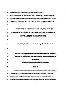
An example of a layered feedforward network is shown in the 3D plot of Fig. 1.2. This kind of network is sometimes also called a multilayer perceptron (MLP) network. Connections only exist between neurons in subsequent layers: subsequent neuron layers are fully interconnected, but connections among neurons within a layer do not exist, nor are there any direct connections across layers. This is the kind of network topology that will be discussed in this thesis, and it can be easily characterized by the number of neurons in each layer, going from input layer (layer 0) to output layer: in Fig. 1.2, the network has a 2-4-4-2 topology7 , where the network inputs are enforced upon the two rectangular input nodes shown at the left side. The actual neural processing elements are denoted by dodecahedrons, such that this particular network contains 10 neurons8 . The network in Fig. 1.2 has two so-called hidden layers, meaning the non-input, non-output layers, i.e., layer 1 and 2. The signals in a feedforward neural network propagate from one network layer to the next. The signal flow is unidirectional: the input to a neuron depends only on the outputs of neurons in the preceding layer, such that no feedback loops exist in the network9 . We will consider the network of Fig. 1.2 to be a 4-layer network, thus including the layer of network inputs in counting layers. There is no general agreement in the literature on whether or not to count the input layer, because it does not compute anything. Therefore, one might prefer to call the network of Fig. 1.2 a 3-layer network. On the other hand, the input layer clearly is a layer, and the number of neural connections to the next layer grows linearly with the number of network inputs, which makes it convenient to consider the input layer as part of the neural network. Therefore one should notice that, although in this thesis the input layer is considered as part of the neural network, a different convention or interpretation will be found in some of the referenced literature. In many cases we will try to circumvent this potential source of confusion by specifying the number of hidden layers of a neural network, instead of specifying the total number of layers. In this thesis, the number of layers in a feedforward neural network is arbitrary, although more than two hidden layers are in practice not often used. The number of neurons in each layer is also arbitrary. The preferred number of layers, as well as the preferred number of 7 Occasionally, we will use a set notation, here for instance giving {2, 4, 4, 2} for the 2-4-4-2 topology, to denote the set of neuron counts for each layer. Using this alternative notation, the “-” separator in the topology specification is avoided, which could otherwise be confused with a minus in cases where the neuron counts are given as symbols or expressions instead of as fixed numerical (integer) values. 8 Here, and elsewhere in this thesis, we do not count the input nodes as (true) neurons, although the input nodes could alternatively also be viewed as dummy neurons with enforced output states. 9 Only during learning, an error signal—derived from the mismatch between the actual network output and the target output—also propagates backward through the network, hence the term “backpropagation learning.” This special kind of “feedback” affects only the regular updating of network parameters, but not the network behaviour for any given (fixed) set of network parameters. The statement about feedback loops in the main text refers to networks with fixed parameters.

10

CHAPTER 1. INTRODUCTION {2, 4, 4, 2}

0 1 2 Layer

3

Figure 1.2: A 2-4-4-2 feedforward neural network example.

neurons in each of the hidden layers, is usually determined via educated guesses and some trial and error on the problem at hand, to find the simplest network that gives acceptable performance. Some researchers create time domain extensions to neural networks via schemes that can be loosely described as being tapped delay lines (the ARMA model used in adaptive filtering also belongs to this class), as in, e.g., [41]. That discrete-time approach essentially concerns ways to evaluate discretized and truncated convolution integrals. In our continuous-time application, we wish to avoid any explicit time discretization in the (finally resulting) model description, because we later want to obtain a description in terms of— continuous-time—differential equations. These differential equations can then be mapped onto equivalent representations that are suitable for use in a circuit simulator, which generally contains sophisticated methods for automatically selecting appropriate time step sizes and integration orders. In other words, we should determine the coefficients of a set of differential equations rather than parameters like delays and tapping weights that have a discrete-time nature or are associated with a particular pre-selected time discretization. In order to determine the coefficients of a set of differential equations, we will in fact need a temporary discretization to make the analysis tractable, but that discretization is not in any way part of the final result, the neural model.

1.4. POTENTIAL ADVANTAGES OF NEURAL MODELLING

1.4

11

Potential Advantages of Neural Modelling

The following list summarizes and discusses some of the potential benefits that may ideally be obtained from the new neural modelling approach—what can be achieved in practice with dynamic neural networks remains to be seen. However, a few of the potential benefits have already been turned into facts, as will be shown in subsequent sections. It should be noted, that the list of potential benefits may be shared, at least in part, by other black-box modelling techniques. • Neural networks could be used to provide a general link from measurements or device simulations to circuit simulation. The discrete set of outcomes of measurements or device simulations can be used as the target data set for a neural network. The neural network then tries to learn the desired behaviour. If this succeeds, the neural network can subsequently be used as a neural behavioural model in a circuit simulator after translating the neural network equations into an appropriate syntax—such as the syntax of the programming language in which the simulator is itself written. One could also use the syntax of the input language of the simulator, as discussed in the next item of this list. An efficient link, via neural network models, between device simulation and circuit simulation allows for the anticipation of consequences of technological choices to circuit performance. This may result in early shifts in device design, processing efforts and circuit design, as it can take place ahead of actual manufacturing capabilities: the device need not (yet) physically exist. Neural network models could then contribute to a reduction of the time-to-market of circuit designs using promising new semiconductor device technologies. Even though the underlying physics cannot be traced within the black-box neural models, the link with physics can still be preserved if the target data is generated by a device simulator, because one can perform additional device simulations to find out how, for instance, diffusion profiles affect the device characteristics. Then one can change the (simulated or real) processing steps accordingly, and have the neural networks adapt to the modified characteristics, after which one can study the effects on circuit-level simulations. • Associated with the neural networks, output drivers can be created for automatically generating models in the appropriate syntax of a set of supported simulators, for example in the form of user models for Pstar or Saber, equivalent electrical circuits for SPICE, or in the form of C code for the Cadence Spectre compiled model interface. Such output drivers will be called model generators. This possibility is discussed in

12

CHAPTER 1. INTRODUCTION more detail in sections 2.5.1, 2.5.2, 4.2.1, 4.2.2.2 and Appendix C. Because a manual implementation of a set of model equations is rather error-prone, the automatic generation of models can help to ensure mutually consistent model implementations for the various supported simulators. Presently, behavioural model generators for Pstar and Berkeley SPICE (and therefore also for the SPICE-compatible Cadence Spectre) already exist. It is a relatively small effort to write other behavioural model generators once the syntax and interfacing aspects of the target simulator are thoroughly understood. As soon as a standard AHDL10 appears, it should be no problem to write a corresponding AHDL model generator. • Neural networks can be generalized to introduce their application to the automatic modelling of device and subcircuit propagation delay effects, manifested in output phase shifts, step responses with ringing effects, opamp slew rates, near-resonant behaviour, etc. This implies the requirement for non-quasistatic (dynamic) modelling, which is a main focus of this thesis. Not only the ever decreasing characteristic feature sizes in VLSI technology cause multidimensional interactions that are hard to analyze physically and mathematically, but also the ever higher frequencies at which these smaller devices are operated cause multidimensional interactions, which in turn lead to major physical and mathematical modelling difficulties. This happens not only at the VLSI level. For instance, parasitic inductances and capacitances due to packaging technology become nonnegligible at very high frequencies. For discrete bipolar devices, this is already a serious problem in practical applications. At some stage, the physical model, even if one can be derived, may become so detailed—i.e., contain so much structural information about the device—that the border between device simulation and circuit simulation becomes blurred, at the expense of simulation efficiency. Although the mathematics becomes more difficult and elaborate when more physical high-frequency interactions are incorporated in the analysis, the actual behaviour of the device or subcircuit does not necessarily become more complicated. Different physical causes may have similar behavioural effects, or partly counteract each other, such that a simple(r) equivalent behavioural model may still exist11 .

10

AHDL = Analogue Hardware Description Language. For example, in deep-submicron semiconductor devices, significant behavioural consequences are caused by the relative dominance of boundary effects. One has to take into account the fact that the electrical fields are non-uniform. This makes a local electrical threshold depend on the position within the device. These multidimensional effects make a thorough mathematical analysis of the overall device behaviour exceedingly difficult. However, the electrical characteristics of the whole device just become simpler in the sense that any “sharp” transitions occurring in the nonlinear behaviour of a large device are now “blurred” by the combined averaging effect of position-dependent internal thresholds. In many 11

1.4. POTENTIAL ADVANTAGES OF NEURAL MODELLING

13

Neural modelling is not hampered by any complicated causes of behaviour: it just concerns the accurate representation of behaviour, in a form that is suitable for its main application area, which in our case is analogue circuit simulation. • Much more compact models, with higher terminal counts, may be obtained than would be possible with table models, because model complexity no longer grows exponentially with the terminal count: the model complexity now typically grows quadratically with the terminal count12 . • Neural networks can in principle automatically detect structures hidden in the target data, and exploit these hidden symmetries or constraints for simplification of the representation, as is done in physical compact modelling. Given a particular neural network, which can be interpreted as a fixed set of computational resources, the (re)allocation of these resources takes place through a learning procedure. Thereby, individual neurons or groups of neurons become dedicated to particular computational tasks that help to obtain an accurate match to the target data. If a hidden symmetry exists, this means that some possible behaviour does not occur, and no neurons will be allocated by a proper learning procedure to non-existent behaviour, because this would not help to improve accuracy. • Neural network models can easily be made infinitely differentiable, as is discussed in section 2.2. This may also be loosely described as making the models infinitely smooth. This is relevant to, for instance, distortion analyses, because discontinuities in higher model derivatives can cause higher harmonics of infinite amplitude, which clearly is unphysical. Model smoothness is also important for the efficiency of the higher order time integration schemes of an analogue circuit simulator. The time integration routines in a circuit simulator typically detect discontinuities of orders that are less than the integration order being used, and respond by temporarily lowering the integration order and/or time step size, which causes significant computational overhead during transient simulations. • Feedforward neural networks can, under relatively mild conditions, be guaranteed to preserve monotonicity in the multidimensional static behaviour. This is shown cases, smooth—at least C 1 —phenomenological models will have less difficulty with the approximation of the resulting more gradual transitions in the device characteristics than they would have had with sharp transitions. 12 To be fair, the exponential growth could still be present in the size of the target data set and in the learning time, because one has to characterize the multidimensional input space of a device or subcircuit. Although this problem can in a number of cases be alleviated by using a priori knowledge about the behaviour, it may in certain cases be a real bottleneck in obtaining an accurate neural model.

14

CHAPTER 1. INTRODUCTION in section 3.3, and subsequently applied to MOSFET modelling in section 4.2.3. With contemporary physical models, it is generally no longer possible to guarantee monotonicity, due to the complexity of the mathematical analysis needed to prove monotonicity. It is an important property, however, because many devices are known to have monotonic characteristics. A nonmonotonic model for such a device may yield multiple spurious solutions for the circuit in which it is applied and it may lead to nonconvergence even during time domain circuit simulation. The monotonicity guarantee for neural networks can be maintained for highly nonlinear multidimensional behaviour, which so far has not been possible with table models without requiring excessive amounts of data [39]. Furthermore, the monotonicity guarantee is optional, such that nonmonotonic static behaviour can still be modelled, as is illustrated in section 4.2.1. • Stability13 of feedforward neural networks can be guaranteed. The stability of feedforward neural networks depends solely on the stability of its individual neurons. If all neurons are stable, then the feedforward network is also stable. Stability of individual neurons is ensured through parameter constraints imposed upon their associated differential equations, as shown in sections 2.3.2 and 4.1.2. • Feedforward neural networks can be defined in such a way that it can be guaranteed that the networks each have a unique behaviour for a given set of (time-dependent) inputs. This implies, as is shown in section 3.1.1.1, that the corresponding neural models have unique solutions in both dc and transient analysis when they are applied in circuit simulation. This property can help the nonlinear solver of a circuit simulator to converge and it also helps to avoid spurious solutions to circuit behaviour. On the other hand, it is at the same time a limitation to the modelling capabilities of these neural networks, for there may be situations in which one wants to model the multiple solutions in the behaviour of a resistive device or subcircuit, for example when modelling a flip-flop. So it must be a deliberate choice, made to help with the modelling of a restricted class of devices and subcircuits. In this thesis, the uniqueness restriction is accepted in order to make use of the associated desirable mathematical and numerical properties. • Feedforward neural networks can be defined in such a way, that the static behaviour of a network, i.e., the dc solution, can be obtained from nonlinear but explicit formu-

13

Stability here refers to the system property that for times going towards infinity, and for constant inputs to the system under consideration, and for any starting condition, the system moves into a static equilibrium state, which is also called a stable focus [10].

1.5. OVERVIEW OF THE THESIS

15

las, thereby avoiding the need for an iterative solver for implicit nonlinear equations. Therefore, convergence problems cannot occur during the dc analysis of neural networks with enforced inputs14 . Simulation times are in general also significantly reduced by avoiding the need for iterative nonlinear solvers. • The learning procedures for neural networks can be made flexible enough to allow the grid-free specification of multidimensional input data. This makes the adaptation and use of existing measurement or device simulation data formats much easier. The proper internal coordinate system is in principle discovered automatically, instead of being specified by the user (as is required for table models)15 . • Neural networks may also find applications in the macromodelling of analogue nonlinear dynamic systems, e.g., subcircuits and standard cells. Resulting behavioural models may replace subcircuits in simulations that would otherwise be too timeconsuming to perform with an analogue circuit simulator like Pstar. This could effectively result in a form of mixed-level simulation with preservation of loading effects and delays, without requiring the tight integration of two or more distinct simulators.

1.5

Overview of the Thesis

The general heading of this thesis is to first define a class of dynamic neural networks, then to derive a theory and algorithms for training these neural networks, subsequently to implement the theory and algorithms in software, and then to apply the software to a number of test-cases. Of course, this idealized logical structure does not quite reflect the way the work is done, in view of the complexity of the subject. In reality one has to consider, as early as possible, aspects from all these stages at the same time, in order to increase the probability of obtaining a practical compromise between the many conflicting requirements. Moreover, insights gained from software experiments may in a sense “backpropagate” and lead to changes even in the neural network definitions. 14

This will hold for our neural network simulation and optimization software, which makes use of expressions like those given in section 3.1.1.1, Eq. (3.6). If behavioural models are generated for another simulator, it still depends upon the algorithms of this other simulator whether convergence problems can occur: it might try to solve an explicit formula implicitly, since we cannot force another simulator to be “smart.” Furthermore, if some form of feedback is added to the neural networks, the problems associated with nonlinear implicit equations generally return, because the values of network input variables involved in the feedback will have to be solved from nonlinear implicit equations. 15 An exception still remains when guarantees for monotonicity are required. Monotonicity at all points and in each of the coordinate directions of one selected coordinate system, does not imply monotonicity in each of the directions of another coordinate system. Monotonicity is therefore in principle coupled to the particular choice of a coordinate system, as will be briefly discussed later on, in section 3.3, for a bipolar modelling example.

16

CHAPTER 1. INTRODUCTION

In chapter 2, the equations for dynamic feedforward neural networks are defined and discussed. The behaviour of individual neurons is analyzed in detail. In addition, the representational capabilities of these networks are considered, as well as some possibilities to construct equivalent electrical circuits for neurons, thereby allowing their direct application in analogue circuit simulators. Chapter 3 shows how the definitions of chapter 2 can be used to construct sensitivitybased learning procedures for dynamic feedforward neural networks. The chapter has two major parts, consisting of sections 3.1 and 3.2. Section 3.1 considers a representation in the time domain, in which neural networks may have to learn step responses or other transient responses. Section 3.2 shows how the definitions of chapter 2 can also be employed in a small-signal frequency domain representation, by deriving a corresponding sensitivity-based learning approach for the frequency domain. Time domain learning can subsequently be combined with frequency domain learning. As a special topic, section 3.3 discusses how monotonicity of the static response of feedforward neural networks can be guaranteed via parameter constraints during learning. The monotonicity property is particularly important for the development of suitable device models for use in analogue circuit simulators. Chapter 4, section 4.1, discusses several aspects concerning an experimental software implementation of the time domain learning and frequency domain learning techniques of the preceding chapter. Section 4.2 then shows a number of preliminary modelling results obtained with this experimental software implementation. The neural modelling examples involve time domain learning and frequency domain learning, and use is made of the possibility to automatically generate analogue behavioural (macro)models for circuit simulators. Finally, chapter 5 draws some general conclusions and sketches recommended directions for further research.

Chapter 2

Dynamic Neural Networks In this chapter, we will define and motivate the equations for dynamic feedforward neural networks. The dynamical properties of individual neurons are analyzed in detail, and conditions are derived that guarantee stability of the dynamic feedforward neural networks. Subsequently, the ability of the resulting networks to represent various general classes of behaviour is discussed. The other way around, it is shown how the dynamic feedforward neural networks can themselves be represented by equivalent electrical circuits, which enables the use of neural models in existing analogue circuit simulators. The chapter ends with some considerations on modelling limitations.

2.1

Introduction to Dynamic Feedforward Neural Networks

Dynamic feedforward neural networks are conceived as mathematical constructions, independent of any particular physical representation or interpretation. This section shows how these artificial neural networks can be related to device and subcircuit models that involve physical quantities like currents and voltages.

2.1.1

Electrical Behaviour and Dynamic Feedforward Neural Networks

In general, an electronic circuit consisting of arbitrarily controlled elements can be mathematically described by a system of nonlinear first order differential equations1 f (x(t) ,

dx(t) ,p ) = 0 dt

(2.1)

1 Actually, we may have a system of differential algebraic equations (DAE’s), characterized by the fact that not all equations are required to contain differential terms. However, one can also view such an algebraic equation as a special case of a differential equation, involving differential terms that are multiplied by zero-valued coefficients. Therefore, we will drop the adjective “algebraic” for brevity.

17

18

CHAPTER 2. DYNAMIC NEURAL NETWORKS

with f a vector function. The real-valued2 vector x can represent any mixture of electrical input variables, internal variables and output variables at times t. An electrical variable can be a voltage, a current, a charge or a flux. The real-valued vector p contains all the circuit and device parameters. Parameters may represent component values for resistors, inductors and capacitors, or the width and length of MOSFETs, or any other quantities that are fixed by the particular choice of circuit design and manufacturing process, but that may, at least in principle, be adapted to optimize circuit or device performance. Constants of nature, such as the speed of light or the Boltzmann constant, are therefore not considered as parameters. It should perhaps be explicitly stated, that in this thesis a parameter is always considered to be constant, except for a possible regular updating as part of an optimization procedure that attempts to obtain a desired behaviour for the variables of a system by searching for a suitable set of parameter values. For practical reasons, such as the crucial model simplicity (to keep the model evaluation times within practical bounds), and to be able to give under certain conditions guarantees on some desirable properties (uniqueness of solution, monotonicity, stability, etc.), we will move away from the general form of Eq. (2.1), and restrict the dependencies to those of layered feedforward neural networks, excluding interactions among different neurons within the same layer. Two subsequent layers are fully interconnected. The feedforward approach allows the definition of nonlinear networks that do not require an iterative method for solving state variables from sets of nonlinear equations (contrary to the situation with most nonlinear electronic circuits), and the existence of a unique solution of network state variables for a given set of network inputs can be guaranteed. As is conventional for feedforward networks, neurons receive their input only from outputs in the layer immediately preceding the layer in which they reside. A net input to a neuron is constructed as a weighted sum, including an offset, of values obtained from the preceding layer, and a nonlinear function is applied to this net input. However, instead of using only a nonlinear function of a net input, each neuron will now also involve a linear differential equation with two internal state variables, driven by a nonlinear function of the net input, while the net input itself will include time derivatives of outputs from the preceding layer. This enables each single neuron, in concert with its input connections, to represent a second order band-pass type filter, which makes even individual neurons very powerful building blocks for modelling. Together these neurons constitute a dynamic feedforward neural network, in which each neuron still receives input only from the preceding layer. In our new neural network modelling approach, dynamic 2 In the remainder of this thesis, it will very often not be explicitly specified whether a variable, parameter or function is real-valued, complex-valued or integer-valued. This omission is mainly for reasons of readability. The appropriate value type should generally be apparent from the context, application area, or conventional use in the literature.

2.1. INTRODUCTION TO DYNAMIC FEEDFORWARD NEURAL NETWORKS

19

semiconductor device and subcircuit behaviour is to be modelled by this kind of neural network. The design of neurons as powerful building blocks for modelling implies that we deliberately support the grandmother-cell concept3 in these networks, rather than strive for a distributed knowledge representation for (hardware) fault-tolerance. Since fault-tolerance is not (yet) an issue in software-implemented neural networks, this is not considered a disadvantage for our envisioned software applications.

2.1.2

Device and Subcircuit Models with Embedded Neural Networks

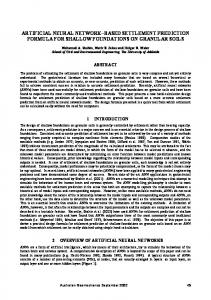
The most common modelling situation is that the terminal currents of an electrical device or subcircuit are represented by the outcomes of a model that receives a set of independent voltages as its inputs. This also forms the basis for one of the most prevalent approaches to circuit simulation: Modified Nodal Analysis (MNA) [10]. Less common situations, such as current-controlled models, can still be dealt with, but they are usually treated as exceptions. Although our neural networks do not pertain to any particular choice of physical quantities, we will generally assume that a voltage-controlled model for the terminal currents is required when trying to represent an electronic device or subcircuit by a neural model. A notable exception is the representation of combinatorial logic, where the relevant inputs and outputs are often chosen to be voltages on the subcircuit terminals in two disjoint sets: one set of terminals for the inputs, and another one for the outputs. This choice is in fact less general, because it neglects loading effects like those related to fan-in and fan-out. However, the representation of combinatorial logic is not further pursued in this thesis, because our main focus is on learning truly analogue behaviour rather than on constructing analogue representations of essentially digital behaviour4 . The independent voltages of a voltage-controlled model for terminal currents may be defined w.r.t. some reference terminal. This is illustrated in Fig. 2.1, where n voltages w.r.t. a reference terminal REF form the inputs for an embedded dynamic feedforward neural network. The outputs of the neural network are interpreted as terminal currents, and the neural network outputs are therefore assigned to corresponding controlled current 3

In the neural network literature, this refers to the situation that a single neuron performs a specific “task”—such as recognizing one’s grandmother. Removal of this neuron makes the neural network fail on this task. In a so-called distributed representation, however, the removal of any single neuron will have little effect on the performance of the neural network on any of its tasks. 4 The design of constructive, i.e., learning-free, procedures that map for instance a logic sp-form [6, 31] onto a corresponding topology and parameter set of an equivalent feedforward neural network is certainly possible, including a rough representation of propagation delay, but a full description would require a rather extensive introduction to the terminology of logic synthesis. That in turn would shift the emphasis of this thesis too much away from the time domain and frequency domain learning techniques.

20

CHAPTER 2. DYNAMIC NEURAL NETWORKS

sources of the model for the electrical behaviour of an (n+1)-terminal device or subcircuit. Only n currents need to be explicitly modelled, because the current through the single remaining (reference) terminal follows from the Kirchhoff current law as the negative sum of the n explicitly modelled currents. At first glance, Fig. 2.1 may seem to represent a system with feedback. However, this is not really the case, since the information returned to the terminals concerns a physical quantity (current) that is entirely distinct from the physical quantity used as input (voltage). The input-output relation of different physical quantities may be associated with the same set of physical device or subcircuit terminals, but this should not be confused with feedback situations where outputs affect the inputs because they refer to, or are converted into, the same physical quantities. In the case of Fig. 2.1, the external voltages may be set irrespective of the terminal currents that result from them. In spite of the reduced model (evaluation) complexity, the mathematical notations in the following sections can sometimes become slightly more complicated than needed for a general network description, due to the incorporation of the topological restrictions of feedforward networks in the various derivations.

Figure 2.1: A dynamic feedforward neural network embedded in a voltage-controlled device or subcircuit model for terminal currents.

2.2. DYNAMIC FEEDFORWARD NEURAL NETWORK EQUATIONS

2.2 2.2.1

21

Dynamic Feedforward Neural Network Equations Notational Conventions

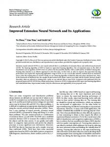
Before one can write down the equations for dynamic feedforward neural networks, one has to choose a set of labels or symbols with which to denote the various components, parameters and variables of such networks. The notations in this thesis closely follow and extend the notations conventionally used in the literature on static feedforward neural networks. This will facilitate reading and make the dynamic extensions more apparent for those who are already familiar with the latter kind of networks. The illustration of Fig. 2.2 can be helpful in keeping track of the relation between the notations and the neural network components. The precise purpose of some of the notations will only become clear in subsequent sections. A feedforward neural network will be characterized by the number of layers and the number of neurons per layer. Layers are counted starting with the input layer as layer 0, such that a network with output layer K involves a total of K + 1 layers (which would have been K layers in case one prefers not to count the input layer). Layer k by definition contains Nk neurons, where k = 0, · · · , K. The number Nk may also be referred to as the width of layer k. Neurons that are not directly connected to the inputs or outputs of the network belong to a so-called hidden layer, of which there are K − 1 in a (K + 1)-layer network. (0)

Network inputs are labeled as x(0) ≡ (x1

(0)

, · · · , xN0 )T , and network outputs as x(K) ≡

Figure 2.2: Some notations associated with a dynamic feedforward neural network.

22 (K)

(x1

CHAPTER 2. DYNAMIC NEURAL NETWORKS (K)

, · · · , xNK )T .

The neuron output vector y k ≡ (y1,k , · · · , yNk ,k )T represents the vector of neuron outputs for layer k, containing as its elements the output variable yi,k for each individual neuron i in layer k. The network inputs will be treated by a dummy neuron layer k = 0, with (0)

enforced neuron j outputs yj,0 ≡ xj , j = 0, · · · , N0 . This sometimes helps to simplify the notations used in the formalism. However, when counting the number of neurons in a network, we will not take the dummy input neurons into account. We will apply the convention that separating commas in subscripts are usually left out if this does not cause confusion. For example, a weight parameter wi,j,k may be written as wijk , which represents a weighting factor for the connection from5 neuron j in layer k − 1 to neuron i in layer k. Separating commas are normally required with numerical values for subscripts, in order to distinguish, for example, w12,1,3 from w1,21,3 and w1,2,13 — unless, of course, one has advance knowledge about topological restrictions that exclude the alternative interpretations. A weight parameter wijk sets the static connection strength for connecting neuron j in layer k − 1 with neuron i in layer k, by multiplying the output yj,k−1 by the value of wijk . An additional weight parameter vijk will play the same role for the frequency dependent part of the connection strength, which is an extension w.r.t. static neural networks. It is a weighting factor for the rate of change in the output of neuron j in layer k − 1, multiplying the time derivative dyj,k−1 /dt by the value of vijk . In view of the direct association of the extra weight parameter vijk with dynamic behaviour, it is also considered to be a timing parameter. Depending on the context of the discussion, it will therefore be referred to as either a weight(ing) parameter or a timing parameter. As the notation already suggests, the parameters wijk and vijk are considered to belong to neuron i in layer k, which is analogous to the fact that much of the weighted input processing of a biological neuron is performed through its own branched dendrites. The vector of weight parameters wik ≡ (wi,1,k , · · · , wi,Nk−1 ,k )T is conventionally used to determine the orientation of a static hyperplane, by setting the latter orthogonal to wik . A threshold parameter θik of neuron i in layer k is then used to determine the position, or offset, of this hyperplane w.r.t. the origin. Separating hyperplanes as given by wik ·y k−1 −θik = 0 are known to form the backbone for the ability to represent arbitrary static classifications in discrete problems [36], for example occurring with combinatorial logic, and they can play a similar role in making smooth transitions among (qualitatively) 5 This differs only slightly from the convention in the neural network literature, where a weight wij usually represents a connection from a neuron j to a neuron i in some layer. Not specifying which layer is often a cause of confusion, especially in textbooks that attempt to explain backpropagation theory, because one then tries to put into words what would have been far more obvious from a well-chosen notation.

2.2. DYNAMIC FEEDFORWARD NEURAL NETWORK EQUATIONS

23

different operating regions in analogue applications. The (generally) nonlinear nature of a neuron will be represented by means of a (generally) nonlinear function F, which will normally be assumed to be the same function for all neurons within the network. However, when needed, this is most easily generalized to different functions for different neurons and different layers, by replacing any occurrence of F by F (ik) in every formula in the remainder of this thesis, because in the mathematical derivations the F always concerns the nonlinearity of one particular neuron i in layer k: it always appears in conjunction with an argument sik that is unique to neuron i in layer k. For these reasons, it seemed inappropriate to further complicate, or even clutter, the already rather complicated expressions by using neuron-specific superscripts for F. However, it is useful to know that a purely linear output layer can be created6 , since that is the assumption underlying a number of theorems on the representational capabilities of feedforward neural networks having a single hidden layer [19, 23, 34]. The function F is for neuron i in layer k applied to a weighted sum sik of neuron outputs yj,k−1 in the preceding layer k − 1. The weighting parameters wijk , vijk and threshold parameter θik take part in the calculation of this weighted sum. Within a nonlinear function F for neuron i in layer k, there may be an additional (transition) parameter δik , which may be used to set an appropriate scale of change in qualitative transitions in function behaviour, as is common to semiconductor device modelling7 . Thus the application of F for neuron i in layer k takes the form F(sik , δik ), which reduces to F(sik ) for functions that do not depend on δik . The dynamic response of neuron i in layer k is determined not only by the timing parameters vijk , but also by additional timing parameters τ1,ik and τ2,ik . Whereas the contributions from vijk amplify rapid changes in neural signals, the τ1,ik and τ2,ik will have the opposite effect of making the neural response more gradual, or time-averaged. In order to guarantee that the values of τ1,ik and τ2,ik will always lie within a certain desired range, they may themselves be determined from associated parameter functions8 τ1,ik = τ1 (σ1,ik , σ2,ik ) and τ2,ik = τ2 (σ1,ik , σ2,ik ). These functions will be constructed in such a way that no constraints on the (real) values of the underlying timing parameters σ1,ik and σ2,ik are needed to obtain appropriate values for τ1,ik and τ2,ik .

6 Linearity in an output layer with nonlinear neurons can on a finite argument range also be approximated up any desired accuracy by appropriate scalings of weights and thresholds, but that procedure is less direct, and it is restricted to mappings with a finite range. The latter restriction will normally not be a practical problem in modelling physical systems. 7 In principle, one could extend this to the use of a parameter vector δ ik , but so far a single scalar δik appeared sufficient for our applications. 8 The detailed reasons for introducing these parameter functions are explained further on.

24

2.2.2

CHAPTER 2. DYNAMIC NEURAL NETWORKS

Neural Network Differential Equations and Output Scaling

The differential equation for the output, or excitation, yik of one particular neuron i in layer k > 0 is given by

τ2 (σ1,ik , σ2,ik )

d2 yik dyik + τ1 (σ1,ik , σ2,ik ) + yik = F(sik , δik ) 2 dt dt

(2.2)

with the weighted sum s of outputs from the preceding layer

4

sik = wik · y k−1 − θik + v ik ·

dy k−1 dt

Nk−1

=

X

Nk−1

wijk yj,k−1 − θik +

j=1

X

vijk

j=1

dyj,k−1 dt

(2.3)

for k > 1, and similarly for the neuron layer k = 1 connected to the network input

4

sik = wik · x(0) − θik + v ik · =

N0 X

(0) wij,0 xj

− θi,0 +

j=1

dx(0) dt N0 X j=1

(0)

vij,0

dxj dt

(2.4)

which, as stated before, is entirely analogous to having a dummy neuron layer k = 0 with (0)

enforced neuron j outputs yj,0 ≡ xj . In the following, we will occasionally make use of this in order to avoid each time having to make notational exceptions for the neuron layer k = 1, and we will at times refer to Eq. (2.3) even for k = 1. The net input sik is analogous to the weighted input signal arriving at the cell body, or soma, of a biological neuron via its branched dendrites, where its value determines whether or not the neuron will fire a signal through its output, the axon, and at what spike rate. Eq. (2.2) can therefore be viewed as the mathematical description of the neuron cell body. In our formalism, we have no analogue of a branched axon, because the branching of the inputs is sufficiently general for the feedforward network topology that we use9 . 9 One could alternatively view the set of weights, directed to a given layer and coming from one particular neuron in the preceding layer, as a branched axon for the output of that particular neuron. Then we would no longer need the equivalent of dendrites, and we could relabel the weights as belonging to neurons in the preceding layer. All this would not make any difference to the network functionality: it merely concerns

2.2. DYNAMIC FEEDFORWARD NEURAL NETWORK EQUATIONS

25

Finally, to allow for arbitrary network output ranges—because, normally, nonlinear functions F are used that squash the steady state neuron inputs into a finite output range, such as [0, 1] or [−1, 1]—the time-dependent outputs yiK of neurons i in the output layer (K)

K yield the network output excitations xi

(K)

xi

through a linear scaling transformation

= αi yiK + βi

(2.5)

yielding a network output vector x(K) . There is no fundamental reason why a learning scheme would not yield inappropriate values for the coefficients of the differential terms in a differential equation, which could lead to unstable or resonant behaviour, or give rise to still other undesirable kinds of behaviour. Even if this occurs only during the learning procedure, it may at least slow down the convergence towards a “reasonable” behaviour, whatever we may mean by that, but it may also enhance the probability of finding an inappropriate local minimum. To decrease the probability of such problems, a robust software implementation may actually 4

4

employ functions like τ1,ik = τ1 (σ1,ik , σ2,ik ) and τ2,ik = τ2 (σ1,ik , σ2,ik ) that have any of the relevant—generally nonlinear—constraints built into the expressions. As a simple 2 2 , and the neural network tries to learn the example, if τ1,ik = σ1,ik and τ2,ik = σ2,ik

underlying parameters σ1,ik and σ2,ik , then it is automatically guaranteed that τ1,ik and τ2,ik are not negative. More sophisticated schemes are required in practice, as will be discussed in section 4.1.2. In the following, the parameter functions τ1 (σ1,ik , σ2,ik ) and τ2 (σ1,ik , σ2,ik ) are often simply denoted by (timing) “parameters” τ1,ik and τ2,ik , but it must be kept in mind that these are only indirectly, namely via the σ’s, determined in a learning scheme. Finally, it should be noted that the τ1,ik have the dimension of time, but the τ2,ik have the dimension of time squared.

2.2.3

Motivation for Neural Network Differential Equations

The selection of a proper set of equations for dynamic neural networks cannot be performed through a rigid procedure. Several good choices may exist. The final selection made for this thesis reflects a mixture of—partly heuristic—considerations on desirable properties and “circumstantial evidence” (more or less in hindsight) for having made a good choice. Therefore, we will in the following elaborate on some of the additional reasons that led to the choice of Eqs. (2.2) and (2.3): the way we wish to denote and distinguish for ourselves the different components of a neural network.

26

CHAPTER 2. DYNAMIC NEURAL NETWORKS • A nonlinear, typically sigmoid10 , function F with at least two identifiable operating regions provides a general capability for representing or approximating arbitrary discrete (static) classifications—even for disjoint sets—using a static (dc) feedforward network and requiring not more than two hidden layers [36]. • A nonlinear, monotonically increasing and bounded continuous function F also provides a general capability for representing any continuous multidimensional (multivariate) static behaviour up to any desired accuracy, using a static feedforward network and requiring not more than one hidden layer [19, 23]. Recently, it has even been shown that F need only be nonpolynomial in order to prove these representational capabilities [34]. More literature on the capabilities of neural networks and fuzzy systems as universal static approximators can be found in [4, 7, 24, 26, 27, 33]. • It will be shown by construction in section 2.4.1, that this ability to represent any multidimensional static behaviour almost trivially extends to arbitrary quasistatic behaviour, when using Eqs. (2.2), (2.3) and (2.5), while requiring no more than two hidden layers. • The use of an infinitely differentiable, i.e., C ∞ , function F makes the whole neural network infinitely differentiable. This is relevant to the accuracy of neural network models in distortion analyses, but it is also important for the efficiency of the higher order time integration schemes of an analogue circuit simulator in which the neural network models will be incorporated. • A single neuron can already exactly represent the dynamic behaviour of elementary but fundamental linear electronic circuits like a voltage-driven (unloaded) RC-stage, or an output-grounded RCR-stage from a ladder network. The heuristic but pragmatic guideline here is that simple electronic circuits should be representable by few neurons. If not, it would become doubtful whether more complicated electronic circuits could be represented efficiently. • The term with vijk provides the capability for time-differentiation of input signals to the neuron, thereby amplifying, or “detecting,” rapid changes in the neuron input signals. • The terms with wijk and vijk together provide the capability to represent, in a very natural way, the full complex-valued admittance matrices arising in low-frequency quasistatic modelling. This ensures that low-frequency modelling nicely fits the mathematical structure of the neural network, which will generally speed up learning

10

A sigmoid function is defined as being a strictly increasing differentiable function with a finite range.

2.2. DYNAMIC FEEDFORWARD NEURAL NETWORK EQUATIONS

27

progress. In electrical engineering, an admittance matrix Y is often written as Y = G + ωC, where G is a real-valued conductance matrix and C a real-valued capacitance matrix. The dot-less symbol  is in this thesis used to denote the complex constant fulfilling 2 = −1. The (angular) frequency is denoted by ω, and the factor ω then corresponds to time differentiation. Since the number of elements in a (square) matrix grows quadratically with the size of the matrix, we need a structure of comparable complexity in a neural network. Only the weight components wijk and vijk meet this growth in complexity: the wijk can play the role of the conductance matrix elements (G)ij , while the vijk can do the same for the capacitance matrix elements (C)ij

11 .

• A further reason for the combination of wijk and vijk lies in the fact that it simplifies the representation of diffusion charges of forward-biased bipolar junctions, in which the dominant charges are roughly proportional to the dc currents, which themselves depend on the applied voltage bias in a strongly nonlinear (exponential) fashion. The total current, consisting of the dc current and the time derivative of the diffusion charge, is then obtained by first calculating a bias-dependent nonlinear function having a value proportional to the dc current. In a subsequent neural network layer, this function is weighted by wijk to add the dc current to the net input of a neuron, and its time derivative is weighted by vijk to add the capacitive current to the net input. The resulting total current is transparently copied to the network output through appropriate parameter settings that linearize the behaviour of the output neurons. This whole procedure is very similar to the constructive procedure, given in section 2.4.1, to demonstrate that arbitrary quasistatic models can be represented by our generalized neural networks. • The term with τ1,ik provides the capability for time-integration to the neuron, thereby also time-averaging the net input signal sik . For τ2,ik = 0 and vijk = 0, this is the same kind of low-pass filtering that a simple linear circuit consisting of a resistor in series with a capacitor performs, when driven by a voltage source. • The term with τ2,ik suppresses the terms with vijk for very high frequencies. This ensures that the neuron (and neural network) transfer will drop to zero for sufficiently high frequencies, as happens with virtually any physical system. • If all the τ1,ik and τ2,ik in a neural network are constrained to fulfill τ1,ik > 0 and τ2,ik > 0, then this neural network is guaranteed to be stable in the sense that the time-varying parts of the neural network outputs vanish for constant network inputs 11

In linear modelling, this applies to a 2-layer linear neural model with voltage inputs and current outputs, using F(sik ) ≡ sik , τ1,ik = τ2,ik = 0 and αi = 1. The θik and βi relate to arbitrary offsets.

28

CHAPTER 2. DYNAMIC NEURAL NETWORKS and for times going towards infinity. This topic will be covered in more detail in section 2.3.2. • Further on, in section 3.1.1.1, we will also show that the choice of Eqs. (2.2) and (2.3) avoids the need for a nonlinear solver during dc and transient analysis of the neural networks. Thereby, convergence problems w.r.t. the dynamic behaviour of the neural networks simply do not exist, while the efficiency is greatly improved by always having just one “iteration” per time step. These are major advantages over general circuit simulation of arbitrary systems having internal nodes for which the behaviour is governed by implicit nonlinear equations.

The complete neuron description from Eqs. (2.2) and (2.3) can act as a (nonlinear) band-pass filter for appropriate parameter settings: the amplitude of the vijk -terms will grow with frequency and dominate the wijk - and θik -terms for sufficiently high frequencies. However, the τ1,ik -term also grows with frequency, leading to a transfer function amplitude on the order of vijk /τ1,ik , until τ2,ik comes into play and gradually reduces the neuron highfrequency transfer to zero. A band-pass filter approximates the typical behaviour of many physical systems, and is therefore an important building block in system modelling. The non-instantaneous response of a neuron is a consequence of the terms with τ1,ik and τ2,ik .

2.2.4

Specific Choices for the Neuron Nonlinearity F

If all timing parameters in Eqs. (2.2) and (2.3) are zero, i.e., vijk = τ1,ik = τ2,ik = 0, and if one applies the familiar logistic function L(sik )

4

4

F0 (sik ) = L(sik ) =

1 −s 1 + e ik

(2.6)

then one obtains the standard static (not even quasi-static) networks often used with the popular error backpropagation method, also known as the generalized delta rule, for feedforward neural networks. Such networks are therefore special cases of our dynamic feedforward neural networks. The logistic function L(sik ), as illustrated in Fig. 2.3, is strictly monotonically increasing in sik . However, we will generally use nonzero v’s and τ ’s, and will instead of the logistic function apply other infinitely smooth (C ∞ ) nonlinear modelling functions F. The standard logistic function lacks the common transition between highly nonlinear and weakly nonlinear behaviour that is typical for semiconductor devices and circuits12 . 12

One may think of simple examples like the transition in MOSFET drain currents when going from

2.2. DYNAMIC FEEDFORWARD NEURAL NETWORK EQUATIONS

29

F0 1

0.8

0.6

0.4

0.2

-5

-10

5

10

s

Figure 2.3: Logistic function L(sik ).

One of the alternative functions for semiconductor device modelling is

4

F1 (sik , δik ) = =

1 δik

sik + δik ln cosh 2 s + δ cosh ik 2 ik 1 ln δik δik cosh sik − 2 





sik − δik − ln cosh 2 



(2.7)

with δik 6= 0. This sigmoid function is strictly monotonically increasing in the variable sik , and even antisymmetric in sik : F1 (sik , δik ) = −F1 (−sik , δik ), as illustrated in Fig. 2.4. Note, however, that the function is symmetric13 in δik : F1 (sik , δik ) = F1 (sik , −δik ). For |δik |  0, Eq. (2.7) behaves asymptotically as F1 (sik , δik ) ≈ −1 + exp(sik + δik )/|δik | for sik < −|δik |, F1 (sik , δik ) ≈ sik /|δik | for −|δik | < sik < |δik |, and F1 (sik , δik ) ≈ 1 − exp(δik − sik )/|δik | for sik > |δik |. The function defined in Eq. (2.7) needs to be subthreshold to strong inversion by varying the gate potential, or of the current through a series connection of a resistor and a diode, when driven by a varying voltage source. When evaluating L(wijk yj,k−1 ) for large positive values of wijk , one indeed obtains highly nonlinear exponential “diode-like” behaviour as a function of yj,k−1 for yj,k−1  0 or yj,k−1  0 (not counting a fixed offset of size 1 in the latter case). However, at the same time one obtains an undesirable very steep transition around yj,k−1 = 0, approaching a discontinuity for wijk → ∞. 13 Symmetry of a non-constant function implies nonmonotonicity. However, monotonicity in parameter space is usually not required, because it does not cause problems in circuit simulation, where only the dc monotonicity in (electrical) variables counts.

30

CHAPTER 2. DYNAMIC NEURAL NETWORKS

rewritten into several numerically very different but mathematically equivalent forms for improved numerical robustness, to avoid loss of digits, and for computational efficiency in the actual implementation. The function is related to the logistic function in the sense that it is, apart from a linear scaling, the integral over sik of the difference of two transformed logistic functions, obtained by shifting one logistic function by −δik along the sik -axis, and another logistic function by +δik . This construction effectively provides us with a polynomial (linear) region and two exponential saturation regions. Thereby we have the practical equivalent of two typically dominant basis functions for semiconductor device modelling, the motivation for which runs along similar lines of thought as in highly nonlinear multidimensional table modelling [39]. To show the integral relation between L and F1 , we first note that the logistic function L is related to the tanh function by

2L(x) − 1 =

2

−1 = 1 + e −x

e e

+x/2 +x/2

−e +e

−x/2 −x/2

= tanh

x 2

(2.8)

The indefinite integral of the tanh(x) function is ln(cosh(x)) (neglecting the integration constant), as is readily verified by differentiating the latter, and we easily obtain

Z

x x + ln cosh 2 2 

L(x) dx =



(2.9)

1 0.5 0 F1 -0.5 -1 10

10 0

0 delta

-10

Figure 2.4: Neuron nonlinearity F1 (sik , δik ).

-10

s

2.2. DYNAMIC FEEDFORWARD NEURAL NETWORK EQUATIONS

31

such that we find, using the symmetry of the cosh function, 1 δik

Z sik

0

(L(x + δik ) − L(x − δik )) dx =

1 x + δik + ln cosh x + δik − x − δik + ln cosh x − δik 2 2 2 2 δik  sik x + δik sik + δik 1 ln cosh 1 ln cosh 2  2 = δik δ x − δ s − δik ik ik ik cosh cosh 2 2 0 h









isik

0

=

(2.10)

which is the F1 (sik , δik ) defined in Eq. (2.7). Another interesting property is that the F1 (sik , δik ) reduces again to a linearly scaled logistic function for δik approaching zero, i.e., sik lim F1 (sik , δik ) = 2L(sik ) − 1 = tanh δik →0 2 



(2.11)

The limit is easily obtained by linearizing the integrand in the first line of Eq. (2.10) at x as a function of δik , or alternatively by applying l’Hˆopital’s rule. Derivatives of F1 (sik , δik ) in Eq. (2.7) are needed for transient sensitivity (first partial derivatives only) and for ac sensitivity (second partial derivatives for dc shift), and are given by ∂F1 1 = (L(sik + δik ) − L(sik − δik )) ∂sik δik

(2.12)

1 ∂ 2 F1 = (L(sik + δik )[1 − L(sik + δik )] − L(sik − δik )[1 − L(sik − δik )]) δik ∂s2ik

(2.13)

∂F1 1 = (L(sik + δik ) + L(sik − δik ) − F1 (sik , δik ) − 1) ∂δik δik

(2.14)

∂ 2 F1 ≡ ∂ 2 F1 = ∂δik ∂sik ∂sik ∂δik   1 L(s + δ )[1 − L(s + δ )] + L(s − δ )[1 − L(s − δ )] − ∂F1 ik ik ik ik ik ik ik ik δik ∂sik

(2.15)

The strict monotonicity of F1 is obvious from the expression for the first partial derivative in Eq. (2.12), since, for positive δik , the first term between the outer parentheses is always larger than the second term, in view of the fact that L is strictly monotonically increasing. For negative δik , the second term is the largest, but the sign change of the factor 1/δik compensates the sign change in the subtraction of terms between parentheses, such that the first partial derivative of F1 w.r.t. sik is always positive for δik 6= 0.

32

CHAPTER 2. DYNAMIC NEURAL NETWORKS

Yet another choice for F uses the argument δik only to control the sharpness of the transition between linear and exponential behaviour, without simultaneously varying the size of the near-linear interval. Preliminary experience with modelling MOSFET dc characteristics indicates that this helps to avoid unacceptable local minima in the error function (cost function) for optimization—unacceptable in the sense that the results show too gradual near-subthreshold transitions. Another choice for F(sik , δik ) is therefore defined as

4

F2 (sik , δik ) =

=

1 2 δik

"

δ 2 (sik + 1) ln cosh ik 2

!

δ 2 (sik − 1) − ln cosh ik 2

δ 2 (s + 1) cosh ik ik 1 2 2 ln 2 (s − 1) δik δik ik cosh 2

!#

(2.16)

1 0.5 0 F2 -0.5 -1 5

2 2.5 0

0 -2.5 delta

-5

-2

s

Figure 2.5: Neuron nonlinearity F2 (sik , δik ).

where the square of δik 6= 0 avoids the need for absolute signs, while it also keeps practical values of δik for MOSFET subthreshold and bipolar modelling closer to 1, i.e., nearer to typical values for most other parameters in a suitably scaled neural network (see also 2 ≈ 40 would be typical for Boltzmann factors. The section 4.1.1). For instance, δik

properties of F2 are very similar to those of F1 , since it is actually a differently scaled

2.3. ANALYSIS OF NEURAL NETWORK DIFFERENTIAL EQUATIONS

33

version of F1 : 2 2 F2 (sik , δik ) ≡ F1 (δik sik , δik )

(2.17)

So the antisymmetry (in s) and symmetry (in δ) properties still hold for F2 . For |δik |  0, 2 (s + 1))/δ 2 for s < −1, Eq. (2.16) behaves asymptotically as F2 (sik , δik ) ≈ −1 + exp(δik ik ik ik 2 (s − 1))/δ 2 for F2 (sik , δik ) ≈ sik for −1 < sik < 1, and F2 (sik , δik ) ≈ 1 − exp(−δik ik ik

sik > 1. The transitions to and from linear behaviour now apparently lie around sik = −1 and sik = +1, respectively. The calculation of derivative expressions for sensitivity is omitted here. These expressions are easily obtained from Eq. (2.17) together with Eqs. (2.12), (2.13), (2.14) and (2.15). F2 (sik , δik ) is illustrated in Fig. 2.5. The functions F0 , F1 and F2 are all nonlinear, (strictly) monotonically increasing and bounded continuous functions, thereby providing the general capability for representing any continuous multidimensional static behaviour up to any desired accuracy, using a static feedforward network and requiring not more than one14 hidden layer [19, 23]. The weaker condition from [34] of having nonpolynomial functions F is then also fulfilled.

2.3

Analysis of Neural Network Differential Equations

Different kinds of dynamic behaviour may arise even from an individual neuron, depending on the values of its parameters. In the following, analytical solutions are derived for the homogeneous part of the neuron differential equation (2.2), as well as for some special cases of the non-homogeneous differential equation. These analytical results lead to conditions that guarantee the stability of dynamic feedforward neural networks. Finally, a few concrete examples of neuron response curves are given.

2.3.1

Solutions and Eigenvalues

If the time-dependent behaviour of sik is known exactly (at all time points), the right-hand side of Eq. (2.2) is the source term of a second order ordinary (linear) differential equation 14 When an arbitrary number of hidden layers is allowed, one can devise many alternative schemes. For instance, a squaring function x → x2 can be approximated on a small interval via linear combinations of an arbitrary nonlinear function F, since a Taylor expansion around a constant c gives x2 = 2[F(c + x) − F(c) − xF 0 (c)]/F 00 (c) + O(x3 ). The only provision here is that F is at least three times differentiable (or at least four times differentiable if we would have used the more accurate alternative x2 = [F(c + x) − 2F(c) + F(c − x)]/F 00 (c) + O(x4 )). These requirements are satisfied by our C ∞ functions F0 , F1 and F2 . A multiplication xy can subsequently be constructed as a linear combination of squaring functions through xy = 41 [(x + y)2 − (x − y)2 ], xy = 21 [(x + y)2 − x2 − y 2 ] or xy = − 21 [(x − y)2 − x2 − y 2 ]. A combination of additions and multiplications can then be used to construct any multidimensional polynomial, which in turn can be used to approximate any continuous multidimensional function up to arbitrary accuracy. See also [33].

34

CHAPTER 2. DYNAMIC NEURAL NETWORKS

in yik . Because sik will be specified at the network input only via values at discrete time points, intermediate values are not really known. However, one could assume and make use of a particular input interpolation, e.g., linear, during each time step. If, for instance, linear interpolation is used, the differential equations of the first hidden layer k = 1 of the neural networks can be solved exactly (analytically) for each time interval spanned by subsequent discrete time points of the network input. If one uses a piecewise linear interpolation of the net input to the next layer, for instance sampled at the same set of time points as given in the network input specification, one can repeat the procedure for the next stages, and analytically solve the differential equations of subsequent layers. This gives a semi-analytic solution of the whole network, where the “semi” refers to the forced piecewise linear shape of the time dependence of the net inputs to neurons. For each neuron, and for each time interval, we would obtain a differential equation of the form τ2,ik

dyik d2 yik + τ1,ik + yik = a t + b 2 dt dt

(2.18)

with constants a and b for a single segment of the piecewise linear description of the righthand side of Eq. (2.2). It is assumed here that τ1,ik ≥ 0 and τ2,ik > 0 (the special case τ2,ik = 0 is treated further on). The homogeneous part (with a = b = 0) can then be written as d2 yik dyik + 2γ + ω02 yik = 0 2 dt dt

(2.19)

for which we have γ ≥ 0 and ω0 > 0, using τ1,ik 2τ2,ik

4

γ =

(2.20)

and 4

ω0 = √

1 τ2,ik

(2.21)

The quality factor, or Q-factor, of the differential equation is defined by 4

Q=

ω0 = 2γ

√ τ2,ik τ1,ik

(2.22)

Equation (2.19) is solved by substituting yik = exp(λt), giving the characteristic equation λ2 + 2γλ + ω02 = 0

(2.23)

2.3. ANALYSIS OF NEURAL NETWORK DIFFERENTIAL EQUATIONS

35

with solution(s) λ1,2 = −γ ±

q

γ 2 − ω02

   −γ ± γd

if γ > ω0 > 0 −γ if γ = ω0 > 0   −γ ± ωd if 0 < γ < ω0

=

(2.24)

using 4

q

γ 2 − ω02

4

q

ω02 − γ 2

γd = ωd =

(2.25)

The “natural frequencies” λ may also be interpreted as eigenvalues, because Eq. (2.19) can be rewritten in the form x˙ = Ax with the elements aij of the 2 × 2 matrix A related to γ and ω0 through 2γ = −(a11 + a22 ) and ω02 = a11 a22 − a12 a21 . Solving the eigenvalue problem Ax = λIx yields the same solutions for λ as in Eq. (2.24). The homogeneous solutions corresponding to Eq. (2.19) fall into several categories [10]: • Overdamped response (γ > ω0 > 0; 0 < Q < 21 ) (h) yik (t) = C1 eλ1 t + C2 eλ2 t

(2.26)

with constants C1 and C2 , while λ1 = −γ + γd and λ2 = −γ − γd are negative real numbers. • Critically damped response (γ = ω0 > 0; Q = 12 ) yik (t) = (C1 + C2 t) e−γt (h)

(2.27)

with constants C1 and C2 , while λ1 = λ2 = −γ = −ω0 is real and negative. • Underdamped response (0 < γ < ω0 ;

1 2

< Q < ∞)

(h) yik (t) = C1 e−γt cos(ωd t − C2 )

(2.28)

with constants C1 and C2 , while λ1 = −γ + ωd and λ2 = −γ − ωd are complex conjugate numbers with a negative real part −γ. • Lossless response (γ = 0, ω0 > 0; Q = ∞) (h)

yik (t) = C1 cos(ω0 t − C2 )

(2.29)

with constants C1 and C2 , while λ1 = ω0 and λ2 = −ω0 are complex conjugate imaginary numbers.

36

CHAPTER 2. DYNAMIC NEURAL NETWORKS (p)

A particular solution yik (t) of Eq. (2.18) is given by (p)

yik (t) = a t + b −

2aγ = a t + b − aτ1,ik ω02

(2.30)

which is easily verified by substitution in Eq. (2.18). The complete solution of Eq. (2.18) is therefore given by (h)

(p)

yik (t) = yik (t) + yik (t)

(2.31)

with the homogeneous solution selected from the above-mentioned cases. In the special case where τ1,ik > 0 and τ2,ik = 0 in (2.18), we have a first order differential equation, leading to yik (t) = C eλt + a t + b − aτ1,ik

(2.32)

with constant C, while λ = −1/τ1,ik is a negative real number. From the above derivation it is clear that calculation of the semi-analytical solution, containing exponential, goniometrical and/or square root functions, is rather expensive. For this reason, and because a numerical approach is also easily applied to any alternative differential equation, it is probably better to perform the integration of the second order ordinary (linear) differential equation numerically via discretization with finite differences. The use of the above analytical derivation lies more in providing qualitative insight in the different kinds of behaviour that may occur for different parameter settings. This is particularly useful in designing suitable nonlinear parameter constraint functions τ1,ik = τ1 (σ1,ik , σ2,ik ) and τ2,ik = τ2 (σ1,ik , σ2,ik ). The issue will be considered in more detail in section 4.1.2.

2.3.2

Stability of Dynamic Feedforward Neural Networks

The homogeneous differential equation (2.19) is also the homogeneous part of Eq. (2.2). Moreover, the corresponding analysis of the previous section fully covers the situation where the neuron inputs yj,k−1 from the preceding layer are constant, such that sik is constant according to Eq. (2.3). The source term F(sik , δik ) of Eq. (2.2) is then also constant. In terms of Eq. (2.18) this gives the constants a = 0 and b = F(sik , δik ). If the lossless response of Eq. (2.29) is suppressed by always having τ1,ik > 0 instead of the earlier condition τ1,ik ≥ 0, then the real part of the natural frequencies λ in Eq. (2.24) is always negative. In that case, the behaviour is exponentially stable [10], which here implies that for constant neuron inputs the time-varying part of the neuron output

2.3. ANALYSIS OF NEURAL NETWORK DIFFERENTIAL EQUATIONS

37

yik (t) will decay to zero as t → ∞. The parameter function τ1 (σ1,ik , σ2,ik ) that will be defined in section 4.1.2.1 indeed ensures that τ1,ik > 0. Due to the feedforward structure of our neural networks, this also means that, for constant network inputs, the time-varying part of the neural network outputs x(K) (t) will decay to zero as t → ∞, thus ensuring stability of the whole neural network. This is obvious from the fact that, for constant neural network inputs, the time-varying part of the outputs of neurons in layer k = 1 decays to zero as t → ∞, thereby making the inputs to a next layer k = 2 constant. This in turn implies that the time-varying part of the outputs of neurons in layer k = 2 decays to zero as t → ∞. This argument is then repeated up to and including the output layer k = K.

2.3.3

Examples of Neuron Soma Response to Net Input sik (t)

Although the above-derived solutions of section 2.3.1 are well-known classic results, a few illustrations may help to obtain a qualitative overview of various kinds of behaviour for yik (t) that result from particular choices of the net input sik (t). By using a = 0, b = 1, and starting with initial conditions yik = 0 and dyik /dt = 0 at t = 0, we find from Eq. (2.18) the response to the Heaviside unit step function us (t) given by (

us (t) =

0 if t ≤ 0 1 if t > 0

(2.33)

Fig. 2.6 illustrates the resulting yik (t) for τ2,ik = 1 and Q ∈

n

o

1 1 1 8 , 4 , 2 , 1, 2, 4, ∞

.

One can notice the ringing effects for Q > 12 , as well as the constant oscillation amplitude for the lossless case with Q = ∞. For a = 1, b = 0, and again starting with initial conditions yik = 0 and dyik /dt = 0 at t = 0, we find from Eq. (2.18) the response to a linear ramp function ur (t) given by (

ur (t) =

0 if t ≤ 0 t if t > 0

(2.34)

Fig. 2.7 illustrates the resulting yik (t) for τ2,ik = 1 and Q ∈

n

o

1 1 1 8 , 4 , 2 , 1, 2, 4, ∞

.

From Eqs. (2.30) and (2.31) it is clear that, for finite Q, the behaviour of yik (t) will approach the delayed (time-shifted) linear behaviour a (t − τ1,ik ) + b for t → ∞. With the above parameter choices for τ2,ik and Q, and omitting the case Q = ∞ , we obtain the n

o

corresponding delays τ1,ik ∈ 8, 4, 2, 1, 12 , 14 . When the left-hand side of Eq. (2.18) is driven by a sinusoidal source term (instead of the present source term a t + b), we may also represent the steady state behaviour by a

38

CHAPTER 2. DYNAMIC NEURAL NETWORKS

y 2

1.5

1

0.5

5

10

15

Figure 2.6: Unit step response yik (t) for τ2,ik = 1 and Q ∈

n

time

25

20

1 1 1 8 , 4 , 2 , 1, 2, 4, ∞

o

.

y 25

20

15

10

5

5

10

15

25

20

Figure 2.7: Linear ramp response yik (t) for τ2,ik = 1 and Q ∈

n

time

1 1 1 8 , 4 , 2 , 1, 2, 4, ∞

o

.

2.3. ANALYSIS OF NEURAL NETWORK DIFFERENTIAL EQUATIONS

39

|H| 4

3

2

1

omega 0.5

1

2

1.5

Figure 2.8: |H(ω)| for τ2,ik = 1 and Q ∈

n

1 1 1 8 , 4 , 2 , 1, 2, 4

o

.

Phase(H) omega 0.5

1

2

1.5

-30

-60

-90

-120

-150

-180

Figure 2.9:

6

H(ω), in degrees, for τ2,ik = 1 and Q ∈

n

o

1 1 1 8 , 4 , 2 , 1, 2, 4

.

40

CHAPTER 2. DYNAMIC NEURAL NETWORKS

frequency domain transfer function H(ω) as given by

H(ω) =

1

(2.35)

1 + ωτ1,ik − τ2,ik · ω 2

which for τ2,ik = 1 and Q ∈

n

o

1 1 1 8 , 4 , 2 , 1, 2, 4

results in the plots for |H| and 6 H as shown

in Fig. 2.8 and Fig. 2.9, respectively. Large peaks in |H| arise for large values of Q. These peaks are positioned near angular frequencies ω = ω0 , and their height approximates the corresponding value of Q. The curve in Fig. 2.9 that gets closest to a 180 degree phase shift is the one corresponding to Q = 4. At the other extreme, the curve that hardly gets beyond a 90 degree phase shift corresponds to Q = 18 . For Q = 0 (not shown), the phase shift of the corresponding first order system would never get beyond 90 degrees. Frequency domain transfer functions of individual neurons and transfer matrices of neural networks will be discussed in more detail in the context of small-signal ac analysis in sections 3.2.1.1 and 3.2.3.

2.4

Representations by Dynamic Neural Networks

Decisive for a widespread application of dynamic neural networks will be the ability of these networks to represent a number of important general classes of behaviour. This issue is best considered separate from the ability to construct or learn a representation of that behaviour. As in mathematics, a proof of the existence of a solution to a problem does not always provide the capability to find or construct a solution, but it at least indicates that it is worth trying.

2.4.1

Representation of Quasistatic Behaviour

In physical modelling for circuit simulation, a device is usually partitioned into submodels or lumps that are described quasistatically, which implies that the electrical state of such a part responds instantaneously to the applied bias. In other words, one considers submodels that themselves have no internal nodes with associated charges. One of the most common situations for a built-in circuit simulator model is that dc terminal currents I (dc) and so-called equivalent terminal charges Q(eq) of a device are directly and uniquely determined by the externally applied time-dependent voltages V (t). This is also typical for the quasistatic modelling of the intrinsic behaviour of MOSFETs, in order to get rid of the non-quasistatic channel charge distribution [48]. The actual quasistatic

2.4. REPRESENTATIONS BY DYNAMIC NEURAL NETWORKS

41

terminal currents of a device model with parameters p are then given by I(t) = I (dc) (V (t), p) +

d (eq) Q (V (t), p) dt

(2.36)

In MOSFET modelling, one often uses just one such a quasistatic lump. For example, the Philips’ MOST model 9 belongs to this class of models. The validity of a single-lump quasistatic MOSFET model will generally break down above angular frequencies that are larger than the inverse of the dominant time constants of the channel between drain and source. These time constants strongly depend on the MOSFET bias condition, which makes it difficult to specify one characteristic frequency15 . However, because a quasistatic model can correctly represent the (dc+capacitive) terminal currents in the low-frequency limit, it is useful to consider whether the neural networks can represent (the behaviour of) arbitrary quasistatic models as a special case, namely as a special case of the truly dynamic non-quasistatic models. Fortunately, they can. In the literature it has been shown that continuous multidimensional static behaviour can up to any desired accuracy be represented by a (linearly scaled) static feedforward network, requiring not more than one hidden layer and some nonpolynomial function [19, 23, 34]. So this immediately covers any model function for the dc terminal current 15 With drain and source tied together, and with the channel in strong inversion (with the gate-source and gate-drain voltage well above the threshold voltage), significant deviations from quasistatic behaviour may be expected above frequencies where the product of gate-source capacitance—which now equals the gate-drain capacitance—and angular frequency becomes larger than the drain-source conductance.

Figure 2.10: Representation of a quasistatic model by a feedforward neural network.

42

CHAPTER 2. DYNAMIC NEURAL NETWORKS

I (dc) (V ). Furthermore, simply by adding another network in parallel, one can of course also represent any function Q(eq) (V ) with a neural network containing not more than one hidden layer. However, according to Eq. (2.36), we must add the time-derivative of Q(eq) to the dc current I (dc) . This is easily done with an additional network layer k = 3. A number of nonzero wij,3 and zero vij,3 values are used to copy the dc currents into the net input si,3 of output neurons in this extra layer. Zero wij,3 and nonzero vij,3 values are used to add the appropriate time derivatives of the charges, as given by the outputs of other neurons in layer k = 2—those of the previously mentioned parallel network. An illustration of the procedure is given in Fig. 2.10 for a 3-input 3-output neural network, as needed to represent a quasistatic model for a 4-terminal device. (We will not try to formalize and prescribe the rather trivial bookkeeping details of giving concrete values to the wij,3 and vij,3 .) The τ1,ik and τ2,ik parameters are kept at zero in all layers. The net input of output layer k = 3 is already the desired outcome of Eq. (2.36) and must therefore be transparently passed on to the network outputs by using linear(ized) behaviour in F. The latter is always possible by making appropriate use of the linear scalings that are part of our neural network definitions. A (nearly) linear region of F need not explicitly be present, as in F2 . Equivalent linear behaviour can be obtained up to any desired accuracy from any continuous F, by scaling the wij,3 and vij,3 values by a sufficiently small factor, and compensating this scaling at the network output by a corresponding unscaling, by multiplying the αi values with the inverse of this factor. The θi,3 and βi can all be kept at zero. This very simple constructive procedure shows that all quasistatic models are representable up to arbitrary accuracy by our class of dynamic neural networks. It does not exclude the possibility that the same may also be possible with fewer than two hidden layers.

2.4.2

Representation of Linear Dynamic Systems

In this section we show that with our dynamic neural network definitions Eqs. (2.2), (2.3) and (2.5), the behaviour of any linear time invariant lumped circuit with frequency transfer matrix H(s) can be represented exactly. Here s is the Laplace variable, also called the complex frequency. We will first restrict the discussion to the representation of a single but arbitrary element H(s) of the transfer matrix H(s). The H(s) for multi-input, multi-output systems can afterwards be synthesized by properly merging and/or extending the neural networks for individual elements H(s). It is known that the behaviour of any uniquely solvable linear time-invariant lumped circuit

2.4. REPRESENTATIONS BY DYNAMIC NEURAL NETWORKS

43

can be characterized by the ratio of two polynomials in s with only real-valued coefficients [10]. Writing the nominator polynomial as n(s) and the denominator polynomial as d(s), we therefore have H(s) =

n(s) d(s)

(2.37)

The zeros of d(s) are called the poles of H(s), and they are the natural frequencies of the system characterized by H(s). The zeros of n(s) are also the zeros of H(s). Once the poles and zeros of all elements of H(s) are known or approximated, a constructive mapping can be devised which gives an exact mapping of the poles and zeros onto our dynamic feedforward neural networks. It is also known that all complex-valued zeros of a polynomial with real-valued coefficients occur in complex conjugate pairs. That implies that such a polynomial can always be factored into a product of first or second degree polynomials with real-valued coefficients. Once these individual factors have been mapped onto equivalent dynamic neural subnetworks, the construction of their overall product is merely a matter of putting these subnetworks in series (cascading). As shown further on, the subnetworks will consist of one or at most three linear dynamic neurons. W.r.t. a single input j, a linear dynamic neuron—with F(sik ) = sik —has a transfer function hijk (s) of the form hijk (s) =

wijk + s vijk 1 + τ1,ik s + τ2,ik s2

(2.38)

as follows from the replacement by the Laplace variable s of the time differentiation operator d/dt in Eqs. (2.2) and (2.3). In the following, it is assumed that H(s) is coprime, meaning that any common factors in the nominator and denominator of H(s) have already been cancelled. 2.4.2.1

Poles of H(s)

In principle, a pole at the origin of the complex plane could exist. However, that would create a factor 1/s in H(s), which would remain after partial fraction expansion as a term proportional to 1/s, having a time domain transform corresponding to infinitely slow response. This follows from the inverse Laplace transform of 1/(s + a): exp(−at), with a positive real, and taking the limit a ↓ 0. See also [10]. That would not be a physically interesting or realistic situation, and we will assume that we do not have any poles located exactly at the origin of the complex plane. Moreover, it means that any constant term in d(s) —because it now will be nonzero—can be divided out, such that H(s) is written in

44

CHAPTER 2. DYNAMIC NEURAL NETWORKS

a form having the constant term in d(s) equal to 1, and with the constant term in n(s) equal to the static (dc) transfer of H(s), i.e., H(s = 0). • Complex conjugate poles (a ± b), a and b both real: The product of s−(a+b) and s−(a−b) gives the quadratic form s2 −2sa+a2 +b2 . If (a, b) 6= (0, 0) as assumed before, we can—without changing the position of poles— divide by a2 + b2 and get 1 − [2a/(a2 + b2 )]s + [1/(a2 + b2 )]s2 . This exactly matches the denominator 1 + τ1,ik s + τ2,ik s2 of hijk (s), with real τ1,ik and τ2,ik , if we take τ1,ik = − τ2,ik =

a2

2a + b2

1 a2 + b2

(2.39)

To ensure stability, we may want non-positive real parts in the poles, i.e., a ≤ 0, such that indeed τ1,ik ≥ 0. We see that τ2,ik > 0 is always fulfilled. Apparently we can represent any complex conjugate pair of poles of H(s), using just a single neuron. • Two arbitrary but real poles a1 , a2 : The product of s − a1 and s − a2 gives a1 a2 − (a1 + a2 )s + s2 . If (a1 , 0) 6= (0, 0) and (a2 , 0) 6= (0, 0) as assumed before, we can—without changing the position of poles— divide by a1 a2 and get the quadratic form 1−[(a1 +a2 )/(a1 a2 )]s+ [1/(a1 a2 )]s2 . This exactly matches the denominator 1 + τ1,ik s + τ2,ik s2 of hijk (s), with real τ1,ik and τ2,ik , if we take a1 + a2 a1 a2 1 a1 a2

τ1,ik = − τ2,ik =

(2.40)

To ensure stability, we may again want non-positive real parts in both (real) poles, i.e., a1 ≤ 0, a2 ≤ 0, such that together with the exclusion of the origin (0, 0), τ1,ik > 0, and also τ2,ik > 0. For a1 ≡ a2 , the same values for τ1,ik and τ2,ik arise as in the case with complex conjugate zeros (a ± b) with b ≡ 0, which is what one would expect. Apparently we can represent two arbitrary real poles of H(s), using just a single neuron. • One arbitrary but real pole a: This implies a polynomial factor s − a. For (a, 0) 6= (0, 0) as assumed before, we

2.4. REPRESENTATIONS BY DYNAMIC NEURAL NETWORKS

45

can—without changing the position of poles—divide by −a and get 1 − (1/a)s. This exactly matches the denominator 1 + τ1,ik s + τ2,ik s2 of hijk (s), with real τ1,ik and τ2,ik , if we take τ1,ik = −

1 a

τ2,ik = 0

(2.41)

For stability, we will want non-positive real parts for the (real) pole (a, 0), i.e., a ≤ 0, such that together with the exclusion of the origin (0, 0), τ1,ik > 0. Apparently we can represent a single arbitrary real pole of H(s), using just a single neuron. This provides us with all the ingredients needed to construct an arbitrary set of poles for the transfer function H(s) of an electrical network. Any set of poles of H(s) can now be represented by cascading a number of neurons. It should be noted that many pole orderings, e.g., with increasing distance from the origin, may give an arbitrary sequence of real poles and complex conjugate poles. Since a pair of complex conjugate poles must be covered by one and the same neuron, due to its real coefficients, one generally has to do some reordering to avoid having, for instance, one real pole, followed by a pair of complex conjugate poles, followed by a real pole again: the two real poles have to be grouped together to align them with the two neurons needed to represent the two real poles and the pair of complex conjugate poles, respectively. 2.4.2.2

Zeros of H(s)

The individual zeros of the nominator n(s) of H(s) can in general not be covered by associated single neurons of the type defined by Eqs. (2.2) and (2.3). The reason is that the zero of a single-input neuron is found from wijk + svijk = 0, i.e, s = −wijk /vijk , while wijk and vijk are both real. Consequently, a single single-input neuron can only represent an arbitrary real-valued zero a of n(s), i.e., a factor (s − a), by taking vijk 6= 0 and wijk = −avijk . The real-valued wijk and vijk of a single neuron do not allow for complex-valued zeros of n(s). However, arbitrary complex-valued zeros can be represented by using a simple combination of three neurons, with two of them in parallel in a single layer, and a third neuron in the next layer receiving its input from the other two neurons. The two parallel neurons share their single input. With this neural subnetwork we shall be able to construct an arbitrary factor 1 + a1 s + a2 s2 in n(s), with a1 , a2 both real-valued. This then covers any possible

46

CHAPTER 2. DYNAMIC NEURAL NETWORKS

pair of complex conjugate zeros16 . It is worth noting that in the representation of complexvalued zeros, one still ends up with one modelled zero per neural network layer, but now using three neurons for two zeros instead of two neurons for two (real) zeros. First we relabel, for notational clarity, the wijk and vijk parameters of the single-input (x) single-output (y) neural subnetwork as indicated in Fig. 2.11. If we neglect, for simplicity of discussion, the poles by temporarily17 setting all the τ1,ik and τ2,ik of the subnetwork equal to zero, then the transfer of the subnetwork is obviously given by (w1 + v1 s)(w2 + v2 s) + (w3 + v3 s)(w4 + v4 s). Setting w1 = 0, v1 = a2 , w2 = 0 and v2 = 1 yields a term a2 s2 in the transfer, and setting w4 = 1, v4 = a1 , w3 = 1 and v3 = 0 yields another term 1 + a1 s in the transfer. Together this indeed gives the above-mentioned arbitrary factor 1 + a1 s + a2 s2 with a1 , a2 both real-valued. Similar to the earlier treatment of complex conjugate poles (a ± b) with a and b both real, we find that the product of s − (a + b) and s − (a − b) after division by a2 + b2 leads to a factor 1 − [2a/(a2 + b2 )]s + [1/(a2 + b2 )]s2 . This exactly matches the form 1 + a1 s + a2 s2 if we 16

Of course it also covers any pair of real-valued zeros, but we didn’t need this construction to represent real-valued zeros. 17 Any poles of H(s) that one would have associated with a neuron in the first of the two layers of the subnetwork can later easily be reintroduced without modifying the zeros of the subnetwork. This is done by copying the values of τ1,ik and τ2,ik of one of the two parallel neurons to the respective τ1,ik and τ2,ik of the other neuron. The two parallel neurons then have identical poles, which then also are the poles of any linearly weighted combination of their outputs. Poles associated with the neuron in the second of the two layers of the subnetwork are reintroduced without any special action.

Figure 2.11: Parameter settings in a neural subnetwork for the representation of two complex conjugate zeros.

2.4. REPRESENTATIONS BY DYNAMIC NEURAL NETWORKS

47

take a1 = − a2 =

a2

a2

2a + b2

1 + b2

(2.42)

Any set of zeros of H(s) can again be represented by cascading a number of neurons—or neural subnetworks for the complex-valued zeros. The constant term in n(s) remains to be represented, since the above assignments only lead to the correct zeros of H(s), but with a constant term still equal to 1, which will normally not match the static transfer of H(s). The constant term in n(s) may be set to its proper value by multiplying the wijk and vijk in one particular layer of the chain of neurons by the required value of the static (real-valued) transfer of H(s). One can combine the set of poles and zeros of H(s) in a single chain of neurons, using only one neuron per layer except for the complex zeros of H(s), which lead to two neurons in some of the layers. One can make use of neurons with missing poles by setting τ1,ik = τ2,ik = 0, or make use of neurons with zeros by setting vijk = 0, in order to map any given set of poles and zeros of H(s) onto a single chain of neurons. 2.4.2.3

Constructing H(s) from H(s)

Multiple H(s)-chains of neurons can be used to represent each of the individual elements of the H(s) matrix of multi-input, multi-output linear systems, while the wijK of an (additional) output layer K, with vijK = 0 and αi = 1, can be used to finally complete the exact mapping of H(s) onto a neural network. A value wijK = 1 is used for a connection from the chain for one H(s)-element to the network output corresponding to the row-index of that particular H(s)-element. For all remaining connections wijK = 0. It should perhaps be stressed that most of the proposed parameter assignments for poles and zeros are by no means unique, but merely serve to show, by construction, that at least one exact pole-zero mapping onto a dynamic feedforward neural network exists. Any numerical reasons for using a specific ordering of poles or zeros, or for using other alternative combinations of parameter values were also not taken into account. Using partial fraction expansion, it can also be shown that a neural network with just a single hidden layer can up to arbitrary accuracy represent the behaviour of linear time-invariant lumped circuits, assuming that all poles are simple (i.e., non-identical) poles and that there are more poles than zeros. The former requirement is in principle easily fulfilled when allowing for infinitesimal changes in the position of poles, while the latter requirement only means that the magnitude of the transfer should drop to zero for sufficiently high

48

CHAPTER 2. DYNAMIC NEURAL NETWORKS

frequencies, which is often the case for the parts of system behaviour that are relevant to be modelled18 .

2.4.3

Representations by Neural Networks with Feedback

Although learning in neural networks with feedback is not covered in this thesis, it is worthwhile to consider the ability to represent certain kinds of behaviour when feedback is applied externally to our neural networks. As it turns out, the addition of feedback allows for the representation of very general classes of both linear and nonlinear multidimensional dynamic behaviour. 2.4.3.1

Representation of Linear Dynamic Systems

We will show in this section that with definitions in Eqs. (2.2), (2.3) and (2.5), a dynamic feedforward neural network without a hidden layer but with external feedback suffices to represent the time evolution of any linear dynamic system characterized by the state equation x˙ = A x + B u + C u˙

(2.43)

where A is an n×n matrix, x is a state vector of length n, B and C are n×m matrices, and u = u(t) is an explicitly time-dependent input vector of length m. As usual, t represents the time. First derivatives w.r.t. time are now indicated by a dot, i.e., x˙ ≡ dx/dt, u˙ ≡ du/dt. Eq. (2.43) is a special case of the nonlinear state equation x˙ = f (x, t)

(2.44)

with nonlinear vector function f . This form is already sufficiently general for circuit simulation with quasistatically modelled (sub)devices, but sometimes the even more general implicit form ˙ t) = 0 f (x, x,

(2.45)

is used in formal derivations. The elements of x are in all these cases called state variables. However, we will at first only further pursue the representation of linear dynamic systems by means of neural networks. We will forge equation Eq. (2.43) into a form corresponding 18

For example, one will usually not be interested in accurately modelling—for circuit simulation—an amplifier at frequencies where its wires act as antennas, and where its intended amplification factor has already dropped far below one.

2.4. REPRESENTATIONS BY DYNAMIC NEURAL NETWORKS

49

to a feedforward network having a {n + m, n} topology, supplemented by direct external feedback from all n outputs to the first n (of a total of n + m) inputs. The remaining m network inputs are then used for the input vector u(t). This is illustrated in Fig. 2.12. By defining matrices 4

Wx = I + A

(2.46)

4

V x = −I

(2.47)

4

Wu = B

(2.48)

4

Vu = C

(2.49)

with I the n × n identity matrix, we can rewrite Eq. (2.43) into a form with nonsquare n × (n + m) matrices as in (W x W u )

x u

!

+ (V x V u )

x˙ u˙

!

= x

(2.50)

The elements of the right-hand side x of Eq. (2.50) can be directly associated with the neuron outputs yi,1 in layer k = 1. We set αi = 1 and βi = 0 in Eq. (2.5), thereby making

Figure 2.12: Representation of linear dynamic systems by dynamic feedforward neural networks with external feedback.

50

CHAPTER 2. DYNAMIC NEURAL NETWORKS

the network outputs identical to the neuron outputs. Due to the external feedback, the (0)

elements of x in Eq. (2.50) are now also identical to the network inputs xi , i = 0, . . . , n−1. To complete the association of Eq. (2.50) with Eqs. (2.2) and (2.3), we take F(sik ) ≡ sik . The wij,1 are simply the elements of the matrix (W x W u ) in the first term in the lefthand side of Eq. (2.50), while the vij,1 are the elements of the matrix (V x V u ) in the second term in the left-hand side of Eq. (2.50). Through these choices, we can put the remaining parameters to zero, i.e., τ1,i,1 = 0, τ2,i,1 = 0 and θi,1 = 0 for i = 0, . . . , n − 1, because we do not need these parameters here. This short excursion into feedforward neural networks with external feedback already shows, that our present set of neural network definitions has a great versatility. Very general linear dynamic systems are easily mapped onto neural networks, with only a minimal increase in representational complexity, the only extension being the constraints imposed by the external feedback. 2.4.3.2

Representation of General Nonlinear Dynamic Systems

The results of the preceding section give rise to the important question, whether we can also devise a procedure that allows us, at least in principle, to represent arbitrary nonlinear dynamic systems as expressed by Eq. (2.45). That would imply that our feedforward neural networks, when supplemented with feedback connections, can represent the behaviour of any nonlinear dynamic electronic circuit. We will consider the neural network of Fig. 2.13. As in the preceding section, we will use a state vector x of length n in a feedback loop, thereby forming part of the network input, while u = u(t) is the explicitly time-dependent input vector of length m. All timing parameters τ1,i,1 , τ2,i,1 τ1,i,2 , τ2,i,2 and vij,2 are kept at zero, because it turns out that we do not need them to answer the above-mentioned question. Only the timing parameters vij,1 of the hidden layer k = 1 will generally be nonzero. We denote the net input to layer k = 1 by a vector s of length p, with elements si,1 . Similarly, the threshold vector θ of length p contains elements θi,1 . Then we have

(W x W u )

x u

!

+ (V x V u )

x˙ u˙

!

− θ = s

(2.51)

or, alternatively,    

(W x W u V x V u ) 

x u x˙ u˙

    − θ = s 

(2.52)

2.4. REPRESENTATIONS BY DYNAMIC NEURAL NETWORKS

51

with W x the n × p matrix of weight parameters wij,1 associated with input vector x, V x the n × p matrix of weight parameters vij,1 associated with input vector x, W u the m × p matrix of weight parameters wij,1 associated with input vector u, and V u the m×p matrix of weight parameters vij,1 associated with input vector u. The latter form of Eq. (2.52) is also obtained if one considers a regular static neural network ˙ T is with input weight matrix W = (W x W u V x V u ), if the complete vector (x u x˙ u) supposed to be available at the network input. This mathematical equivalence allows us to immediately exploit an important result from the literature on static feedforward neural networks. From the work of [19, 23, 34], it is clear that we can represent at the network output any continuous nonlinear vector ˙ u) ˙ up to arbitrary accuracy, by requiring just one hidden layer with function F (x, u, x, nonpolynomial functions F—and with linear or effectively linearized19 functions in the output layer. We will assume that F has n elements, such that the feedback yields ˙ u) ˙ = x F (x, u, x,

(2.53)

In order to represent Eq. (2.45), we realize that the explicitly time-dependent, but still 19

See also section 2.2.1.

Figure 2.13: Representation of state equations for general nonlinear dynamic systems by dynamic feedforward neural networks with external feedback.

52

CHAPTER 2. DYNAMIC NEURAL NETWORKS

unspecified, inputs u = u(t) allow us to define a function F as 4

˙ u) ˙ ≈ f (x, x, ˙ t) + x F (x, u, x,

(2.54)

where the arguments x, x˙ and t should now be viewed as independent variables in this definition, and where appropriate choices for u(t) make it possible to represent any explicitly time-dependent parts of f . The above approximation can be made arbitrarily close, such that substitution of Eq. (2.54) in Eq. (2.53) indeed yields the general state equation (2.45), i.e., ˙ t) = 0 f (x, x,

(2.55)

It should be clear that there is a major semantic distinction between a function definition like (2.54), which should in principle hold for any combination of argument values to have a nontrivial mapping that fully covers the characteristics of the system to be modelled, and relations between functions, such as (2.45) and (2.53), which pose implicit relations among—hence restrictions to—argument values. Until now, we only considered state equations, while a complete analysis of arbitrary nonlinear dynamic systems also involves output equations for nonstate variables of the form ˙ also known as input-state-output equations or read-out map according to y = G (x, u, u), [9]. These equations relate the state variables to the observables. However, with electronic

Figure 2.14: Representation of general nonlinear dynamic systems by feedforward neural networks with external feedback.

2.4. REPRESENTATIONS BY DYNAMIC NEURAL NETWORKS

53

circuits the distinction between the two is often blurred, since output functions, e.g., for currents, may already be part of the construction—and solution—of the state equations, e.g., for voltages. As long as one is only concerned with charges, fluxes, voltages and ˙ t). For example, it may currents, the output functions are often components of f (x, x, be impossible to solve the nodal voltages in a circuit without evaluating the terminal currents of devices, because these take part in the application of the Kirchhoff current law. Therefore, in electronic circuit analysis, the output equations G are often not considered as separate equations, and only Eq. (2.45) is considered in the formalism. Any left-over output equations could be represented by a companion feedforward neural network with one hidden layer, but without external feedback. The additional network takes the available x and u as its inputs, and emulates the behaviour of a static feedforward neural network with inputs x, u and u˙ through use of the parameters vij,1 . The procedure would be entirely analogous to the mathematical equivalence that we used earlier in this section. Furthermore, since x is, due to the feedback, also available at the input of the network in Fig. 2.13, the companion network for G can be placed in parallel with the network representing F , thereby still having only one hidden layer for the combination of the two ˆ and for G) ˆ can neural networks. This in turn implies that the two neural networks (for F be merged into one neural network with the same functionality, as is shown in Fig. 2.14. In view of all these very general results, the design of learning procedures for feedforward nonlinear dynamic neural networks with external feedback connections could be an interesting topic for future work on universal approximators for dynamic systems. On the other hand, feedback will definitely reduce the tractability of giving mathematical guarantees on several desirable properties like uniqueness of behaviour (i.e., no multiple solutions to the network equations), stability, and monotonicity. The representational generality of dynamic neural networks with feedback basically implies, that any kind of unwanted behaviour may occur, including, for instance, chaotic behaviour. Furthermore, feedback generally renders it impossible to obtain explicit expressions for nonlinear behaviour, such that nonconvergence may occur during numerical simulation. For the present, the value of the above considerations lies mainly in establishing links with general circuit and system theory, thus helping us understand how our non-quasistatic feedforward neural networks constitute a special class within a broader, but also less tractable, framework. We have been considering general continuous-time neural systems. Heading in the same general direction is a recent publication on the abilities of continuoustime recurrent neural networks [20]. Somewhat related work on general discrete-time neural systems in the context of adaptive filtering can be found in [41].

54

CHAPTER 2. DYNAMIC NEURAL NETWORKS

2.5

Mapping Neural Networks to Circuit Simulators

Apart from the intrinsic capabilities of neural networks to represent certain classes of behaviour, as discussed before, it is also important to consider the possibilities of mapping these neural networks onto the input languages of existing analogue circuit simulators. If that can be done, one can simulate with neural network models without requiring the implementation of new built-in models in the source code of a particular circuit simulator. The fact that one then does not need access to the source code, or influence the priority settings of the simulator release procedures, is a major advantage. The importance of this simulator independence is the reason to consider this matter before proceeding with the more theoretical development of learning techniques, described in Chapter 3. For brevity, only a few of the more difficult or illustrative parts of the mappings will be explained in detail, although examples of complete mappings are given in Appendix C, sections C.1 and C.2.

2.5.1

Relations with Basic Semiconductor Device Models

In the following, it will be shown how several neuron nonlinearities can be represented by electrical circuits containing basic semiconductor devices and other circuit elements, when using idealized models that are available in almost any circuit simulator, for instance in Berkeley SPICE. This allows the use of neural models in most existing analogue circuit simulators. 2.5.1.1

SPICE Equivalent Electrical Circuit for F2

It is worth noting that Eq. (2.16) can be rewritten as a combination of ideal diode functions and their inverses20 through 

h



i

c1 Is eV1 /Vt − 1 Vt  F (s , δ ) ≡ V ln 2 ik ik t 2 δik 

− Vt ln 

h



i

c2 Is eV1 /Vt − 1

h



+ c2 Is eV2 /Vt − 1

i

+ 1

Is h



+ c1 Is eV2 /Vt − 1 Is



i



+ 1 (2.56)

with 2 V δik t sik 2 δ 2 Vt 4 = − ik sik = −V1 2 4

V1 = + V2 20

This also applies to F1 in Eq. (2.7), although we will skip the details for representing F1 .

2.5. MAPPING NEURAL NETWORKS TO CIRCUIT SIMULATORS 4

c1 = 4

c2 =

2 eδik /2 2 2 e−δik /2 + eδik /2 2 e−δik /2 2 2 e−δik /2 + eδik /2

= 1 − c1

55

(2.57)

If the junction emission coefficient of an ideal diode is set to one, and if we denote the thermal voltage by Vt , the diode expressions become 

I(V ) = Is e

V /Vt



−1

I +1 ⇔ V (I) = Vt ln Is 



(2.58)

which can then be used to represent Eq. (2.56) for a single temperature21 . This need for only basic semiconductor device expressions can be seen as another, though qualitative, argument in favour of the choice of functions like F2 for semiconductor device modelling purposes. It can also be used to map neural network descriptions onto primitive (non-behavioural, non-AHDL) simulator languages like the Berkeley SPICE input language: only independent and linear controlled sources22 , and ideal diodes, are needed to accomplish that for the nonlinearity F2 , as is outlined in the left part of Fig. 2.15. 21

The thermal voltage Vt = kB T /q contains the absolute temperature T , and unfortunately we cannot suppress this temperature dependence in the ideal diode expressions. 22 With the conventional abbreviations VCVS = voltage-controlled voltage source, CCVS = currentcontrolled voltage source, CCCS = current-controlled current source, and VCCS = voltage-controlled current source. Zero-valued independent voltage sources are often used in SPICE as a work-around to obtain controlling currents.

Figure 2.15: Equivalent SPICE circuits for F2 (left) and L (right).

56

CHAPTER 2. DYNAMIC NEURAL NETWORKS

Cadence Spectre is largely compatible with Berkeley SPICE, and can therefore be used as a substitute for SPICE. 2.5.1.2

SPICE Equivalent Electrical Circuit for Logistic Function

The logistic function L of Eq. (2.6) can also be mapped onto a SPICE representation, for example via Is (2L(V /Vt ) − 1) = I ⇔ L(V /Vt ) =

1 2



I +1 Is



(2.59)

where I is the current through a series connection of two identical ideal diodes, having the cathodes wired together at an internal node with voltage V0 . V is here the voltage across the series connection. When expressed in formulas, this becomes 





I = Is e(V −V0 )/Vt − 1 = −Is e−V0 /Vt − 1



(2.60)

from which V0 can be analytically solved as 1 + eV /Vt V0 = Vt ln 2

!

(2.61)

which, after substitution in Eq. (2.60), indeed yields a current I that relates to the logistic function of Eq. (2.6) according to Eq. (2.59). However, in a typical circuit simulator, the voltage solution V0 is obtained by a numerical nonlinear solver (if it converges), applied to the nonlinear subcircuit involving the series connection of two diodes, as is illustrated in the right part of Fig. 2.15. Consequently, even though a mathematically exact mapping onto a SPICE-level description is possible, and even though an analytical solution for the voltage V0 on the internal node is known (to us), numerical problems in the form of nonconvergence of Berkeley SPICE and Cadence Spectre could be frequent. This most likely applies to the SPICE input representations of both F2 and the logistic function L. With Pstar, this problem is avoided, because one can explicitly define the nonlinear expressions for F2 and L in the input language of Pstar. For F2 , this will be shown in the next section, together with the Pstar representation of several other components of the neuron differential equation. An example of a complete SPICE neural network description can be found in Appendix C, section C.2. That example includes the representation of the full neuron differential equation (2.2) and the connections among neurons corresponding to Eq. (2.3). The left-hand side of Eq. (2.2) is represented in a way that is very similar to the Pstar representation discussed in the next section. The terms with time derivatives in Eq. (2.3) are obtained from voltages induced by currents that are forced through linear inductors.

2.5. MAPPING NEURAL NETWORKS TO CIRCUIT SIMULATORS

2.5.2

57

Pstar Equivalent Electrical Circuit for Neuron Soma

When generating analogue behavioural models for circuit simulators, one normally has to map the neuron cell body, or soma, differential equation (2.2) onto some equivalent electrical circuit. Because the Pstar input language is among the most powerful and readable, we will here consider a Pstar description, a so-called user model, for a single non-quasistatic neuron, according to the circuit schematic as shown in Fig. 2.16. The neuron model is specified in the following example of a so-called user-defined model, which simply means a model described in the Pstar input language: MODEL: Neuron(IN,OUT,REF) delta, tau1, tau2; delta2 = delta * delta; EC1(AUX,REF) ln( (exp(delta2*(V(IN,REF)+1)/2) + exp(-delta2*(V(IN,REF)+1)/2)) / (exp(delta2*(V(IN,REF)-1)/2) + exp(-delta2*(V(IN,REF)-1)/2)) ) / delta2; L1(AUX,OUT) tau1; C2(OUT,REF) tau2 / tau1; R2(OUT,REF) 1.0 ; END;

A few comments will clarify the syntax for those who are not familiar with the Pstar input language. Connecting (terminal) nodes are indicated by unique symbolic names between parentheses, like in (IN,OUT,REF). The neuron description Eq. (2.2) is encapsulated in a user model definition, which defines the model Neuron, having terminal nodes IN, OUT, and a reference terminal called REF. The neuron net input sik will be represented by

Figure 2.16: Circuit schematic of electrical circuit corresponding to Eq. (2.2).

58

CHAPTER 2. DYNAMIC NEURAL NETWORKS

the voltage across nodes IN and REF, while the neuron output yik will be represented by the voltage across OUT and REF. The neuron parameters delta= δik , tau1=τ1,ik and tau2=τ2,ik enter as model arguments as specified in the first line, and are in this example 2 . all supposed to be nonzero. Intermediate parameters can be defined, as in delta2= δik

The nonlinearity F2 (sik , δik ) is represented via a nonlinearly controlled voltage source EC1, connected between an internal node AUX and the reference node REF. EC1 is controlled by (a nonlinear function of) the voltage between nodes IN and REF. F2 was rewritten in terms of exponential functions exp() instead of hyperbolic cosines, because Pstar does not know the latter. Contrary to SPICE, Pstar does not require a separate equivalent electrical circuit to construct the nonlinearity F2 . The voltage across EC1 represents the right-hand side of Eq. (2.2). A linear inductor L1 with inductance tau1 connects internal node AUX and output node OUT, while OUT and REF are connected by a second linear capacitor C2 with capacitance tau2/tau1, in parallel with a linear resistor R2 of 1.0 ohm. It may not immediately be obvious that this additional circuitry does indeed represent the left-hand side of Eq. (2.2). To see this, one first realizes that the total current flowing ik through C2 and R2 is given by yik + tau2/tau1 dy dt , because the neuron output yik is the voltage across OUT and REF. If only a zero load is externally connected to output node OUT (which can be ensured by properly devising an encapsulating circuit model for the whole network of neurons), all this current has to be supplied through the inductor L1. The flux Φ through L1 therefore equals its inductance tau1 multiplied by this total current, i.e., ik tau1 yik + tau2 dy dt . Furthermore, the voltage induced across this inductor is given by d2 yik ik the time derivative of the flux, giving tau1 dy dt + tau2 dt2 . This voltage between AUX and OUT has to be added to the voltage yik between OUT and REF to obtain the voltage between AUX and REF. The sum yields the entire left-hand side of Eq. (2.2). However, the latter voltage must also be equal to the voltage across the controlled voltage source EC1, because that source is connected between AUX and REF. Since we have already ensured that the voltage across EC1 represents the right-hand side of Eq. (2.2), we now find that the left-hand side of Eq. (2.2) has to equal the right-hand side of Eq. (2.2), which implies that the behaviour of our equivalent circuit is indeed consistent with the neuron differential equation (2.2). The neuron net input sik in Eq. (2.3), represented by the voltage across nodes IN and REF, can be constructed at a higher hierarchical level, the neural network level, of the Pstar description. The details of that rather straightforward construction are omitted here. It only involves linear controlled sources and linear inductors. The latter are used to obtain the time derivatives of currents in the form of induced voltages, thereby incorporating the

2.6. SOME KNOWN AND ANTICIPATED MODELLING LIMITATIONS

59

differential terms of Eq. (2.3). An example of a complete Pstar neural network description can be found in Appendix C, section C.1.

2.6

Some Known and Anticipated Modelling Limitations

The dynamic feedforward neural networks as specified by Eqs. (2.2), (2.3) and (2.5), were designed to have a number of attractive numerical and mathematical properties. There is a certain price to be paid, however. The fact that the neural networks are guaranteed to have a unique dc solution immediately implies that the behaviour of a circuit having multiple dc solutions cannot be completely modelled by a single neural network, indiscriminate of our time domain extensions. An example is the nonlinear resistive flip-flop circuit, which has two stable dc solutions—and one metastable dc solution that we usually don’t (want to) see. Circuits like these are called bistable. Because the neural networks can represent any (quasi)static behaviour up to any required accuracy, multiple solutions can be obtained by interconnecting the neural networks, or their corresponding electrical behavioural models, with other circuit components or other neural networks, and by imposing (some equivalent of) the Kirchhoff current law. After all, in regular circuit simulation, including time domain and frequency domain simulation, all electronic circuits are represented by interconnected (sub)models that are themselves purely quasistatic. Nevertheless, this solves the problem only in principle, not in practice, because it assumes that one already knows how to properly decompose a circuit and how to characterize the resulting “hidden” components by training data. In general, one does not have that knowledge, which is why a black-box approach was advocated in the first place. The multiple dc solutions of the bistable flip-flop arise from feedback connections. Since there are no feedback connections within the neural networks, modelling limitations will turn up in all cases where feedback is essential for a certain dc behaviour. This does definitely not mean that our feedforward neural networks cannot represent devices and subcircuits in which some form of feedback takes place. If the feedback results in unique dc behaviour in all situations, or if we want to model only a single dc behaviour among multiple dc solutions, the static neural networks will23 indeed be able to represent such behaviour without needing any feedback, because it is the behaviour that we try to represent, not any underlying structure or cause. Another example in which feedback plays an essential role is a nonlinear oscillator24 , for 23

See section 2.4.1. The word “essential” here refers to the proper functioning of the particular physical circuit. It might turn out not be essential to the neural modelling, in the sense that the behaviour can perhaps still be 24

60

CHAPTER 2. DYNAMIC NEURAL NETWORKS

which the amplitude is constrained and kept constant through feedback. Although the neural networks can easily represent oscillatory behaviour through resonance of individual neurons, there is no feedback mechanism that allows the use of the amplitude of a neuron oscillation to control and stabilize the oscillation amplitude of that same neuron. The behaviour of a nonlinear oscillator may for a finite time interval still be accurately represented by a neural network, because the signal shape can be determined by additional nonlinear neurons, but for times going towards infinity, there seems to be no way to prevent that an initially small deviation from a constant amplitude grows very large. On the other hand, we have to be very careful about what is considered (im)possible, because a number of tricks could be imagined. For instance, we may have one unstable25 neuron of which the oscillation amplitude keeps growing indefinitely. The nonlinearity F of a neuron in a next network layer can be used to squash this signal, after an initial oscillator startup phase, into a close approximation of a block wave of virtually constant, and certainly bounded, amplitude. The τ1 ’s and τ2 ’s in this layer and subsequent layers can then be used to integrate the block wave a number of times, which is equivalent to repeated low-pass filtering, resulting in a close approximation of a sinusoidal signal of constant amplitude. This whole oscillator representation scheme might work adequately in a circuit simulator, until numerical overflow problems occur within or due to the unstable hidden neuron with the ever growing oscillation amplitude. As a final example, we may consider a peak detector circuit. Such a circuit can be as simple as a linear capacitor in series with a diode, and yet its full behaviour can probably not26 be represented by the neural networks belonging to the class as defined by Eqs. (2.2), (2.3) and (2.5). The fundamental reason seems to be, that the neuron output variable yik can act as a state (memory) variable that affects the behaviour of neurons in subsequent layers, but it cannot affect its own future in any nonlinear way. However, in a peak detector circuit, the sign of the difference between input value and output (state) value determines whether or not a change of the output value is needed, which implies a nonlinear (feedback) operation represented without feedback. We have to stay aware of this subtle distinction. 25 If unstable neurons are prevented by means of parameter constraints, no neural oscillation will exist, unless an external signal first drives the neural network away from the dc steady state solution, after which an oscillation may persist through neural resonance. Other neurons may then gradually turn on and saturate the gain from the resonant signal to the network output, in order to emulate the startup phase of the nonlinear oscillator that we wish to represent. 26 Learning of peak detection has later also been tried experimentally, in order to confirm our expectations. Surprisingly, a relatively close match to the multiple-target-wave data set was at first obtained even with small 1-1-1 and 1-2-1 networks, but subsequent analysis showed that this was apparently the result only of “smart” use of other clues, like the combination of height and steepness of the curves in the artificially created time domain target data. Consequently, one has to be careful that one does not introduce, in the training data, some unintended coincidental strong correlation with a behaviour that can be represented by the neural networks.

2.6. SOME KNOWN AND ANTICIPATED MODELLING LIMITATIONS

61

in which the output variable is involved. It is certainly possible to redefine—at least in an ad hoc manner27 —the neuron equations in such a way, that the behaviour of a peak detector circuit can be represented. It is not (yet) clear how to do this elegantly, without giving up a number of attractive properties of the present set of definitions. A more general feedback structure may be needed for still other problems, so the solution should not be too specific for this peak detector example. Feedback applied externally to the neural network could be useful, as was explained in section 2.4.3. However, in general the problem with the introduction of feedback is, that it tends to create nonlinear equations that can no longer be solved explicitly and that may have multiple solutions even if one doesn’t want that, while guarantees for stability and monotonicity are much harder to obtain. With Eqs. (2.2), (2.3) and (2.5), we apparently have created a modelling class that is definitely more general than the complete class of quasistatic models, but most likely not general enough to deal with all circuits in which a state variable directly or indirectly determines its own future via a nonlinear operation.

27

An obvious procedure would be to define (some) neurons having differential equations that are close to, or even identical to, the differential equation of the diode-capacitor combination.

62

CHAPTER 2. DYNAMIC NEURAL NETWORKS

Chapter 3

Dynamic Neural Network Learning In this chapter, learning techniques are developed for both time domain and small-signal frequency domain representations of behaviour. These techniques generalize the backpropagation theory for static feedforward neural networks to learning algorithms for dynamic feedforward neural networks. As a special topic, section 3.3 will discuss how monotonicity of the static response of feedforward neural networks can be guaranteed via parameter constraints imposed during learning.

3.1

Time Domain Learning

This section first describes numerical techniques for solving the neural differential equations in the time domain. Time domain analysis by means of numerical time integration (and differentiation) is often called transient analysis in the context of circuit simulation. Subsequently, the sensitivity of the solutions for changes in neural network parameters is derived. This then forms the basis for neural network learning by means of gradient-based optimization schemes.

3.1.1 3.1.1.1

Transient Analysis and Transient & DC Sensitivity Time Integration and Time Differentiation

There exist many general algorithms for numerical integration, providing trade-offs between accuracy, time step size, stability and algorithmic complexity. See for instance [9] or [29] for explicit Adams-Bashforth and implicit Adams-Moulton multistep methods. 63

64

CHAPTER 3. DYNAMIC NEURAL NETWORK LEARNING

The first-order Adams-Bashforth algorithm is identical to the Forward Euler integration method, while the first-order Adams-Moulton algorithm is identical to the Backward Euler integration method. The second-order Adams-Moulton algorithm is better known as the trapezoidal integration method. For simplicity of presentation and discussion, and to avoid the intricacies of automatic selection of time step size and integration order1 , we will in the main text only consider the use of one of the simplest, but numerically very stable—“A-stable” [29]—methods: the first order Backward Euler method for variable time step size. This method yields algebraic expressions of modest complexity, suitable for a further detailed discussion in this thesis. In a practical implementation, it may be worthwhile2 to also have the trapezoidal integration method available, since it provides a much higher accuracy for sufficiently small time steps, while this method is also A-stable. Appendix D describes a generalized set of expressions that applies to the Backward Euler method, the trapezoidal integration method and the second order Adams-Bashforth method. Equation (2.2) for layer k > 0 can be rewritten into two first order differential equations by introducing an auxiliary variable zik as in   

dzik ik F(sik , δik ) = yik + τ1,ik dy dt + τ2,ik dt ik zik = dy dt

(3.1)

We will apply the Backward Euler integration method to Eq. (3.1), according to the substitution scheme [10] 0

˙ t) = 0 f (x, x,

→

f

x−x x, , t h

!

= 0

(3.2)

with a local time step h—which may vary in subsequent time steps, allowing for non1 Automatic selection of time step size and integration order would be of limited value in our application, because the input signals to the neural networks will be specified by values at discrete time points, with unknown intermediate values. Therefore, precision is already limited by the preselected time steps in the input signals. Furthermore, it is assumed that the dynamic behaviour within the neural network will usually be comparable—w.r.t. dominant time constants—to the dynamic behaviour of the input and target signals, such that there is no real need to take smaller time steps than specified for these signals. Although it would be valuable to at least check these assumptions by monitoring the local truncation errors (cf. section 3.1.2) of the integration scheme, this refinement is not considered of prime importance at the present stage of algorithmic development. 2 Time domain errors are caused by the approximative numerical differentiation of network input signals and the accumulating local truncation errors due to the approximative numerical integration methods. In particular during simultaneous time domain and frequency domain optimization, to be discussed further on, these numerical errors cause a slight inconsistency between time domain and frequency domain results: e.g., a linear(ized) neural network will not respond in exactly the same way to a sine wave input when comparing time domain response with frequency domain response.

3.1. TIME DOMAIN LEARNING

65

equidistant time points—and again denoting values at the previous time point by accents 0

( ). This gives the algebraic equations



F(sik , δik ) = yik +

  

0 0 τ1,ik τ2,ik h (yik − yik ) + h (zik − zik ) 0

zik =

yik − yik h

(3.3)

Now we have the major advantage that we can, due to the particular form of the differential equations (3.1), explicitly solve Eq. (3.3) for yik and zik to obtain the behaviour as a function of time, and we find for layer k > 0

  y  ik   

zik

τ2,ik 0 τ τ2,ik 0 + F(sik , δik ) + ( 1,ik ) y + 2 ik h h zik h = τ1,ik τ2,ik 1 + h + h2 0 yik − yik = h

(3.4)

for which the sik are obtained from

Nk−1

sik =

X

Nk−1

wijk yj,k−1 − θik +

j=1

X

vijk zj,k−1

(3.5)

j=1

where Eq. (3.1) was used to eliminate the time derivative dyj,k−1 /dt from Eq. (2.3). However, for layer k = 1, the required zj,0 in Eq. (3.5) are not available from the time integration of a neural differential equation in a preceding layer. Therefore, the zj,0 have to be obtained separately from a finite difference formula applied to the imposed network 4

0

inputs yj,0 , for example using zj,0 = (yj,0 − yj,0 )/h, although a more accurate numerical differentiation method may be preferred3 . Initial neural states for any numerical integration scheme immediately follow from forward propagation of the explicit equations for the so-called “implicit dc” analysis4 , giving the 3 During learning, the computational complexity of the selected numerical differentiation method hardly matters: the zj,0 may in a practical implementation be calculated in a pre-processing phase, because the yj,0 network inputs are independent of the topology and parameters of the neural network. 4 Here the word “implicit” only refers to the fact that a request for a transient analysis implies the need for a preceding dc analysis to find an initial state as required to properly start the transient analysis. This is merely a matter of prevailing terminology in the area of circuit simulation, where the custom is to start a transient analysis from a dc steady state solution of the circuit equations. Other choices for initialization, such as large-signal periodic steady state analysis, are beyond the scope of this thesis.

66

CHAPTER 3. DYNAMIC NEURAL NETWORK LEARNING

steady state behaviour of one particular neuron i in layer k > 0 at time t = 0             

Nk−1 X wijk yj,k−1 − θik = sik j=1 t=0 = F(sik , δik ) yik t=0 = 0 zik

(3.6)

t=0

by setting all time-derivatives in Eqs. (2.2) and (2.3) to zero. Furthermore, zj,0 |t=0 = 0 should be the outcome of the above-mentioned numerical differentiation method in order to keep Eq. (3.5) consistent with Eq. (3.6). 3.1.1.2

Neural Network Transient & DC Sensitivity

The expressions for transient sensitivity, i.e., partial derivatives w.r.t. parameters, can be obtained by first differentiating Eqs. (3.1) and (3.5) w.r.t. any (scalar) parameter p (indiscriminate whether p resides in this neuron or in a preceding layer), giving                     

 Nk−1  ∂yj,k−1 dθik ∂sik = X dwijk y + w − j,k−1 ijk ∂p dp ∂p dp j=1 Nk−1 

dvijk ∂zj,k−1 zj,k−1 + vijk + dp ∂p j=1   d ∂yik ∂F + ∂F ∂sik = ∂yik + ∂τ1,ik dyik + τ 1,ik dt ∂p ∂sik ∂p ∂p ∂p dt ∂p   ∂τ2,ik dzik d ∂zik + ∂p dt + τ2,ik dt ∂p 

X

∂zik = d ∂p dt



∂yik ∂p

(3.7)



and by subsequently discretizing these differential equations, again using the Backward Euler method. However, a preferred alternative method is to directly differentiate the expressions in Eq. (3.3) w.r.t. any parameter p. The resulting expressions for the two approaches are in this case exactly the same, i.e., independent of the order of differentiation w.r.t. p and discretization w.r.t. t. Nevertheless, in general it is conceptually better to first perform the discretization, and only then the differentiation w.r.t. p. Thereby we ensure that the transient sensitivity expressions will correspond exactly to the discretized time domain behaviour that will later, in section 3.1.3, be used in the minimization of a time domain error measure Etr . A separate approximation, by means of time discretization, of a differential equation and an associated differential equation for its partial derivative w.r.t.

3.1. TIME DOMAIN LEARNING

67

p, would not a priori be guaranteed to lead to consistent results for the error measure and its gradient: the time discretization of the partial derivative w.r.t. p of a differential equation need not exactly equal the partial derivative w.r.t. p of the time-discretized differential equation, if only because different discretization schemes might have been applied in the two cases. Following the above procedure, the resulting expressions for layer k > 0 are 

 Nk−1  X dwijk ∂yj,k−1  ∂sik = − y + w j,k−1 ijk  ∂p dp ∂p  j=1    Nk−1  X dvijk  ∂zj,k−1  + zj,k−1 + vijk  dp ∂p  j=1 (      ∂yik = ∂F + ∂F ∂sik − ∂τ1,ik z  ∂p ∂p ∂sik ∂p ∂p ik   0    hτ τ2,ik i ∂yik ∂τ2,ik (zik  + − ∂p + 1,ik  2 h ∂p  h   0 )   τ2,ik ∂zik  + h  ∂p  ( )   τ τ 2,ik 1,ik  / 1 + h +  h2     0   ∂yik − ∂yik   ∂z ∂p ∂p ik

∂p

=

dθik dp

0

− zik ) h

(3.8)

h

while initial partial derivative values immediately follow from forward propagation of the steady state equations for layer k > 0  Nk−1  X dwijk ∂yj,k−1 dθik  ∂sik − yj,k−1 + wijk  ∂p t=0 = dp ∂p t=0 dp  j=1 t=0   ∂yik ∂F ∂sik  = ∂F  ∂p t=0 ∂p + ∂sik ∂p t=0    ∂z ik = 0 ∂p 

(3.9)

t=0

corresponding to dc sensitivity. The ∂yj,0 /∂p and ∂zj,0 /∂p, occurring in Eqs. (3.8) and (3.9) for k = 1, are always zero-valued, because the network inputs do not depend on any network parameters. The partial derivative notation ∂/∂p was maintained for the parameters τ1,ik and τ2,ik , because they actually represent the bivariate parameter functions τ1 (σ1,ik , σ2,ik ) and τ2 (σ1,ik , σ2,ik ), respectively. Particular choices for p must be made to obtain expressions for implementation: if residing in layer k, p is one of the parameters δik , θik , wijk ,

68

CHAPTER 3. DYNAMIC NEURAL NETWORK LEARNING

vijk , σ1,ik and σ2,ik , using the convention that the (neuron input) weight parameters wijk , vijk and the threshold θik belong to layer k, since they are part of the definition of sik in Eq. (2.3). Derivatives needed to calculate the network output gradient via the linear output scaling (K)

xi

= αi yiK + βi in Eq. (2.5) are given by 

(K)

∂x

i  = αi  ∂yiK    ∂x(K) i   ∂αi = yiK    ∂x(K) i

∂βi

(3.10)

= 1

where the derivative w.r.t. yiK is used to find network output derivatives w.r.t. network parameters other than αi and βi , since their influence is “hidden” in the time evolution of yiK . If p resides in a preceding layer, Eq. (3.8) can be simplified, and the partial derivatives can then be recursively found from the expressions 

 Nk−1  X ∂yj,k−1 ∂zj,k−1  ∂sik = w + v ijk ijk  ∂p ∂p ∂p  j=1  (     ∂yik ∂F ∂sik  =  ∂p ∂sik ∂p    0  0 h  τ1,ik τ2,ik i ∂yik τ2,ik ∂zik  + + +  h ∂p h ∂p h2   ( )   τ τ2,ik  / 1 + 1,ik  h + h2      0  ∂yik − ∂yik   ∂p ∂p

∂zik = ∂p

)

(3.11)

h

until one “hits” the layer where the parameter resides. The actual evaluation can be done in a feedforward manner to avoid recursion. Initial partial derivative values in this scheme for parameters in preceding layers follow from the dc sensitivity expressions 

Nk−1 X ∂yj,k−1  ∂sik = wijk  ∂p ∂p t=0 t=0  j=1   ∂s  ∂yik ∂F ik = ∂s  ∂p ∂p  ik t=0 t=0   ∂z ik = 0 ∂p t=0

(3.12)

3.1. TIME DOMAIN LEARNING

69

All parameters for a single neuron i in layer k together give rise to a neuron parameter vector p(i,k) , here for instance p(i,k) = (wi,1,k , · · · , wi,Nk−1 ,k , θik , vi,1,k , · · · , vi,Nk−1 ,k , δik , σ1,ik , σ2,ik )T |

{z

Nk−1 neuron inputs

|

}

{z

(3.13)

}

Nk−1 neuron inputs

where the τ ’s follow from τ1,ik = τ1 (σ1,ik , σ2,ik ) and τ2,ik = τ2 (σ1,ik , σ2,ik ). All neuron i parameter vectors p(i,k) within a particular layer k may be strung together to form a vector p(k) , and these vectors may in turn be joined, also including the components of the network output scaling vectors α = (α1 , · · · , αNK )T and β = (β1 , · · · , βNK )T , to form the network parameter vector p. In practice, we may have to deal with more than one time interval (section) with associated time-dependent signals, or waves, such that we may denote the is -th discrete time point in section s by ts,is . (For every starting time ts,1 an implicit dc is performed to initialize a new transient analysis.) Assembling all the results obtained thus far, we can calculate at every time point ts,is the network output vector x(K) , and the time-dependent NK -row transient sensitivity derivative matrix Dtr = Dtr (ts,is ) for the network output defined by 4

Dtr (ts,is ) =

∂x(K) (ts,is ) ∂p

(3.14)

which will be used in gradient-based learning schemes to determine values for all the elements of p. That next step will be covered in section 3.1.3.

3.1.2

Notes on Error Estimation 0

The error5 of the finite difference approximation zj,0 = (yj,0 − yj,0 )/h for the time derivatives of the neural network inputs, as given in the previous section, is at most proportional to h for sufficiently small h. In other words, the approximation error is O(h), as immediately follows from a Taylor expansion of a function f around a point tn of the (backward) form

f (tn − h) = f (tn ) − h

⇔ 5

df dt t=tn

=

df + O(h2 ) dt t=tn

f (tn ) − f (tn − h) + O(h) h

(3.15)

We will neglect the contribution of roundoff errors that arise due to finite machine precision relevant to a software implementation on a digital computer. Roughly speaking, we try to use large time steps for computational efficiency. As a consequence, the change per time step in the state variables also tends to become large, thus reducing the relative contribution of roundoff errors. On the other hand, the local truncation errors of the numerical integration method tend to grow superlinearly with the size of the time step, thereby generally causing the local truncation errors to dominate the total error per time step.

70

CHAPTER 3. DYNAMIC NEURAL NETWORK LEARNING

However, this approximation error does not accumulate for given network inputs, contrary to the local truncation error in numerical integration. The local truncation error is the integration error made in one time step as a consequence of the discretization of the differential equation. The size of the local truncation error of the Backward Euler integration method is O(h2 ), but this error accumulates—assuming equidistant time points—to a global truncation error that is also O(h) due to the O(h−1 ) time steps in a given simulation time interval6 . Similarly, the O(h3 ) local truncation error of the trapezoidal integration method would accumulate to an O(h2 ) global truncation error, in that case motivating the use of an O(h2 ) numerical differentiation method at the network input, for example f (tn+1 ) − f (tn ) f (tn+1 ) − f (tn−1 ) f (tn ) − f (tn−1 ) df ≈ − + dt t=tn tn+1 − tn tn+1 − tn−1 tn − tn−1

(3.16)

where the right-hand side is the exact time derivative at tn of a parabola interpolating the points (tn−1 , f (tn−1 )), (tn , f (tn )) and (tn+1 , f (tn+1 )). A Taylor expansion of this expression then yields df f (tn + h) − f (tn − h) = + O(h2 ) dt t=tn 2h

(3.17)

for equidistant time points, i.e., for tn+1 − tn = tn − tn−1 = h. The network inputs at “future” points tn+1 are during neural network learning already available from the pre-determined training data. When these are not available, one may resort to a Backward Differentiation Formula (BDF) to obtain accurate approximations of the time derivative at tn from information at present and past time points [9]. The BDF of order m will give the exact time derivative at tn of an m-th degree polynomial interpolating the network input values at the m + 1 time points tn , . . . , tn−m , while causing an error O(hm ) in the time derivative of the underlying (generally unknown) real network input function, assuming that the latter is sufficiently smooth—at least C m+1 .

3.1.3

Time Domain Neural Network Learning

The neural network parameter elements in p have to be determined through some kind of optimization on training data. For the dc behaviour, applied voltages on a device can 6

A more thorough discussion of the relation between local truncation errors and global truncation errors can be found in [29]. It is conceptually wrong to simply add the local truncation errors up to arrive at the global truncation error, because a local truncation error in one time step changes the initial conditions for the next time step, thereby tracking a different solution with different subsequent local truncation errors. However, a more careful analysis still leads to the basic result that, if the local truncation errors in the numerical solution are O(hm+1 ), then the global truncation error is O(hm ).

3.1. TIME DOMAIN LEARNING

71

be used as input to the network, and the corresponding measured or simulated terminal currents as the desired or target output of the network (the target output could in fact be viewed as a special kind of input to the network during learning). For the transient behaviour, complete waves involving (vectors of) these currents and voltages as a function of (discretized) time are needed to describe input and target output. In this thesis, it is assumed that the transient behaviour of the neural network is initialized by an implicit dc analysis at the first time point t = 0 in each section. Large-signal periodic steady state analysis is not considered. The learning phase of the network consists of trying to model all the specified dc and transient behaviour as closely as possible, which therefore amounts to an optimization problem. The dc case can be treated as a special case of transient analysis, namely for time t = 0 only. We can describe a complete transient training set Str for the network as a collection of tuples. A number of time sections s can be part of Str . Each tuple contains (0)

the discretized time ts,is , the network input vector xs,is , and the target output vector ˆ s,is , where the subscripts s, is refer to the is -th time point in section s. Therefore, Str x can be written as

n

(0)

o

ˆ s,is ) Str = sections s, samples is : (ts,is , xs,is , x

(3.18)

Only one time sample per section ts,is =1 = 0 is used to specify the behaviour for a particular ˆ s,is dc bias condition. The last time point in a section s is called Ts . The target outputs x will generally be different from the actual network outputs x(K) (ts,is ), resulting from (0)

network inputs xs,is at times ts,is . The local time step size h used in the previous sections is simply one of the ts,is +1 − ts,is . When dealing with device or subcircuit modelling, behaviour can in general7 be characterized by (target) currents ˆi(t) flowing for given voltages v(t) as a function of time t. Here ˆi is a vector containing a complete set of independent terminal currents. Due to the Kirchhoff current law, the number of elements in this vector will be one less than the number of device terminals. Similarly, v contains a complete set of independent voltages. Their number is also one less than the number of device terminals, since one can take one terminal as a reference node (a shared potential offset has no observable physical effect in 7 If, however, input and output loading effects of a device, or, more likely, a subcircuit, may be neglected, one may make the training set represent a direct mapping from a set of input voltages and/or currents to another set of input voltages and/or currents now associated with a different set of terminals. Although this situation is not as general, it can be of use to the modelling of idealized circuits having a unidirectional signal flow, as in combinatorial (fuzzy or nonfuzzy) logic. Because this application is less general, and because it does not make a basic difference to the neural non-quasistatic modelling theory, we do not pursue the formal consequences of this matter in this thesis.

72

CHAPTER 3. DYNAMIC NEURAL NETWORK LEARNING

classical physics). See also the earlier discussion, and Fig. 2.1, in section 2.1.2. In such an ˆi(v(t)) representation the vectors v and ˆi would therefore be of equal length, and the neural network contains identical numbers of inputs (independent voltages) and outputs (independent currents). The training set would take the form o

n

Str 0 = sections s, samples is : (ts,is , v s,is , ˆis,is )

(3.19)

and the actual response of the neural network would provide i(v(ts,is )) corresponding to x(K) (x(0) (ts,is )). Normally one will apply the convention that the j-th element of v refers to the same device or subcircuit terminal as the j-th element of ˆi or i. Device or subcircuit parameters for specifying geometry or temperature can be incorporated by assigning additional neural network inputs to these parameters, as is shown in Appendix B. Returning to our original general notation of Eq. (3.18), we now define a time domain error measure Etr for accumulating the errors implied by the differences between actual and target outputs over all network outputs (represented by a difference vector), over all time points indexed by is , and over all sections s,

4

Etr =

X X

s



ˆ s,is Etr x(K) (ts,is ) − x



(3.20)

is

where the error function Etr (·) is a function having a single, hence global, minimum at the point where its vector argument is zero-valued. Usually one will for semantical reasons prefer a function E that fulfills Etr (0) = 0, although this is not strictly necessary. Etr is just the discrete-time version of the continuous-time cost function Ctr , often encountered in the literature: 4

Ctr =

X Z Ts

s





ˆ s (ts ) dts Etr x(K) (ts ) − x

(3.21)

0

However, target waves of physical systems can in practice rarely be specified by continuous functions (even though their behaviour is continuous, one simply doesn’t know the formula’s that capture that behaviour), let alone that the integration could be performed analytically. Therefore, Etr is much more practical than Ctr . In the literature on optimization, the scalar function Etr of a vector argument is often simply half the sum of squares of the elements, or in terms of the inner product Etr (x) =

X x2 x·x i = 2 2 i

(3.22)

3.1. TIME DOMAIN LEARNING

73

which fulfills Etr (0) = 0. In order to deal with small (exponentially decreasing or increasing) device currents, still other modelling-specific definitions for Etr may be used, based on a generalized form 



ˆ s (ts ) . These modelling-specific forms for Etr will not be covered in this Etr x(K) (ts ), x thesis. Some of the most efficient optimization schemes employ gradient information—partial derivatives of an error function w.r.t. parameters—to speed up the search for a minimum of a differentiable error function. The simplest—and also one of the poorest—of those schemes is the popular steepest descent method8 . Many variations on this theme exist, like the addition of a momentum term, or line searches in a particular descent direction. In the following, the use of steepest descent is described as a simple example case to illustrate the principles of optimization, but its use is definitely not recommended, due to its generally poor performance and its non-guaranteed convergence for a given learning rate. An important aspect of the basic methods described in this thesis is that any general optimization scheme can be used on top of the sensitivity calculations9 . There exists a vast literature on optimization convergence properties, so we need not separately consider that problem within our context. Any optimization scheme that is known to be convergent will also be convergent in our neural network application. Steepest descent is the basis of the popular error backpropagation method, and many people still use it to train static feedforward neural networks. The motivation for its use could be, apart from simplicity, that backpropagation with steepest descent can easily be written as a set of local rules, where each neuron only needs biasing information entering in a forward pass through its input weights and error sensitivity information entering in a backward pass through its output. However, for a software implementation on a sequential computer, the strict locality of rules is entirely irrelevant, and even on a parallel computer system one could with most optimization schemes still apply vectorization and array processing to get major speed improvements. Steepest descent would imply that the update vector for the network parameters is calculated from 

∆p = −η

∂Etr ∂p

T

(3.23)

where η > 0 is called the learning rate. A so-called momentum term can simply be added 8 9

Steepest descent is also known as gradient descent. See Appendix A for a brief discussion on several optimization methods.

74

CHAPTER 3. DYNAMIC NEURAL NETWORK LEARNING

to Eq. (3.23) by using 

∆pnew = −η

∂Etr ∂p

T

+ µ∆pprevious

(3.24)

where µ ≥ 0 is a parameter controlling the persistence with which the learning scheme proceeds in a previously used parameter update direction. Typical values for η and µ used in small static backpropagation neural networks with the logistic activation function are η = 0.5 and µ = 0.9, respectively. Unfortunately, the steepest descent scheme is not scaling-invariant, so proper values for η and µ may strongly depend on the problem at hand. This often results in either extremely slow convergence or in wild non-convergent parameter oscillations. The fact that we use the gradient w.r.t. parameters of a set of differential equations with dynamic (electrical) variables in a system with internal state variables implies that we actually perform transient sensitivity in terms of circuit simulation theory. With (3.20), we find that 

∂Etr ∂p

T

=

X X

s

is

∂x(K) (ts,is ) ∂p

!T 

·

∂Etr (x) ∂x

T

(3.25) ˆ s,is x=x(K) (ts,is )−x

The first factor has been obtained in the previous sections as the time-dependent transient sensitivity matrix Dtr = Dtr (ts,is ). For Etr defined in Eq. (3.22), the second factor in Eq. (3.25) would become 

∂Etr (x) ∂x

T

ˆ s,is = x(K) (ts,is ) − x x=x

x

(K) (t s,is )− ˆ s,is

(3.26)

3.2. FREQUENCY DOMAIN LEARNING

3.2

75

Frequency Domain Learning

In this section we consider the small-signal response of dynamic feedforward neural networks in the frequency domain. The sensitivity of the frequency domain response for changes in neural network parameters is derived. As in section 3.1 on time domain learning, this forms the basis for neural network learning by means of gradient-based optimization schemes. However, here we are dealing with learning in a frequency domain representation. Frequency domain learning can be combined with time domain learning. We conclude with a few remarks on the modelling of bias-dependent cut-off frequencies and on the generality of a combined static (dc) and small-signal frequency domain characterization of behaviour.

3.2.1

AC Analysis & AC Sensitivity

Devices and subcircuits are often characterized in the frequency domain. Therefore, it may prove worthwhile to provide facilities for optimizing for frequency domain data as well. This is merely a matter of convenience and conciseness of representation, since a time domain representation is already completely general. Conventional small-signal ac analysis techniques neglect the distortion effects due to circuit nonlinearities. This means that under a single-frequency excitation, the circuit is supposed to respond only with that same frequency. However, that assumption in general only holds for linear(ized) circuits, for which responses for multiple frequencies then simply follow from a linear superposition of results obtained for single frequencies. The linearization of a nonlinear circuit will only yield the same behaviour as the original circuit if the signals involved are vanishingly small. If not, the superposition principle no longer holds. With input signals of nonvanishing amplitude, even a single input frequency will normally generate more than one frequency in the circuit response: higher harmonics of the input signal arise, with frequencies that are integer multiples of the input frequency. Even subharmonics can occur, for example in a digital divider circuit. If a nonlinear circuit receives signals involving multiple input frequencies, then in principle all integer-weighted combinations of these input frequencies will appear in the circuit response. A full characterization in the frequency domain of nonlinear circuits is possible when the (steady state) circuit response is periodic, since the Fourier transformation is known to be bijective. On the other hand, in modelling applications, even under a single-frequency excitation, and with a periodic circuit response, the storage and handling of a large—in principle infinite—

76

CHAPTER 3. DYNAMIC NEURAL NETWORK LEARNING

number of harmonics quickly becomes prohibitive. The typical user of neural modelling software is also not likely to be able to supply all the data for a general frequency domain characterization. Therefore, a parameter sensitivity facility for a bias-dependent small-signal ac analysis is probably the best compromise, by extending the general time domain characterization, which does include distortion effects, with the concise small-signal frequency domain characterization: thus we need (small-signal) ac sensitivity in the optimization procedures in addition to the transient sensitivity that was discussed before. Small-signal ac analysis is often just called ac analysis for short. 3.2.1.1

Neural Network AC Analysis

The small-signal ac analysis and the corresponding ac sensitivity for gradient calculations will now be described for the feedforward dynamic neural networks as defined in the previous sections. First we return to the single-neuron differential equations (2.2) and (2.3), which are repeated here for convenience: τ2 (σ1,ik , σ2,ik )

dyik d2 yik + τ1 (σ1,ik , σ2,ik ) + yik = F(sik , δik ) dt2 dt Nk−1

Nk−1

sik =

X

wijk yj,k−1 − θik +

X j=1

j=1

vijk

dyj,k−1 dt

(3.27)

(3.28)

The time-dependent part of the signals through the neurons is supposed to be (vanishingly) small, and is represented as the sum of a constant (dc) term and a (co)sinusoidal oscillation (dc)

+ Re Sik eωt





(3.29)

(dc)

+ Re Yik eωt





(3.30)

sik = sik

yik = yik

with frequency ω and time t, and small magnitudes |Sik |, |Yik | ; the phasors Sik and Yik are complex-valued. (The capitalized notation Yik should not be confused with the admittance matrix that is often used in the physical or electrical modelling of devices and subcircuits.) Substitution of Eqs. (3.29) and (3.30) in Eq. (3.27), linearizing the nonlinear function around the dc solution, hence neglecting any higher order terms, and then eliminating the dc offsets using the dc solution (dc)

yik

(dc)

= F(sik , δik )

(3.31)

3.2. FREQUENCY DOMAIN LEARNING

77

yields Re −ω 2 τ2,ik Yik eωt + Re ωτ1,ik Yik eωt + Re Yik eωt








= (3.32)




∂F Re Sik eωt · ∂s (dc) ik sik ,δik

Since Re(a) + Re(b) = Re(a + b) for any complex a and b , and also λRe(a) = Re(λa) for any real λ, we obtain Re − ω 2 τ2,ik Yik eωt + ωτ1,ik Yik eωt + Yik eωt Re Sik

eωt



∂F · ∂s (dc) ik sik ,δik




= (3.33)

!

This equation must hold at all times t. For example, substituting t = 0 and t =

π 2ω

(making

use of the fact that Re(a) = −Im(a) for any complex a), and afterwards combining the two resulting equations into one complex equation, we obtain the neuron ac equation

∂F − ω 2 τ2,ik Yik + ωτ1,ik Yik + Yik = Sik · ∂s ik s(dc) ,δik ik

(3.34)

We can define the single-neuron transfer function

4

Tik (ω) =

∂F ∂sik s(dc) ,δik ik

Yik (ω) = Sik (ω) 1 + ωτ1,ik − ω 2 τ2,ik

(3.35)

which characterizes the complex-valued ac small-signal response of an individual neuron to its own net input. This should not be confused with the elements of the transfer matrices H(k) , as defined further on. The elements of H(k) will characterize the output response of a neuron in layer k w.r.t. to a particular network input. Tik is therefore a “local” transfer function. It should also be noted, that Tik could become infinite. For instance with τ1,ik = 0 and ω 2 τ2,ik = 1. This situation corresponds to the time domain differential equation τ2,ik

d2 yik + yik = F(sik , δik ) dt2

(3.36)

from which one finds that substitution of yik = c + a cos(ωt), with real-valued constants a and c, and ω 2 τ2,ik = 1, yields F(sik , δik ) = c, such that the time-varying part of sik must be zero (or vanishingly small); but then the ratio of the time-varying parts of yik and sik must be infinite, as was implied by the transfer function Tik . The oscillatory behaviour in yik has become self-sustaining, i.e., we have resonance. This possibility can be excluded by using appropriate parameter functions τ1,ik = τ1 (σ1,ik , σ2,ik ) and τ2,ik = τ2 (σ1,ik , σ2,ik ).

78

CHAPTER 3. DYNAMIC NEURAL NETWORK LEARNING

As long as τ1,ik 6= 0, we have a term that prevents division by zero through an imaginary part in the denominator of Tik . The ac relations describing the connections to preceding layers will now be considered, and will largely be presented in scalar form to keep their correspondence to the feedforward network topology more visible. This is often useful, also in a software implementation, to keep track of how individual neurons contribute to the overall neural network behaviour. For layer k > 1, we obtain from Eq. (3.28) Nk−1

X

Sik =

(wijk + ω vijk ) Yj,k−1

(3.37)

j=1

since the θik only affect the dc part of the behaviour. Similarly, from Eq. (2.4), for the neuron layer k = 1 connected to the network input Si,1 =

N0 X

(0)

(wij,1 + ω vij,1 ) Xj

(3.38)

j=1 (0)

with phasor Xj (0)

xj

the complex j-th ac source amplitude at the network input, as in

(0,dc)

= xj



(0)

+ Re Xj eωt



(3.39)

which in input vector notation obviously takes the form 

x(0) = x(0,dc) + Re X (0) eωt



(3.40)

The output of neurons in the output layer is of the form (dc)

yiK = yiK



+ Re YiK eωt



(3.41)

At the output of the network, we obtain from Eq. (2.5) the linear phasor scaling transformation (K)

Xi

= αi YiK

(3.42)

since the βi only affect the dc part of the behaviour. The network output can also be written in the form (K)

xj

(K,dc)

= xj



(K) ωt

+ Re Xj

e



(3.43)

with its associated vector notation 

x(K) = x(K,dc) + Re X (K) eωt



(3.44)

3.2. FREQUENCY DOMAIN LEARNING

79

The small-signal response of the network to small-signal inputs can for a given bias and frequency be characterized by a network transfer matrix H. The elements of this complex matrix are related to the elements of the transfer matrix H(K) for neurons i in the output layer via (H)ij = αi (H(K) )ij

(3.45)

When viewed on the network scale, the matrix H relates the network input phasor vector X (0) to the network output phasor vector X (K) through X (K) = H X (0)

(3.46)

The complex matrix element (H)ij can be obtained from a device or subcircuit by observing the i-th output while keeping all but the j-th input constant. In that case we have (K)

(H)ij = Xi

(0)

/Xj , i.e., the complex matrix element equals the ratio of the i-th output

phasor and the j-th input phasor. Transfer matrix relations among subsequent layers are given by Nk−1

(H(k) )ij = Tik

X

(wink + ωvink ) (H(k−1) )nj

(3.47)

n=1

where j still refers to one of the network inputs, and k = 1, · · · , K can be used if we define a (dummy) network input transfer matrix via Kronecker delta’s as 4

(H(0) )nj = δnj

(3.48)

The latter definition merely expresses how a network input depends on each of the network inputs, and is introduced only to extend the use of Eq. (3.47) to k = 1. In Eq. (3.47), two transfer stages can be distinguished: the weighted sum, without the Tik factor, represents the transfer from outputs of neurons n in the preceding layer k − 1 to the net input Sik , while Tik represents the transfer factor from Sik to Yik through the single neuron i in layer k. 3.2.1.2

Neural Network AC Sensitivity

For learning or optimization purposes, we will need the partial derivatives of the ac neural network response w.r.t. parameters, i.e., ac sensitivity. From Eqs. (3.34) and (3.35) we have   ∂F 2 = 1 + ωτ − ω τ 1,ik 2,ik Tik (dc) ∂sik sik ,δik

(3.49)

80

CHAPTER 3. DYNAMIC NEURAL NETWORK LEARNING

and differentiation w.r.t. any parameter p gives for any particular neuron (dc) 2F ∂sik ∂ 2 F ik · ∂p + ∂δ∂ ∂s · dδ 2 dp = ∂sik s(dc) ,δik ik ik s(dc) ,δik





(3.50)

ik

ik

1 + ωτ1,ik − ω 2 τ2,ik


∂T ik

∂p



+

∂τ1,ik ∂τ2,ik ω dp − ω 2 dp



Tik

ik from which ∂T ∂p can be obtained as

∂Tik = ∂p

(

(dc) 2F ∂sik ∂ 2 F ik + ∂δ∂ ∂s · dδ · 2 ∂p dp (dc) ∂sik s ,δik ik ik s(dc) ,δik





ik

ik



−

∂τ1,ik ∂τ2,ik ω ∂p − ω 2 ∂p

(

/

)



Tik

(3.51)

)

1 + ω τ1,ik −

ω2

τ2,ik

Quite analogous to the transient sensitivity analysis section, it is here still indiscriminate whether p resides in this particular neuron (layer k, neuron i) or in a preceding layer. Also, particular choices for p must be made to obtain explicit expressions for implementation: if residing in layer k, p is one of the parameters δik , θik , wijk , vijk , σ1,ik and σ2,ik , using the convention that the (neuron input) weight parameters wijk , vijk , and threshold θik belong to layer k, since they are part of the definition of sik in Eq. (3.28). Therefore, if p resides in a preceding layer, Eq. (3.51) simplifies to (dc) ∂sik ∂ 2 F · ∂p ∂s2ik s(dc) ,δik



∂Tik ik = ∂p 1 + ωτ1,ik − ω 2 τ2,ik

(3.52)

The ac sensitivity treatment of connections to preceding layers runs as follows. For layer k > 1, we obtain from Eq. (3.37)   Nk−1  X dwijk dvijk ∂Yj,k−1 ∂Sik = + ω Yj,k−1 + (wijk + ω vijk ) ∂p dp dp ∂p j=1

(3.53)

and similarly, from Eq. (3.38), for the neuron layer k = 1 connected to the network input  N0  X ∂Si,1 dwij,1 dvij,1 (0) = + ω Xj ∂p dp dp j=1 (0)

since Xj

(3.54)

is an independent complex j-th ac source amplitude at the network input.

3.2. FREQUENCY DOMAIN LEARNING

81

For the output of the network, we obtain from Eq. (3.42) (K)

∂Xi ∂p

=

dαi ∂YiK YiK + αi dp ∂p

(3.55)

In terms of transfer matrices, we obtain from Eq. (3.45), by differentiating w.r.t. p ∂(H(K) )ij ∂(H)ij dαi = (H(K) )ij + αi ∂p dp ∂p

(3.56)

and from Eq. (3.47) ∂(H(k) )ij ∂p

Nk−1 ∂Tik X (wink + ωvink ) (H(k−1) )nj ∂p n=1

=

Nk−1 "

+ Tik

X n=1



dwink dvink + ω dp dp



(H(k−1) )nj

∂(H(k−1) )nj + (wink + ωvink ) ∂p

#

(3.57)

for k = 1, · · · , K, with ∂(H(0) )nj = 0 ∂p

(3.58)

from differentiation of Eq. (3.48). It is worth noting, that for parameters p residing in the preceding (k − 1)-th layer, ∂(H(k−1) )nj /∂p will be nonzero only if p belongs to the n-th neuron in that layer. However, ∂Tik /∂p is generally nonzero for any parameter of any neuron in the (k − 1)-th layer that affects the dc solution, from the second derivatives w.r.t. s in Eq. (3.50).

3.2.2

Frequency Domain Neural Network Learning

We can describe an ac training set Sac for the network as a collection of tuples. Transfer matrix “curves” can be specified as a function of frequency f (with ω = 2πf ) for a number (0)

of dc bias conditions b characterized by network inputs xb . Each tuple of Sac contains for some bias condition b an ib -th discrete frequency fb,ib , and for that frequency the target ˆ b,i , where the subscripts b, ib refer to the ib -th frequency point for bias transfer matrix10 H b

10

For practical purposes in optimization, one could in a software implementation interpret any zeroˆ b,i either as (desired) zero outcomes, or, alternatively, as don’t-cares if one valued matrix elements in H b wishes to avoid introducing separate syntax or symbols for don’t cares. The don’t care interpretation can—as an option—be very useful if it is not feasible for the user to provide all transfer matrix elements, for instance if it is considered to be too laborious to measure all matrix elements. In that case one will want to leave some matrix elements outside the optimization procedures.

82

CHAPTER 3. DYNAMIC NEURAL NETWORK LEARNING

condition b. Therefore, Sac can be written as

n

(0) ˆ b,i ) Sac = bias b with dc input xb , samples ib : (fb,ib , H b

o

(3.59)

Analogous to the treatment of transient sensitivity, we will define a 3-dimensional ac sensitivity tensor Dac , which depends on dc bias and on frequency. Assembling all network parameters into a single vector p, one may write 4

Dac (fb,ib ) =

∂H(fb,ib ) ∂p

(3.60)

which will be used in optimization schemes. Each of the complex-valued sensitivity tensors Dac (fb,ib ) can be viewed as (sliced into) a sequence of derivative matrices, each derivative matrix consisting of the derivative of the transfer matrix H w.r.t. one particular (scalar) ∂(H) parameter p. The elements ∂p ij of these matrices follow from Eq. (3.56). We still must define an error function for ac, thereby enabling the use of gradient-based optimization schemes like steepest descent, or the Fletcher-Reeves and Polak-Ribiere conjugate gradient optimization methods [16]. If we follow the same lines of thought and similar notations as used in section 3.1.3, we may define a frequency domain error measure Eac for accumulating the errors implied by the differences between actual and target transfer matrix (represented by a difference matrix), over all frequencies indexed by ib and over all bias conditions b (for which the network was linearized). This gives

4

Eac =

X X

b



ˆ b,i Eac H(fb,ib ) − H b



(3.61)

ib

By analogy with Etr in Eq. (3.22), we could choose a sum-of-squares form, now extended to complex matrices A via Eac (A) =

X (A)∗k,l (A)k,l k,l

=

2

=

X |(A)k,l |2 k,l

2

X (Re ((A)k,l ))2 + (Im ((A)k,l ))2 k,l

2

(3.62)

which is just half the sum of the squares of the amplitudes of all the complex-valued matrix elements. From the last expression in Eq. (3.62) it is also clear, that credit (debit) for (in)correct phase information is explicitly present in the definition of Eac . The derivative

3.2. FREQUENCY DOMAIN LEARNING

83

of Eac w.r.t. the real-valued parameter vector p is given by     X  ∂(A)k,l ∂(A)k,l ∂Eac (A) + Im ((A)k,l ) Im = Re ((A)k,l ) Re ∂p ∂p ∂p k,l

(3.63)

ˆ b,i we see that the ∂(A)k,l = ∂(H(fb,ib ))k,l are the elements of the With A = H(fb,ib ) − H b ∂p ∂p bias and frequency dependent ac sensitivity tensor Dac = Dac (fb,ib ) obtained in Eq. (3.60). So Eqs. (3.62) and (3.63) can be evaluated from the earlier expressions. For Eac in Eq. (3.61) we simply have 

∂Eac = ∂p

X X

b

ˆ b,i ∂Eac H(fb,ib ) − H b



(3.64)

∂p

ib

Once we have defined scalar functions Eac and Eac , we may apply any general gradientbased optimization scheme on top of the available data. To illustrate the similarity with the earlier treatment of time domain neural network learning, we can immediately write down the expression for ac-optimization by steepest descent with a momentum term 

∆pnew = −η

∂Eac ∂p

T

+ µ∆pprevious

(3.65)

Of course, one can easily combine time domain optimization with frequency domain optimization, for instance by minimizing λ1 Etr + λ2 Eac through "

∆pnew = −η

λ1



∂Etr ∂p

T



+ λ2

∂Eac ∂p

T #

+ µ∆pprevious

(3.66)

where λ1 and λ2 are constants for arbitrarily setting the relative weights of time domain and frequency domain optimization. Their values may be set during a pre-processing phase applied to the time domain and frequency domain target data. An associated training set S is constructed by the union of the sets in Eqs. (3.18) and (3.59) as in S = Str ∪ Sac

(3.67)

The transient analysis and small-signal ac analysis are based upon exactly the same set of neural network differential equations. This makes the transient analysis and small-signal ac analysis mutually consistent to the extent to which we may neglect the time domain errors caused by the approximative numerical differentiation of network input signals and the accumulating local truncation errors due to the approximative numerical integration methods. However, w.r.t. time domain optimization and frequency domain optimization, we usually have cost functions and target data that are defined independently for both

84

CHAPTER 3. DYNAMIC NEURAL NETWORK LEARNING

domains, such that a minimum of the time domain cost function Etr need not coincide with a minimum of the frequency domain cost function Eac , even if transient analysis and small-signal ac analysis are performed without introducing numerical errors.

3.2.3

Example of AC Response of a Single-Neuron Neural Network

As an illustration of the frequency domain behaviour of a neural network, we will calculate and plot the transfer matrix for the simplest possible network, a 1-1 network consisting of just a single neuron with a single input. Using a linear function F(sik ) = sik , which could also be viewed as the linearized behaviour of a nonlinear F(sik ), we find that the 1 × 1 “matrix” H(K) is given by H(K) = H(ω) = α ·

w + ωv 1 + ωτ1 − τ2 · ω 2

(3.68)

This expression for H(K) is obtained from the application of Eqs. (3.35), (3.45), (3.47) and (3.48). For this very simple example, one could alternatively obtain the expression for H(K) “by inspection” directly from Eqs. (2.2), (2.4) and (2.5). We may set the parameters for an overdamped neuron, as discussed in section 2.3.1, with Q = 0.4 and ω0 = 1010 rad/s, such that τ1 = 1/(ω0 Q) = 2.5 · 10−10 s and τ2 = 1/ω02 = 10−20 s2 , and use α = 1, w = 1, and v = 10−9 . Fig. 3.1 shows the complex-valued transfer H(ω) for this choice of parameters in a 3-dimensional parametric plot. Also shown are the projections of the real and imaginary parts of H(ω) onto the sides of the surrounding box. Fig. 3.2 shows the real and imaginary parts of H(ω), as well as the magnitude |H(ω)|. It is clear from these figures that H(ω) has a vanishing imaginary part for very low frequencies, while the transfer magnitude |H(ω)| vanishes for very high frequencies due to the nonzero τ2 . |H(ω)| here peaks11 in the neighbourhood of ω0 . The fact that at low frequencies the imaginary part increases with frequency is typical for quasistatic models of 2-terminal devices. However, with quasistatic models the imaginary part would keep increasing up to infinite frequencies, which would be unrealistic.

3.2.4

On the Modelling of Bias-Dependent Cut-Off Frequencies

Another important observation is that for a single neuron the eigenvalues, and hence the eigenfrequencies and cut-off frequencies, are bias-independent. In general, a device or subcircuit may have small-signal eigenfrequencies that are bias dependent. 11

This kind of peak should not be confused with the near-resonance peaks arising from Q  12 , like those shown in Fig. 2.8 for Q = 2 and Q = 4. Here we have Q = 0.4 < 12 , but the additional contribution ωv in Eq. (3.68) now causes |H(ω)| to increase with frequency at low frequencies.

3.2. FREQUENCY DOMAIN LEARNING

85

0 1

Re(H) 2 3 4 1

0 Im(H) -1

-2

12

10 log(omega) 8

Figure 3.1: Single-neuron network with H(ω) =

1 + 2.5 · 10−10 · ω . 1 + 10−10 · ω − 10−20 · ω 2

4

3

2

1

8

9

10

11

12

13

-1

-2

Figure 3.2: Re (H(ω)) (dotted), Im (H(ω)) (dashed), and |H(ω)| (solid).

log(omega)

86

CHAPTER 3. DYNAMIC NEURAL NETWORK LEARNING

Nevertheless, a network constructed of neurons as described by Eqs. (2.2) and (2.3) can still overcome this apparent limitation, because the transfer of signals to the network output is bias dependent: the derivative w.r.t. sik of the neuron input nonlinearity F2 varies, with bias, within the range [0, 1]. The small-signal transfer through the neuron can therefore be controlled by the input bias sik . By gradually switching neurons with different eigenfrequencies on or off through the nonlinearity, one can still approximate the behaviour of a device or subcircuit with bias-dependent eigenfrequencies. For instance, in modelling the bias-dependent cut-off frequency of bipolar transistors, which varies typically by a factor of about two within the relevant range of controlling collector currents, one can get very similar shifts in the effective cut-off frequency by calculating a bias-weighted combination of two (or more) bias-independent frequency transfer curves, having different, but constant, cut-off frequencies. This approach works as long as the range in cut-off frequencies is not too large; e.g., with the cut-off frequencies differing by no more than a factor of about two in a bias-weighted combination of two bias-independent frequency transfer curves. Otherwise, a kind of step (intermediate level) is observed in the frequency transfer curves12 . As a concrete illustration of this point, one may consider the similarity of the transfer curves H1 (ω, x) =

1 i x −x 1 + ω ω2 + 1 ω 1 h

(3.69)

which represents an x-bias dependent first order cut-off frequency, and H2 (ω, x) =

x 1−x + ω 1 +  ω2 1 +  ωω1

(3.70)

in which two curves with constant cut-off frequencies are weighted by bias-dependent factors. In a log-log plot, with x in [0, 1], and ω2 /ω1 = 2, this gives results like those shown in Fig. 3.3, for x ∈ {0, 14 , 12 , 34 , 1}. The continuous curves for |H1 | are similar to the dashed curves for |H2 |. A better match can, when needed, be obtained by a more complicated weighting of transfer curves. Results for the phase shift, shown in Fig. 3.4, are also rather similar for both cases. Consequently, there is still no real need to make τ1,ik and/or τ2,ik dependent on sik , which would otherwise increase the computational complexity of the sensitivity calculations. However, it is worthwhile to note that the lefthand side of Eq. (2.2) would even then give a linear homogeneous differential equation in yik , so we could still use the analytic results obtained in section 2.3.1 with the parameters τ1,ik and τ2,ik replaced by functions τ1,ik (sik ) and τ2,ik (sik ), respectively. If parameter 12

However, one can extend the applicability of the procedure by using a bias-weighted combination of more than two bias-independent frequency transfer curves.

3.2. FREQUENCY DOMAIN LEARNING

87

20 log |H| 2.5

3

3.5

4

log(omega)

-5

-10

-15

-20

Figure 3.3: 20 log(|H1 (log ω, x)|) (continuous) and 20 log(|H2 (log ω, x)|) (dashed).

Phase(H) 2.5

3

3.5

4

log(omega)

-20

-40

-60

-80

Figure 3.4:

6

H1 (log ω, x) (continuous) and

6

H2 (log ω, x) (dashed), in degrees.

88

CHAPTER 3. DYNAMIC NEURAL NETWORK LEARNING

functions τ1 (σ1,ik , σ2,ik ) and τ2 (σ1,ik , σ2,ik ) were used, the same would apply with the parameters σ1,ik and σ2,ik replaced by functions σ1,ik (sik ) and σ2,ik (sik ), respectively.

3.2.5

On the Generality of AC/DC Characterization

The question could be raised, how general a small-signal frequency domain characterization can be, in combination with dc data, when compared to a large-signal time domain characterization. This is a fundamental issue, relating to the kind of data that is needed to fully characterize a device or subcircuit, indiscriminate of any limitations in a subsequently applied modelling scheme, and indiscriminate of limitations in the amount of data that can be acquired in practice. One could argue, that in a combined ac/dc characterization, the multiple bias points used in determining the dc behaviour and in setting the linearization points for small-signal ac behaviour, together provide the generality to capture both nonlinear and dynamic effects. If the number of bias points and the number of frequency points were sufficiently large, one might expect that the full behaviour of any device or subcircuit can be represented up to arbitrary accuracy. The multiple bias conditions would then account for the nonlinear effects, while the multiple frequencies would account for the dynamic effects. Intuitively appealing as this argument may seem, it is not valid. This is most easily seen by means of a counterexample. For this purpose, we will once again consider the peak detector circuit that was discussed for other reasons in section 2.6. The circuit consists of a linear capacitor in series with a purely resistive diode, the latter acting as a nonlinear resistor with a monotonic current-voltage characteristic. The voltage on the shared node between diode and capacitor follows the one-sided peaks in a voltage source across the series connection. The diode in this case represents the nonlinearity of the circuit, while the series connection of a capacitor and a (nonlinear) resistor will lead to a non-quasistatic response. However, when performing dc and (small-signal) ac analyses, or dc and ac measurements, the steady state operating point will always be the one with the full applied voltage across the capacitor, and a zero voltage across the diode. This is because the dc current through a capacitor is zero, while this current is “supplied” by the diode which has zero current only at zero bias. Consequently, whatever dc bias is applied to the circuit, the dc and ac behaviour will remain exactly the same, being completely insensitive to the overall shape of the monotonic nonlinear diode characteristic—only the slope of the current-voltage characteristic at (and through) the origin plays a role. Obviously, the overall shape of the nonlinear diode characteristic would affect the largesignal time domain behaviour of the peak detector circuit. Apparently, we here have an example in which one can supply any amount of dc and

3.3. OPTIONAL GUARANTEES FOR DC MONOTONICITY

89

(small-signal) ac data without capturing the full behaviour exhibited by the circuit with signals of nonvanishing amplitude in the time domain.

3.3

Optional Guarantees for DC Monotonicity

This section shows how feedforward neural networks can be guaranteed to preserve monotonicity in their multidimensional static behaviour, by imposing constraints upon the values of some of the neural network parameters. The multidimensional dc current characteristics of devices like MOSFETs and bipolar transistors are often monotonic in an appropriately selected voltage coordinate system13 . Preservation of monotonicity in the CAD models for these devices is very important to avoid creating additional spurious circuit solutions to the equations obtained from the Kirchhoff current law. However, transistor characteristics are typically also very nonlinear, at least in some of their operating regions, and it turns out to be extremely hard to obtain a model that is both accurate, smooth, and monotonic. Table modelling schemes using tensor products of B-splines do guarantee monotonicity preservation when using a set of monotonic B-spline coefficients [11, 39], but they cannot accurately describe—with acceptable storage efficiency—the highly nonlinear parts of multidimensional characteristics. Other table modelling schemes allow for accurate modelling of highly nonlinear characteristics, often preserving monotonicity, but generally not guaranteeing it. In [39], two such schemes were presented, but guarantees for monotonicity preservation could only be provided when simultaneously giving up on the capability to efficiently model highly nonlinear characteristics. In this thesis, we have developed a neural network approach that allows for highly nonlinear modelling, due to the choice of F in Eq. (2.6), Eq. (2.7) or Eq. (2.16), while giving infinitely smooth results—in the sense of being infinitely differentiable. Now one could ask whether it is possible to include guarantees for monotonicity preservation without giving up the nonlinearity and smoothness properties. We will show that this is indeed possible, at least 13 In this thesis, a multidimensional function is considered monotonic if it is monotonic as a function of any one of its controlling variables, keeping the remaining variables at any set of fixed values. See also reference [39]. The fact that monotonicity will generally be coupled to a particular coordinate system can be seen from the example of a function that is monotonically increasing in one variable and monotonically decreasing in another variable. Then there will for any given set of coordinate values (a particular point) be a direction, defined by a linear combination of these two variables, for which the partial derivative of the function in that new direction is zero. However, at other points the partial derivative in that same direction will normally be nonzero, or else one would have a very special function that is constant in that direction. The nonzero values may be positive at one point and negative at another point even with points lying on a single line in the combination direction, thereby causing nonmonotonic behaviour in the combination direction in spite of monotonicity in the original directions.

90

CHAPTER 3. DYNAMIC NEURAL NETWORK LEARNING

to a certain extent14 . Recalling that each of the F in Eqs. (2.6), (2.7) and (2.16) is already known to be monotonically increasing in its non-constant argument sik , we will address the necessary constraints on the parameters of sik , as defined in Eq. (2.3), given only the fact that F is monotonically increasing in sik . To this purpose, we make use of the knowledge that the sum of two or more (strictly) monotonically increasing (decreasing) 1-dimensional functions is also (strictly) monotonically increasing (decreasing). This does generally not apply to the difference of such functions. Throughout a feedforward neural network, the weights intermix the contributions of the network inputs. Each of the network inputs contributes to all outputs of neurons in the first hidden layer k = 1. Each of these outputs in turn contributes to all outputs of neurons in the second hidden layer k = 2, etc. The consequence is, that any given network input contributes to any particular neuron through all weights directly associated with that neuron, but also through all weights of all neurons in preceding layers. In order to guarantee network dc monotonicity, the number of sign changes by dc weights wijk must be the same through all paths from any one network input to any one network output15 . This implies that between hidden (non-input, non-output) layers, all interconnecting wijk must have the same sign. For the output layer one can afford the freedom to have the same sign for all wij,K connecting to one output neuron, while this sign may differ for different output neurons. However, this does not provide any advantage, since the same flexibility is already provided by the output scaling in Eq. (2.5): the sign of αi can set (switch) the monotonicity “orientation” (i.e., increasing or decreasing) independently for each network output. The same kind of sign freedom—same sign for one neuron, but different signs for different neurons—is allowed for the wij,1 connecting the network inputs to layer k = 1. Here the choice makes a real difference, because there is no additional linear scaling of network inputs like there is with network outputs. However, it is hard to decide upon appropriate signs through continuous optimization, because it concerns a discrete choice. Therefore, the following algorithm will allow the use of optimization for positive wijk only, by a simple pre- and postprocessing of the target data.

14

Adding constraints to mathematically guarantee some property will usually reduce—for a given complexity—the expressive power of a modelling scheme, so we must still remain careful about possible detrimental effects in practice: we might have lost the ability to represent arbitrary monotonic nonlinear multidimensional static behaviour. 15 The θik thresholds do not affect monotonicity, nor do the βi offsets in the network output scaling.

3.3. OPTIONAL GUARANTEES FOR DC MONOTONICITY

91

The algorithm involves four main steps: 1. Select one output neuron, e.g., the first, which will determine the monotonicity orientation16 of the network. Optionally verify that the target output of the selected neuron is indeed monotonic with each of the network inputs, according to the user-specified, or data-derived, monotonicity orientation. The target data for the other network outputs should—up to a collective sign change for each individual output—have the same monotonicity orientation. 2. Add a sign change to the network inputs if the target output for the selected network output is decreasing with that input. All target outputs are assumed to be monotonic in the network inputs. Corresponding sign changes are required in any target transfer matrices specified in the training set, because the elements of the transfer matrices are (phasor) ratio’s of network outputs and inputs. 3. Optimize the network for positive wijk everywhere in the network. Just as with the earlier treatment to ensure positive timing parameters, one may apply unconstrained optimization with network models that contain only the square roots u of the weights w as the learning parameters, i.e., wijk = u2ijk , and for instance 4

sik =

Nk−1

Nk−1

X

u2ijk yj,k−1 − θik +

j=1

X j=1

vijk

dyj,k−1 dt

(3.71)

replacing Eq. (2.3). The sensitivity equations derived before need to be modified correspondingly, but the details of that procedure are omitted here. 4. Finally apply sign changes to all the wij,1 that connect layer k = 1 to the network inputs of which the sign was reversed in step 2, thus compensating for the temporary input sign changes. The choice made in the first step severely restricts the possible monotonicity orientations for the other network outputs: they have either exactly the same orientation (if their αj have the same sign as the αi of the selected output neuron), or exactly the reverse (for αj of opposite sign). This means, for example, that if the selected output is monotonically increasing as a function of two inputs, it will be impossible to have another output which 16

With the monotonicity orientation of a network we here mean the N0 bits of information telling for the selected network output whether the target data is increasing or decreasing with any particular network input. For instance, a string “+ − −” could be used to denote the monotonicity orientation for a 3-input network: it would mean that the target data for the selected network output increases with the first network input and decreases with the two other network inputs.

92

CHAPTER 3. DYNAMIC NEURAL NETWORK LEARNING

increases with one input and decreases with the other: that output will either have to increase or to decrease with both inputs. If this is a problem, one can resort to using different networks to separately model the incompatible outputs. However, in transistor modelling this problem may often be avoided, because these are gated devices with a main current entering one device terminal, and with the approximate reverse current entering another terminal to obey the Kirchhoff current law. The small current of the controlling terminal will generally not affect the monotonicity orientation of any of the main currents, and need also not be modelled because modelling the two main currents suffices (again due to the Kirchhoff law), at least for a 3-terminal device. One example is the MOSFET, where the drain current Id increases with voltages Vgs and Vgd , while the source current Is decreases with these voltages. Another example is the bipolar transistor, where the collector current Ic increases with voltages Vbe and Vbc , while the emitter current Ie decreases with these voltages17 .

17

The choice of a proper coordinate system here still plays an important role. For instance, it turns out that with a bipolar transistor the collector current increases but the base current decreases with increasing Vce and a fixed Vbe ; the collector current itself is monotonically increasing in both Vce and Vbe under normal operating conditions, so this particular choice of (Vce ,Vbe ) coordinates indeed causes the monotonicity problem outlined in the main text.

Chapter 4

Results 4.1

Experimental Software

This chapter describes some aspects of an ANSI C software implementation of the learning methods as described in the preceding chapters. The experimental software implementation, presently measuring some 25000 lines of source code, runs on Apollo/HP425T workstations using GPR graphics, on PC’s using MS-Windows 95 and on HP9000/735 systems using XWindows graphics. The software is capable of simultaneously simulating and optimizing an arbitrary number of dynamic feedforward neural networks in time and frequency domain. These neural networks can have any number of inputs and outputs, and any number of layers.

4.1.1

On the Use of Scaling Techniques

Scaling is used to make optimization insensitive to units of training data, by applying a linear transformation—often just an inner product with a vector of scaling factors—to the inputs and outputs of the network, the internal network parameters and the training data. By using scaling, it no longer makes any difference to the software whether, say, input voltages were specified in megavolts or millivolts, or output currents in kiloamp`eres or microamp`eres. Some optimization techniques are invariant to scaling, but many of them—e.g., steepest descent—are not. Therefore, the safest way to deal in general with this potential hazard is to always scale the network inputs and outputs to a preferred range: one then no longer needs to bother whether an optimization technique is entirely scale invariant (including its heuristic extensions and adaptations). Because this scaling only involves a simple preand postprocessing, the computational overhead is generally negligible. Scaling, to bring numbers closer to 1, also helps to prevent or alleviate additional numerical problems like 93

94

CHAPTER 4. RESULTS

the loss of significant digits, as well as floating point underflow and overflow. For dc and transient, the following scaling and unscaling rules apply to the i-th network input and the m-th network output: • A multiplicative scaling ai , during preprocessing, of the network input values in the training data, is undone in the postprocessing (after optimization) by multiplying the weight parameters wij,1 and vij,1 (i.e., only in network layer k = 1) by this same network input value data scaling factor. Essentially, one afterwards increases the sensitivity of the network input stage with the same measure by which the training input values had been artificially amplified before training was started. • Similarly, a multiplicative scaling cm of the network target output values, also performed during preprocessing, is undone in the postprocessing by dividing the αm and βm -values for the network output layer by the target data scaling factor used in the preprocessing. • The scaling of transient time points by a factor τnn , during preprocessing, is undone in the postprocessing by dividing the vijk - and τ1,ik -values of all neurons by the time points scaling factor τnn used in the preprocessing. All τ2,ik -values are divided by the square of this factor, because they are the coefficients of the second derivative w.r.t. time in the neuron differential equations of the form (2.2). • A translation scaling by an amount bi may be applied to shift the input data to positions near the origin. If we use for the network input i an input shift −bi , followed by a multiplicative scaling ai , and if we use a multiplicative scaling cm for network output m, and apply a time scaling τnn , we can write the scaling of training data and network parameters as ts,is (0) (xs,is )i

← τnn ts,is 

(0)

← ai (xs,is )i − bi



(ˆ xs,is )m ← cm (ˆ xs,is )m θi,1 ← θi,1 −

N0 X j=1

wij,1 aj vij,1 ← aj ← τnn vijk

wij,1 ← vij,1 vijk

τ1,ik ← τnn τ1,ik

bj wij,1

4.1. EXPERIMENTAL SOFTWARE

95

2 τ2,ik ← τnn τ2,ik

αm ← cm αm βm ← cm βm

(4.1)

and the corresponding unscaling as ts,is

←

ts,is τnn (0)

(0) (xs,is )i

(ˆ xs,is )m wij,1

xs,is )i ← + bi ai (ˆ xs,is )m ← cm ← aj wij,1

θi,1 ← θi,1 +

N0 X

bj wij,1

j=1

vij,1 ← aj vij,1 vijk vijk ← τnn τ1,ik τ1,ik ← τnn τ2,ik τ2,ik ← 2 τnn αm αm ← cm βm βm ← cm

(4.2)

The treatment of ac scaling runs along rather similar lines, by translating the ac scalings into their corresponding time domain scalings, and vice versa. The inverse of a frequency scaling is in fact a time scaling. The scaling of ac frequency points, during preprocessing, is therefore also undone in the postprocessing by dividing the vijk - and τ1,ik -values of all neurons by this corresponding time scaling factor τnn , determined and used in the preprocessing. Again, all τ2,ik -values are divided by the square of this time scaling factor. The scaling of target transfer matrix elements refers to phasor ratio’s of network target outputs and network inputs. Multiplying all the wij,1 and vij,1 by a single constant would not affect the elements of the neural network transfer matrices if all the αm and βm were divided by that same constant. Therefore, a separate network input and target output scaling cannot be uniquely determined, but may simply be taken from the dc and transient training data. Hence, these transfer matrix elements are during pre-processing scaled by the target scaling factor divided by the input scaling factor, as determined for dc and transient. For multiple-input-multiple-output networks, this implies the use of a scaling

96

CHAPTER 4. RESULTS

matrix with elements coming from all possible combinations of network inputs and network outputs. (0)

The scaling of frequency domain data for dc bias conditions xs,is can therefore be written as 

(0)

(0)

(xs,is )i ← ai (xs,is )i − bi



fb,ib

←



←

ˆ b,i H b

mi



fb,ib τnn cm  ˆ  Hb,ib mi ai

(4.3)

and the corresponding unscaling as (0)

(0) (xs,is )i

fb,ib 

ˆ b,i H b

 mi

xs,is )i + bi ← ai ← τnn fb,ib ai  ˆ  ← Hb,ib mi cm

(4.4)

This discussion on scaling is certainly not complete, since one can also apply scaling to, for instance, the error functions, while such a scaling may in principle be different for each network output item. It would lead too far, however, to go into all the intricacies and pitfalls of input and output scaling for nonlinear dynamic systems. Many of these matters are presently still under investigation, because they can have a profound effect on the learning performance.

4.1.2

Nonlinear Constraints on Dynamic Behaviour

Although the neural modelling techniques form a kind of black-box approach, inclusion of general a priori knowledge about the field of application in the form of parameter constraints can increase the performance of optimization techniques in several respects. It may lead to fewer optimization iterations, and it may reduce the probability of getting stuck at a local minimum with a poor fit to the target data. On the other hand, constraints should not be too strict, but rather “encourage” the optimization techniques to find what we consider “reasonable” network behaviour, by making it more difficult to obtain “exotic” behaviour. The neuron timing parameters τ1,ik and τ2,ik should remain non-negative, such that the neural network outcomes will not, for instance, continue to grow indefinitely with time. If there are good reasons to assume that a device will not behave as a near-resonant circuit, the value of the neuron quality factors may be bounded by means of constraints. Without

4.1. EXPERIMENTAL SOFTWARE

97

1 0.75 tau1 0.5

5

0.25 0 0 -5

sigma2

0 -5

sigma1 5

Figure 4.1: Parameter function τ1 (σ1,ik , σ2,ik ) for Qmax = 1 and cd = 1.

0.3 tau2

0.2

5

0.1 0 0 -5

sigma2

0 -5

sigma1 5

Figure 4.2: Parameter function τ2 (σ1,ik , σ2,ik ) for Qmax = 1 and cd = 1.

98

CHAPTER 4. RESULTS

such constraints, a neural network may try to approximate, i.e., learn, the behaviour corresponding to a band-pass filter characteristic by first growing large but narrow resonance peaks1 . This can quickly yield a crude approximation with peaks at the right positions, but resonant behaviour is qualitatively different from the behaviour of a band-pass filter, where the height and width of a peak in the frequency transfer curve can be set independently by an appropriate choice of parameters. Resonant behaviour corresponds to small τ1,ik values, but band-pass filter behaviour corresponds to the subsequent dominance, with growing frequency, of terms involving vijk , τ1,ik and τ2,ik , respectively. This means that a first quick approximation with resonance peaks must subsequently be “unlearned” to find a band-pass type of representation, at the expense of additional optimization iterations—if the neural network is not in the mean time already caught at a local minimum of the error function. It is worth noting that the computational burden of calculating τ ’s from σ’s and σ’s from τ ’s, is generally negligible even for rather complicated transformations. The reason is, that the actual ac, dc and transient sensitivity calculations can, for the whole training set, be based on using only the τ ’s instead of the σ’s. The τ ’s and σ’s need to be updated only once per optimization iteration, and the required sensitivity information w.r.t. the σ’s is only at that instant calculated via evaluation of the partial derivatives of the parameter functions τ1 (σ1,ik , σ2,ik ) and τ2 (σ1,ik , σ2,ik ). 4.1.2.1

Scheme for τ1,ik , τ2,ik > 0 and bounded τ1,ik

The timing parameter τ2,ik can be expressed in terms of τ1,ik and the quality factor Q by rewriting Eq. (2.22) as τ2,ik = (τ1,ik Q)2 , while a bounded Q may be obtained by multiplying a default, or user-specified, maximum quality factor Qmax by the logistic function L(σ1,ik ) as in Q(σ1,ik ) = Qmax L(σ1,ik )

(4.5)

such that 0 < Q(σ1,ik ) < Qmax for all real-valued σ1,ik . When using an initial value σ1,ik = 0, this would correspond to an initial quality factor Q =

1 2

Qmax .

Another point to be considered, is what kind of behaviour we expect at the frequency corresponding to the time scaling by τnn . This time scaling should be chosen in such a way, that the major time constants of the neural network come into play at a scaled frequency ωs ≈ 1. Also, the network scaling should preferably be such, that a good approximation to the target data is obtained with many of the scaled parameter values in the neighbourhood of 1. Furthermore, for these parameter values, and at ωs , the “typical” influence of 1

This phenomenon has been observed in experiments with the experimental software implementation.

4.1. EXPERIMENTAL SOFTWARE

99

the parameters on the network behaviour should neither be completely negligible nor highly dominant. If they are too dominant, we apparently have a large number of other network parameters that do not play a significant role, which means that, during network evaluation, much computational effort is wasted on expressions that do not contribute much to accuracy. Vice versa, if their influence is negligible, computational effort is wasted on expressions containing these redundant parameters. The degrees of freedom provided by the network parameters are best exploited, when each network parameter plays a meaningful or significant role. Even if this ideal situation is never reached, it still is an important qualitative observation that can help to obtain a reasonably efficient neural model. For ω = ωs = 1, the denominator of the neuron transfer function in Eq. (3.35) equals 1 + τ1,ik − τ2,ik . The dominance of the second and third term may, for this special frequency, be bounded by requiring that τ1,ik + τ2,ik

< cd , with cd a positive real

constant, having a default value that is not much larger than 1. Substitution of τ2,ik = (τ1,ik Q)2 , and allowing only positive τ1,ik values, leads to the equivalent requirement 0 < τ1,ik < 2cd / (1 +

p

1 + 4cd Q2 ). This requirement may be fulfilled by using the

logistic function L(σ2,ik ) in the following expression for the τ1 parameter function 2cd

τ1 (σ1,ik , σ2,ik ) = L(σ2,ik ) 1 +

q

(4.6)

1 + 4cd (Q(σ1,ik ))2

and τ2,ik is then obtained from the τ2 parameter function τ2 (σ1,ik , σ2,ik ) = [τ1 (σ1,ik , σ2,ik ) Q(σ1,ik )]2

(4.7)

The shapes of the parameter functions τ1 (σ1,ik , σ2,ik ) and τ2 (σ1,ik , σ2,ik ) are illustrated in Figs. 4.1 and 4.2, using Qmax = 1 and cd = 1. We deliberately did not make use of the value of ω0 , as defined in (2.21), to construct relevant constraints. For large values of the quality factor (Q  1), ω0 would indeed be the angular frequency at which the denominator of the neuron transfer function in Eq. (3.35) starts to deviate significantly from 1, for values of τ1,ik and τ2,ik in the neighbourhood of 1, because the complex-valued term with τ1,ik can in that case be neglected. This becomes immediately apparent if we rewrite the denominator from Eq. (3.35), using Eqs. (2.21) and (2.22), in the form 1 +  (1/Q)(ω/ω0 ) − (ω/ω0 )2 . However, for small values of the quality factor (Q  1), the term with τ1,ik in the denominator of Eq. (3.35) clearly becomes significant at angular frequencies lying far below ω0 —namely by a factor on the order of the quality factor Q. Near-resonant behaviour is relatively uncommon for semiconductor devices at normal operating frequencies, although with high-frequency discrete devices it can occur due to the

100

CHAPTER 4. RESULTS

packaging. The inductance of bonding wires can, together with parasitic capacitances, form linear subcircuits with high quality factors. Usually, some a priori knowledge is available about the device or subcircuit to be modelled, thereby allowing an educated guess for Qmax . If one prescribes too small a value for Qmax , one will discover this— apart from a poor fit to the target data—specifically from the large values for σ1 that arise from the optimization. When this happens, an effective and efficient countermeasure is to continue the optimization with a larger value of Qmax . The continuation can be done without disrupting the optimization results obtained thus far, by recalculating the σ values from the latest τ values, given the new—larger—value of Qmax . For this reason, the above parameter functions τ1 (σ1,ik , σ2,ik ) and τ2 (σ1,ik , σ2,ik ) were also designed to be explicitly invertible functions for values of τ1,ik and τ2,ik that meet the above constraints involving Qmax and cd . This means that we can write down explicit expressions for σ1,ik = σ1 (τ1,ik , τ2,ik ) and σ2,ik = σ2 (τ1,ik , τ2,ik ). These expressions are given by !

σ1 (τ1,ik

τ1,ik Qmax − 1 , τ2,ik ) = − ln √ τ2,ik

(4.8)

and σ2 (τ1,ik , τ2,ik ) = − ln with Q calculated from Q = 4.1.2.2

τ1,ik √

2cd p − 1 (1 + 1 + 4cd Q2 )

!

(4.9)

τ2,ik /τ1,ik .

Alternative scheme for τ1,ik , τ2,ik ≥ 0

In some cases, particularly when modelling filter circuits, it may be difficult to find a suitable value for cd . If cd is not large enough, then obviously one may have put too severe restrictions to the behaviour of neurons. However, if it is too large, finding a correspondingly large negative σ2,ik value may take many learning iterations. Similarly, using the logistic function to impose constraints may lead to many learning iterations when the range of time constants to be modelled is large. For reasons like these, the following simpler alternative scheme can be used instead: τ1 (σ1,ik ) = [σ1,ik ]2

(4.10)

τ2 (σ1,ik , σ2,ik ) = [τ1 (σ1,ik )Q(σ2,ik )]2

(4.11)

with [Q(σ2,ik )]2 = [Qmax ]2

2 σ2,ik 2 1 + σ2,ik

(4.12)

4.1. EXPERIMENTAL SOFTWARE

101

and σ1,ik and σ2,ik values can be recalculated from proper τ1,ik and τ2,ik values using σ1 (τ1,ik ) =

√

τ1,ik

σ2 (τ1,ik , τ2,ik ) = s

4.1.3

(4.13) 1 2 Q2max τ1,ik −1 τ2,ik

(4.14)

Software Self-Test Mode

An important aspect in program development is the correctness of the software. In the software engineering discipline, some people advocate the use of formal techniques for proving program correctness. However, formal techniques for proving program correctness have not yet been demonstrated to be applicable to complicated engineering packages, and it seems unlikely that these techniques will play such a role in the foreseeable future2 . It is hard to prove that a proof of program correctness is itself correct, especially if the proof is much longer and harder to read than the program one wishes to verify. It is also very difficult to make sure that the specification of software functionality is correct. One could have a “correct” program that perfectly meets a nonsensical specification. Essentially, one could even view the source code of a program as a (very detailed) specification of its desired functionality, since there is no fundamental distinction between a software specification and a detailed software design or a computer program. In fact, there is only the practical convention that by definition a software specification is mapped onto a software design, and a software design is mapped onto a computer program, while adding detail (also to be verified) in each mapping: a kind of divide-and-conquer approach. What one can do, however, is to try several methodologically and/or algorithmically very distinct routes to the solution of given test problems. To be more concrete: one can in simple cases derive solutions mathematically, and test whether the software gives the same solutions in these trial cases. In addition, and directly applicable to our experimental software, one can check whether analytically derived expressions for sensitivity give, within an estimated accuracy range, the same outcomes as numerical (approximations of) derivatives via finite difference expressions. The latter are far more easy to derive and program, but also far more inefficient 2 An exception must be made for purely symbolic processing software, such as language compilers. In general, however, heuristic assumptions about what is “correct” already enter by selecting numerical methods that are only guaranteed to be valid with an infinitely dense discretization of the problems at hand, calculating with an infinite machine precision, while one knows in advance that one will in practice, for efficiency reasons, want to stay as far as possible away from these limits. In fact, one often deliberately balances on the edge of “incorrectness” (inaccurate results) to be able to solve problems that would otherwise be too difficult or costly (time-consuming) to solve.

102

Figure 4.3: Program running in sensitivity self-test mode.

CHAPTER 4. RESULTS

4.1. EXPERIMENTAL SOFTWARE

103

to calculate. During network optimization, one would for efficiency use only the analytical sensitivity calculations. However, because dc, transient and ac sensitivity form the core of the neural network learning program, the calculation of both analytical and numerical derivatives has been implemented as a self-test mode with graphical output, such that one can verify the correctness of sensitivity calculations for each individual parameter in turn in a set of neural networks, and for a large number of time points and frequency points. In Fig. 4.3 a hardcopy of the Apollo/HP425T screen shows the graphical output while running in the self-test mode. On the left side, in the first column of the graphics matrix, the topologies for three different feedforward neural networks are shown. Associated transient sensitivity and ac sensitivity curves are shown in the second and third column, respectively. The neuron for which the sensitivity w.r.t. one particular parameter is being calculated, is highlighted by a surrounding small rectangle—in Fig. 4.3 the top left neuron of network NET2. It must be emphasized, that the drawn sensitivity curves show the “momentary” sensitivity contributions, not the accumulated total sensitivity up to a given time or frequency point. This means that in the self-test mode the summations in Eqs. (3.20) and (3.61), and in the corresponding gradients in Eqs. (3.25) and (3.64), are actually suppressed in order to reduce numerical masking of any potential errors in the implementation of sensitivity calculations. However, for transient sensitivity, the dependence of sensitivity values (“sensitivity state”) on preceding time points is still taken into account, because it is very important to also check the correctness of this dependence as specified in Eq. (3.8). The curves for analytical and numerical sensitivity completely coincide in Fig. 4.3, indicating that an error in these calculations is unlikely. The program cycles through the sensitivity curves for all network parameters, so the hardcopy shows only a small fraction of the output of a self-test run. Because the self-test option has been made an integral part of the program, correctness can without effort be quickly re-checked at any moment, e.g., after a change in implementation: one just watches for any non-coinciding curves, which gives a very good fault coverage.

4.1.4

Graphical Output in Learning Mode

A hardcopy of the Apollo/HP425T screen, presented in Fig. 4.4, shows some typical graphical output as obtained during simultaneous time domain learning in multiple dynamic neural networks. Typically, one simulates and trains several slightly different neural network topologies in one run, in order to select afterwards the best compromise between simplicity (computational efficiency) of the generated models and their accuracy w.r.t. the training data.

104

CHAPTER 4. RESULTS

Figure 4.4: Program running in neural network learning mode.

4.1. EXPERIMENTAL SOFTWARE

105

In the hardcopy of Fig. 4.4, a single graphics window is subdivided to form a 3×4 graphics matrix showing information about the training of two neural networks. On the left side, in the first column of the graphics matrix, the topologies for two different feedforward neural networks are shown. Associated time domain curves are shown in the second column. In the network plots, any positive network weights wijk are shown by solid interconnect lines, while dotted lines are used for negative weights3 . A small plus or minus sign within a neuron i in layer k represents the sign of its associated threshold θik . The network inputs are shown as dummy neurons, indicated by open squares, on the left side of the topology plots. The number of neurons within each layer is shown at the bottom of these plots. We will use the notational convention that the feedforward network topology can be characterized by a sequence of numbers, for the number of neurons in each layer, going from input (left in the plots) to the output (right). Consequently, NET1 in Fig. 4.4 is a 3-2-3 network: 3 inputs (dummy neurons), 2 neurons in the middle (hidden) layer, and 3 output neurons. If there were also frequency domain data in the training set, the second column of the graphics matrix of Fig. 4.4 would be split into two columns with plots for both time domain and frequency domain results—in a similar fashion as shown before for the self-test mode in Fig. 4.3. The target data as a function of time is shown by solid curves, and the actual network behaviour, in this case obtained using Backward Euler time integration, is represented by dashed curves. At the bottom of the graphics window, the input waves are shown. All target curves are automatically and individually scaled to fit the subwindows, so the range and offset of different target curves may be very different even if they seem to have the same range on the screen. This helps to visualize the behavioural structure—e.g., peaks and valleys—in all of the curves, independent of differences in dynamic range, at the expense of the visualization of the relative ranges and offsets. Small error plots in the third column of the graphics matrix (“Learning progress plot”) show the progress made in reducing the modelling error. If the error has dropped by more than a factor of a hundred, the vertical scale is automatically enlarged by this factor in order to show further learning progress. This causes the upward jumps in the plots. The fourth column of the graphics matrix (“Parameter update plot”) contains information on the relative size of all parameter changes in each iteration, together with numerical values for the three largest absolute changes. The many dimensions in the network parameter vector are captured by a logarithmically compressed “smashed mosquito” plot, where each direction corresponds to a particular parameter, and where larger parameter changes yield points further away from the central point. The purpose of this kind of information 3

On a color screen, suitable colors are used instead of dashed or dotted lines.

106

CHAPTER 4. RESULTS

is to give some insight into what is going on during the optimization of high-dimensional systems. The target data were in this case obtained from Pstar simulations of a simple linear circuit having three linear resistors connecting three of the terminals to an internal node, and having a single linear capacitor that connects this internal node to ground. The timedependent behaviour of this circuit requires non-quasistatic modelling. A frequency sweep, here in the time domain, was applied to one of the terminal potentials of this circuit, and the corresponding three independent terminal currents formed the response of the circuit. The time-dependent current values subsequently formed the target data used to train the neural networks. However, the purpose of this time domain learning example is only to give some impression about the operation of the software, not to show how well this particular behaviour can be modelled by the neural networks. That will be the subject of subsequent examples in section 4.2. The graphical output was mainly added to help with the development, verification and tuning of the software, and only in the second place to become available to future users. The software can be used just as well without graphical output, as is often done when running neural modelling experiments on remote hosts, in the background of other tasks, or as batch jobs.

4.2

Preliminary Results and Examples

The experimental software has been applied to several test-cases, for which some preliminary results are outlined in this section. Simple examples of automatically generated models for Pstar, Berkeley SPICE and Cadence Spectre are discussed, together with simulation results using these simulators. A number of modelling problems illustrate that the neural modelling techniques can indeed yield good results, although many issues remain to be resolved. Table 4.1 gives an overview of the test-cases as discussed in the following sections. In the column with training data, the implicit DC points at time t = 0 for transient and the single DC point needed to determine offsets for AC are not taken into account.

4.2.1

Multiple Neural Behavioural Model Generators

It was already stated in the introduction, that output drivers to the neural network software can be made for automatically generating neural models in the appropriate syntax for a set of supported simulators. Such output drivers or model generators could alternatively

4.2. PRELIMINARY RESULTS AND EXAMPLES Section 4.2.2.1

Problem description filter

4.2.2.2

filter

4.2.3

MOSFET

4.2.4

amplifier

4.2.5

bipolar transistor

Model type linear dynamic linear dynamic nonlinear static linear dynamic nonlinear dynamic

4.2.6

video filter

linear dynamic

107

Network topology 1-1

Training data transient

1-1

AC

2-4-4-2

DC

2-2-2

AC

2-2-2-2 2-3-3-2 2-4-4-2 2-8-2 2-2-2-2-2-2

DC, AC

AC, transient

Table 4.1: Overview of neural modelling test-cases.

also be called simulator drivers, analogous to the term printer driver for a software module that translates an internal document representation into appropriate printer codes. Model generators for Pstar4 and SPICE have been written, the latter mainly as a feasibility study, given the severe restrictions in the SPICE input language. A big advantage of the model generator approach lies in the automatically obtained mutual consistency among models mapped onto (i.e., automatically implemented for) different simulators. In the manual implementation of physical models, such consistency is rarely achieved, or only at the expense of a large verification effort. As an illustration of the ideas, a simple neural modelling example was taken from the recent literature [3]. In [3], a static 6-neuron 1-5-1 network was used to model the shape of a single period of a scaled sine function via simulated annealing techniques. The function 0.8 sin(x) was used to generate dc target data. For our own experiment 100 equidistant points x were used in the range [−π, π]. Using this 1-input 1-output dc training set, it turned out that with the present gradient-based software just a 3-neuron 1-2-1 network with use of the F2 nonlinearity sufficed to get a better result than shown in [3]. A total of 500 iterations was allowed, the first 150 iterations using a heuristic optimization technique (See Appendix A.2), based on step size enlargement or reduction per dimension depending 4

In the case of Pstar, the model generator actually creates a Pstar job, which, when used as input for Pstar, instructs Pstar to store the newly defined models in the Pstar user library. These models can then be immediately accessed and used from any Pstar job owned by the user. One could say that the model generator creates a Pstar library generator as an intermediate step, although this may sound confusing to those who are not familiar with Pstar.

108

CHAPTER 4. RESULTS

on whether a minimum appeared to be crossed in that particular dimension, followed by 350 Polak-Ribiere conjugate gradient iterations. After the 500 iterations, Pstar and SPICE models were automatically generated. The Pstar model was then used in a Pstar run to simulate the model terminal current as a function of the branch voltage in the range [−π, π]. The SPICE model was similarly used in both Berkeley SPICE3c1 and Cadence Spectre. The results are shown in Fig. 4.5. The 3-neuron neural network simulation results of Pstar, SPICE3c1 and Spectre all nicely

- y1-axis -

800.0m

(LIN)

(LIN)

12.0m

TARGET PSTAR

600.0m

10.0m

400.0m

8.0m

200.0m

6.0m

0.0

4.0m

SPICE3C1 SPECTRE

- y2-axis DPSTAR

-200.0m

2.0m

-400.0m

0.0

-600.0m

-2.0m

-800.0m

-4.0m -4.0

-2.0 -3.0

0.0 -1.0

2.0 1.0

4.0 3.0

(LIN)

VIN1

Figure 4.5: Neural network mapped onto several circuit simulators.

match the target data curve. The difference between Pstar outcomes and the target data is shown as a separate curve (“DPSTAR = PSTAR − TARGET”). Of course, Pstar already has a built-in sine function and many other functions that can be used in defining controlled sources. However, the approach as outlined above would just as well apply to device characteristics for which no analytical expression is known, for instance by using curve traces coming directly from measurements. After all, the neural network modelling software did not “know” anything about the fact that a sine function had been used to generate the training data.

4.2. PRELIMINARY RESULTS AND EXAMPLES

4.2.2

109

A Single-Neuron Neural Network Example

In this section, several aspects of time domain and frequency domain learning will be illustrated, by considering the training of a 1-1 neural network consisting of just a single neuron.

4.2.2.1

Illustration of Time Domain Learning

In Fig. 2.6, the step response corresponding to the left-hand side of the neuron differential equation (2.2) was shown, for several values of the quality factor Q. Now we will use the response as calculated for one particular value of Q, and use this as the target behaviour in a training set. The modelling software then adapts the parameters of a single-neuron neural network, until, hopefully, a good match is obtained. From the construction of the training set, we know in advance that a good match exists, but that does not guarantee that it will indeed be found through learning. From a calculated response for τ2,ik = 1 and Q = 4, the following corresponding training set was created, in accordance with the syntax as specified in Appendix B, and using 101 equidistant time points in the range t ∈ [0, 25] (not all data is shown) 1 network, 2 layers layer widths 1 1 1 input, 1 output time= 0.00 input= time= 0.25 input= time= 0.50 input= time= 0.75 input= time= 1.00 input= time= 1.25 input= ... time= 23.75 input= time= 24.00 input= time= 24.25 input= time= 24.50 input= time= 24.75 input= time= 25.00 input=

0.0 1.0 1.0 1.0 1.0 1.0

target= target= target= target= target= target=

0.0000000000 0.0304505805 0.1174929918 0.2524522832 0.4242910433 0.6204177826

1.0 1.0 1.0 1.0 1.0 1.0

target= target= target= target= target= target=

1.0063803667 0.9937691802 0.9822976113 0.9725880289 0.9651188963 0.9602046515

From Eq. (2.22) we find that the choices τ2,ik = 1 and Q = 4 imply τ1,ik = 14 . The neural modelling software was subsequently run for 25 Polak-Ribiere conjugate gradient iterations, with the option F(sik ) = sik set, and using trapezoidal time integration. The v-parameter was kept zero-valued during learning, since time differentiation of the network input is not needed in this case, but all other parameters were left free for adaptation. After the 25 iterations, τ1 had obtained the value 0.237053, and τ2 the value

110

CHAPTER 4. RESULTS

25 2 20 1.5 15 1

iteration

y

10 0.5 5 20

60

40

80

0 100

i_s

Figure 4.6: Step response of a single-neuron neural network as it adapts during subsequent learning iterations.

0.958771, which corresponds to Q = 4.1306 according to Eq. (2.22). These results are already reasonably close to the exact values from which the training set had been derived. Learning progress is shown in Fig. 4.6. For each of the 25 conjugate gradient iterations, the intermediate network response is shown as a function of the is -th discrete time point, where the notation is (in Fig. 4.6 written as i s) corresponds to the usage in Eq. (3.18). The step response of the single-neuron neural network after the 25 learning iterations indeed closely approximates the step response for τ2,ik = 1 and Q = 4 shown in Fig. 2.6. 4.2.2.2

Frequency Domain Learning and Model Generation

In Figs. 3.1 and 3.2, the ac behaviour was shown for a particular choice of parameters in a 1-1 network. One could ask whether a neural network can indeed learn this behaviour from a corresponding set of real and imaginary numbers. To test this, a training set was constructed, containing the complex-valued network transfer target values for a 100 frequency points in the range ω ∈ [107 , 1013 ]. The input file snnn.n for the neural modelling software contained (not all data shown) 1 network, 2 layers layer widths 1 1 1 input, 1 output time= 0.0 input= 1.0 type= -1.0 input= 1.0

target= 1.0

4.2. PRELIMINARY RESULTS AND EXAMPLES freq= freq= freq= freq= freq= ... freq= freq= freq= freq= freq=

1.591549431e06 1.829895092e06 2.103934683e06 2.419013619e06 2.781277831e06

Re= Re= Re= Re= Re=

1.000019750 1.000026108 1.000034513 1.000045625 1.000060313

Im= Im= Im= Im= Im=

9.107430992e11 1.047133249e12 1.203948778e12 1.384248530e12 1.591549431e12

Re= Re= Re= Re= Re=

0.00007329159029 0.00005544257380 0.00004194037316 0.00003172641106 0.00002399989900

111

0.007499958125 0.008623113820 0.009914461878 0.011399186090 0.013106239530 Im= Im= Im= Im= Im=

-0.01747501717 -0.01519893527 -0.01321929598 -0.01149749396 -0.00999995000

The frequency points are equidistant on a logarithmic scale. The neural modelling software was run for 75 Polak-Ribiere conjugate gradient iterations, with the option F(sik ) = sik set, and with a request for Pstar neural model generation after finishing the 75 iterations. The program started with random initial parameters for the neural network. An internal frequency scaling was (amongst other scalings) automatically applied to arrive at an equivalent problem and network in order to compress the value range of network parameters. Without such scaling measures, learning the values of the timing parameters would be very difficult, since they are many orders of magnitude smaller than most of the other parameters. In the generation of neural behavioural models, the required unscaling is automatically applied to return to the original physical representation. Shortly after 50 iterations, the modelling error was already zero, apart from numerical noise due to finite machine precision. The automatically generated Pstar neural model description was MODEL: NeuronType1(IN,OUT,REF) delta, tau1, tau2; EC1(AUX,REF) V(IN,REF); L1(AUX,OUT) tau1; C2(OUT,REF) tau2 / tau1 ; R2(OUT,REF) 1.0 ; END; MODEL: snnn0(T0,REF); /* snnn0 topology: 1 - 1 */ c:Rlarge = 1.0e+15; c:R1(T0,REF) Rlarge; c: Neuron instance NET[0].L[1].N[0]; L2 (DDX2,REF) 1.0; JC2(DDX2,REF) +8.846325e-10*V(T0,REF); EC2(IN2,REF) +8.846325e-01*V(T0,REF) -2.112626e-03-V(L2);

112

CHAPTER 4. RESULTS NeuronType1_2(IN2,OUT2,REF) 1.000000e+00, 2.500000e-10, 1.000000e-20; c:R2(OUT2,REF) Rlarge; JC3(T0,REF) 2.388140e-03+1.130413e+00*V(OUT2,REF);

END; /* End of Pstar snnn0 model */

The Pstar neural network model name snnn0 is derived from the name of the input file with target data, supplemented with an integer to denote different network definitions in case several networks are trained in one run. Clearly, the modelling software had no problem discovering the correct values τ1 = 2.5 · 10−10 s and τ2 = 10−20 s2 , as can be seen from the argument list of NeuronType1 2(IN2,OUT2,REF). Due to the fact that we had a linear problem, and used a linear neural network, there is no unique solution for the remaining parameters. However, because the modelling error became (virtually) zero, this shows that the software had found an (almost) exact solution for these parameters as well.

- y1-axis -

4.0

Re(H) Im(H)

3.0

2.0

1.0

0.0

-1.0

-2.0

-3.0 10.0M

1.0G 100.0M

100.0G 10.0G

10.0T 1.0T omega

Figure 4.7: Fig. 3.1, 3.2 behaviour as recovered via the neural modelling software, automatic Pstar model generation, Pstar simulation and CGAP output.

The above Pstar model was used in a Pstar job that “replays” the inputs as given in the training set5 . Fig. 4.7 shows the Pstar simulation results presented by the CGAP plotting package. This may be compared to the real and imaginary curves shown in Fig. 3.2. 5

Such auxiliary Pstar jobs for replaying input data, as specified in the training data, are presently automatically generated when the user requests Pstar models from the neural modelling software. These Pstar jobs are very useful for verification and plotting purposes.

4.2. PRELIMINARY RESULTS AND EXAMPLES

4.2.3

113

MOSFET DC Current Modelling

A practical problem in demonstrating the potential of the neural modelling software for automatic modelling of highly nonlinear multidimensional dynamic systems, is that one cannot show every aspect in one view. The behaviour of such systems is simply too rich to be captured by a single plot, and the best we can do is to highlight each aspect in turn, as a kind of cross-section of a higher-dimensional space of possibilities. The preceding examples gave some impression about the nonlinear (sine) and the dynamic (non-quasistatic, time and frequency domain) aspects. Therefore, we will now combine the nonlinear with the multidimensional aspect, but for clarity only for (part of) the static behaviour, namely for the dc drain current of an n-channel MOSFET as a function of its terminal voltages. Fig. 4.8 shows the dc drain current Id of the Philips’ MOST model 901 as a function of the gate-source voltage Vgs and the gate-drain voltage Vgd , for a realistic set of model parameters. The gate-bulk voltage Vgb was kept at a fixed 5.0V. MOST model 901 is one of the most sophisticated physics-based quasistatic MOSFET models for CAD applications, making it a reasonable exercise to use this model to generate target data for neural modelling6 . The 169 drain current values of Fig. 4.8 were obtained from Pstar simulations of a single-transistor circuit, containing a voltage-driven MOST model 901. The 169 drain current values and 169 source current values resulting from the dc simulations subsequently formed the training set7 for the neural modelling software. A 2-4-4-2 network, as illustrated in Fig. 1.2, was used to model the Id (Vgd , Vgs ) and Is (Vgd , Vgs ) characteristics. The bulk current was not considered. During learning, the monotonicity option was active, resulting in dc characteristics that are, contrary to MOST model 901 itself, mathematically guaranteed to be monotonic in Vgd and Vgs . The error function used was the simple square of the difference between output current and target current—as used in Eq. (3.22). This implies that no attempt was made to accurately model subthreshold behaviour. When this is required, another error function can be used to improve subthreshold accuracy—at the expense of accuracy above threshold. It really depends on the application what kind 6

Many physical MOSFET models for circuit simulation still contain a number of undesirable modelling artefacts like unintended discontinuities or nonmonotonicities, which makes it difficult to decide whether it makes any sense to try to model their behaviour with monotonic and infinitely smooth neural models, developed for modelling smooth physical behaviour. Physical MOSFET models are often at best continuous up to and including the first partial derivatives w.r.t. voltage of the dc currents and the equivalent terminal charges. Quite often not even the first partial derivatives are continuous, due to the way in which transitions to different operating regions are handled, such as the drain-source interchange procedure commonly applied to evaluate the physical model only for positive drain-source voltages Vds , while the physical model is unfortunately often not designed to be perfectly symmetric in drain and source potentials for Vds approaching zero. 7 MOST model 901 capacitance information was not included, although capacitive behaviour could have been incorporated by adding a set of bias-dependent low-frequency admittance matrices for frequency domain optimization of the quasistatic behaviour. Internally, both MOST model 901 and the neural network models employ charge modelling to guarantee charge conservation.

114

Figure 4.8: MOST model 901 dc drain current Id (Vgd , Vgs ).

Figure 4.9: Neural network dc drain current Id (Vgd , Vgs ).

CHAPTER 4. RESULTS

4.2. PRELIMINARY RESULTS AND EXAMPLES

115

Figure 4.10: Differences between MOST model 901 and neural network.

of error measure is considered optimal. In an initial trial, 4000 Polak-Ribiere conjugate gradient iterations were allowed. The program started with random initial parameters for the neural network, and no user interaction or intervention was needed to arrive at behavioural models with the following results. Fig. 4.9 shows the dc drain current according to the neural network, as obtained from Pstar simulations with the corresponding Pstar behavioural model8 . The differences with the MOST model 901 outcomes are too small to be visible even when the plot is superimposed with the MOST model 901 plot. Therefore, Fig. 4.10 was created to show the remaining differences. The largest differences observed between the two models, measuring about 3 × 10−5 A, are less than one percent of the current ranges of Figs. 4.8 and 4.9 (approx. 8

The Pstar simulation times for the 169 bias conditions were now about ten times longer using the neural network behavioural model compared to using the built-in MOST model 901 in Pstar. This may be due to inefficiencies in the handling of the input language of Pstar, onto which the neural network was mapped. This is indicated by the fact that the simulation time for the neural model in the neural modelling program itself was instead about four times shorter than with the MOST model 901 model in Pstar, on the same HP9000/735 computer. However, as was explained in section 1.1, in device modelling the emphasis is less on simulation efficiency and more on quickly getting a model that is suitable for accurate simulation. Only in this particular test-case there already was a good physical model available, which we even used as the source of data to be modelled. Nevertheless, a more efficient input language handling in Pstar might lead to a significant gain in simulation speed.

116

CHAPTER 4. RESULTS

4 × 10−3 A). Furthermore, monotonicity and infinite smoothness are guaranteed properties of the neural network, while the neural model was trained in 8.3 minutes on an HP9000/735 computer9 . This example concerns the modelling of one particular device. To include scaling effects of geometry and temperature, one could use a larger training set containing data for a variety of temperatures and geometries10 , with additional neural network inputs for geometry and temperature. Alternatively, one could manually add a geometry and temperature scaling model to the neural model for a single device, although one then has to be extremely cautious about the different geometry scaling of, for instance, dc currents and capacitive currents as known from physical quasistatic modelling. High-frequency non-quasistatic behaviour can in principle also be modelled by the neural networks, while MOST model 901 is restricted to quasistatic behaviour only. Until now, the need for non-quasistatic device modelling has been much stronger in high-frequency applications containing bipolar devices. Static neural networks have also been applied to the modelling of the dc currents of (submicron) MOSFETs at National Semiconductor Corporation [35]. A recent article on static neural networks for MOSFET modelling can be found in [43]. After the above initial trial, an additional experiment was performed, in which several neural networks were trained simultaneously. To give an impression about typical learning behaviour, Fig. 4.11 shows the decrease of modelling error with iteration count for a small population consisting of four neural networks, each having a 2-4-4-2 topology. The network parameters were randomly initialized, and 2000 Polak-Ribiere conjugate gradient iterations were allowed, using a sum-of-squares error measure—the contribution from Eq. (3.20) with Eq. (3.22).

Network 0 1 2 3

Error Eq. (3.22) 2.4925e-04 3.9649e-03 3.9226e-03 6.9124e-04

Maximum error (A) 3.40653e-05 1.17681e-04 1.12598e-04 5.11562e-05

Percentage of range 0.46 1.58 1.51 0.69

Table 4.2: DC modelling results after 2000 iterations.

9

Using the 4000 Polak-Ribiere conjugate gradient iterations The parameters for the scaling rules of physical models are in practice also obtained by measuring a number of different devices. With the Philips’ MOST models 7 and 9, this leads to the so-called “maxi-set,” applicable to one particular manufacturing process. 10

4.2. PRELIMINARY RESULTS AND EXAMPLES

117

10 Network 0 Network 1 Network 2 Network 3 1

Error

0.1

0.01

0.001

0.0001 1

10

100 Iterations

1000

10000

Figure 4.11: MOSFET modelling error plotted logarithmically as a function of iteration count, using four independently trained neural networks.

Fig. 4.11 and Table 4.2 demonstrate that one does not need a particularly “lucky” initial parameter setting to arrive at satisfactory results.

4.2.4

Example of AC Circuit Macromodelling

For the neural modelling software, it does in principle not matter from what kind of system the training data was obtained. Data could have been sampled from an individual transistor, or from an entire (sub)circuit. In the latter case, when developing a model for (part of) the behaviour of a circuit or subcircuit, we speak of macromodelling, and the result of that activity is called a macromodel. The basic aim is to replace a very complicated description of a system—such as a circuit—by a much more simple description—a macromodel—while preserving the main relevant behavioural characteristics, i.e., inputoutput relations, of the original system. Here we will consider a simple amplifier circuit of which the corresponding circuit schematic is shown in Fig. 4.12. Source and load resistors are required in a Pstar twoport analysis, and these are therefore indicated by two dashed resistors. Admittance matrices Y of this

118

CHAPTER 4. RESULTS

circuit were obtained from the following Pstar job: numform: digits = 6; circuit; e_1 tn_1 tn_2 r_fb r_2 c_2 j_1 c_out c_in r_input r_load end;

(4,0) (4,1,2) (3,2,0) (1,3) (4,3) (3,0) (2,0) (3,5) (1,6) (6,0) (5,0)

3.4; ’bf199’; ’bf199’; 900; 1k; 5p; 0.2ml; 10u; 10u; 1k; 1k;

ac; f = gn(100k,1g,50); twoport: r_input, r_load; monitor: yy; end; run;

which generates textual output that has the numeric elements in the correct order for

Figure 4.12: Amplifier circuit used in twoport analysis, and neural macromodel.

4.2. PRELIMINARY RESULTS AND EXAMPLES

119

creating a training set according to the syntax as specified in Appendix B. In the above Pstar circuit definition block, each line contains a component name, separated from an occurrence indicator by an underscore, and followed by node numbers between parentheses and a parameter value or the name of a parameter list. The amplifier circuit contains two npn bipolar transistors, represented by Pstar level 1 models having three internal nodes, and a twoport is defined between input and output of the circuit, giving a 2 × 2 admittance matrix Y . The data resulting from the Pstar ac analysis were used as the training data for a single 2-2-2 neural network, hence using only four neurons. Two network inputs and two network outputs are needed to get a 2 × 2 neural network transfer matrix H that can be used to represent the admittance matrix Y . The nonnumeric strings in the Pstar monitor output are automatically neglected. For instance, in a Pstar output line like “MONITOR: REAL(Y21) = 65.99785E-03” only the substring “65.99785E-03” is recognized and processed by the neural modelling software, making it easy even to manually construct a training set by some cutting and pasting. A -trace option in the software can be used to check whether the numeric items are correctly interpreted during input processing. The neurons were all made linear, i.e., F(sik ) = sik , because bias dependence is not considered in a single Pstar twoport analysis. Only a regular sum-of-squares error measure—see Eqs. (3.61) and (3.62)—was used in the optimization. The allowed total number of iterations was 5000. During the first 500 iterations the before-mentioned heuristic optimization technique was used, followed by 4500 Polak-Ribiere conjugate gradient iterations. The four admittance matrix elements (Y )11 , (Y )12 , (Y )21 and (Y )22 are shown as a function of frequency in Figs. 4.13, 4.15, 4.14 and 4.16, respectively. Curves are shown for the original Pstar simulations of the amplifier circuit, constituting the target data YCIRCUIT, as well as for the Pstar simulations YNEURAL of the automatically generated neural network model in Pstar syntax. The curves for the imaginary parts IM(·) of admittance matrix elements are easily distinguished from those for the real parts RE(·) by noting that the imaginary parts vanish in the low frequency limit. Apparently a very good match with the target data was obtained: for (Y )11 , (Y )21 and (Y )22 , the deviation between the original circuit behaviour and the neural network behaviour is barely visible. Even (Y )12 was accurately modelled, in spite of the fact that the sum-of-squares error measure gives relatively little weight to these comparatively small matrix elements. An overview of the modelling errors is shown in Fig. 4.17, where the error was defined as the difference between the neural network outcome and the target value, i.e., YERROR = YNEURAL - YCIRCUIT.

120

CHAPTER 4. RESULTS

- y1-axis -

30.0m

(LIN)

RE(Y11CIRCUIT) IM(Y11CIRCUIT) RE(Y11NEURAL)

25.0m

IM(Y11NEURAL) 20.0m

15.0m

10.0m

5.0m

0.0

-5.0m 100.0k

10.0M 1.0M

1.0G 100.0M (LOG)

F

Figure 4.13: (Y )11 for amplifier circuit and neural macromodel. The circuit and neural model outcomes virtually coincide. IM(Y11CIRCUIT) and IM(Y11NEURAL) both approach zero at low frequencies.

- y1-axis -

80.0m

(LIN)

RE(Y21CIRCUIT) IM(Y21CIRCUIT) RE(Y21NEURAL)

60.0m

IM(Y21NEURAL) 40.0m

20.0m

0.0

-20.0m

-40.0m 100.0k

10.0M 1.0M

1.0G 100.0M (LOG)

F

Figure 4.14: (Y )21 for amplifier circuit and neural macromodel. The circuit and neural model outcomes virtually coincide. IM(Y21CIRCUIT) and IM(Y21NEURAL) both approach zero at low frequencies.

4.2. PRELIMINARY RESULTS AND EXAMPLES

- y1-axis -

121

(LIN)

250.0u

IM(Y12CIRCUIT) RE(Y12CIRCUIT)

0.0

RE(Y12NEURAL) IM(Y12NEURAL)

-250.0u -500.0u -750.0u -1.0m -1.25m -1.5m -1.75m -2.0m 100.0k

10.0M 1.0M

1.0G 100.0M (LOG)

F

Figure 4.15: (Y )12 for amplifier circuit and neural macromodel. IM(Y12CIRCUIT) and IM(Y12NEURAL) both approach zero at low frequencies.

- y1-axis -

35.0m

(LIN)

RE(Y22CIRCUIT) IM(Y22CIRCUIT)

30.0m

RE(Y22NEURAL) IM(Y22NEURAL)

25.0m

20.0m

15.0m

10.0m

5.0m

0.0

-5.0m 100.0k

10.0M 1.0M

1.0G 100.0M (LOG)

F

Figure 4.16: (Y )22 for amplifier circuit and neural macromodel. The circuit and neural model outcomes virtually coincide. IM(Y22CIRCUIT) and IM(Y22NEURAL) both approach zero at low frequencies.

122

RE(Y12ERROR)

CHAPTER 4. RESULTS

40.0u -80.0u

IM(Y12ERROR)

30.0u -30.0u

RE(Y11ERROR)

400.0u -200.0u

IM(Y11ERROR)

40.0u -120.0u

RE(Y21ERROR)

40.0u -80.0u

IM(Y21ERROR)

100.0u -125.0u

RE(Y22ERROR)

25.0u -20.0u

IM(Y22ERROR)

60.0u -30.0u 100.0k

10.0M 1.0M

1.0G 100.0M F

Figure 4.17: Overview of macromodelling errors as a function of frequency.

4.2. PRELIMINARY RESULTS AND EXAMPLES

4.2.5

123

Bipolar Transistor AC/DC Modelling

As another example, we will consider the modelling of the highly nonlinear and frequencydependent behaviour of a packaged bipolar device. The experimental training values in the form of dc currents and admittance matrices for a number of bias conditions were obtained from Pstar simulations of a Philips model of a BFR92A npn device. This model consists of a nonlinear Gummel-Poon-like bipolar model and additional linear components to represent the effects of the package. The corresponding circuit is shown in Fig. 4.18. Teaching a neural network to behave as the BFR92A turned out to require many optimization iterations. A number of reasons make the automatic modelling of packaged bipolar devices difficult: • The linear components in the package model can lead to band-pass filter type peaks as well as to true resonance peaks that are “felt” by the modelling software even if these peaks lie outside the frequency range of the training data. The allowed quality factors of the neurons must be constrained to ensure that unrealistically narrow resonance peaks do not arise (temporarily) during learning; otherwise such peaks must subsequently be “unlearned” at significant computational expense. • The dc currents are strongly dependent on the base-emitter voltage, and far less dependent on the collector-emitter voltage (Early effect), while the most relevant and rather narrow range of base-emitter voltages lies above 0.5V. An origin-shifting

Figure 4.18: Equivalent circuit for packaged bipolar transistor.

124

CHAPTER 4. RESULTS Topology 2-2-2-2 2-3-3-2 2-4-4-2 2-8-2

Max. Ib Error % of range 4.67 4.10 1.58 1.32

Max. Ic Error % of range 2.26 2.82 2.23 2.62

Table 4.3: DC errors of the neural models after 10000 iterations. Current ranges (largest values) in training data: 306 µA for the base current Ib , and 25.8 mA for the collector current Ic .

scaling is therefore required to ease the learning. • The dc base currents are normally much smaller than the collector dc currents: that is what makes such a device useful. However, at high frequencies, the base and collector currents (both the real and imaginary parts) become much less different in size, due to the Miller effect. A network scaling based on dc data only may then be inappropriate, and lead to undesirable changes in the relative contributions of admittance matrix elements to the error measure. • The position of extreme values in the admittance matrix elements as a function of frequency is bias dependent due to nonlinear effects. This list could be continued, but the conclusion is that automatically modelling the rich behaviour of a packaged bipolar device is far from trivial. The (slow) learning observed with several neural network topologies is illustrated in Fig 4.19, using 10000 Polak-Ribiere conjugate gradient iterations. The DC part of the training data consisted of all 18 combinations of the base-emitter voltage Vbe = 0, 0.4, 0.7, 0.75, 0.8 and 0.85 V with the collector-emitter voltage Vce = 2, 5 and 10 V. The AC part consisted of 2 × 2 admittance matrices for 7 frequencies f = 1MHz, 10MHz, 100MHz, 200MHz, 500MHz, 1GHz and 2GHz, each at a subset of 8 of the above DC bias points: (Vbe , Vce ) = (0.8,2), (0,5), (0.75,5), (0.8,5), (0.85,5), (0.75,10), (0.8,10) and (0.85,10) V. The largest absolute errors in the terminal currents for the 18 DC points, as a percentage of the target current range (for each terminal separately), at the end of the 10000 iterations, are shown in Table 4.3. The 2-4-4-2 topology (illustrated in Fig. 1.2) here gave the smallest overall errors. Fig. 4.20 shows some Pstar simulation results with the original Philips model and an automatically generated behavioural model, corresponding to the 2-4-4-2 neural network. The curves represent the complex-valued collector current with an ac source between base and emitter,

4.2. PRELIMINARY RESULTS AND EXAMPLES

125

100 2-2-2-2 topology 2-3-3-2 topology 2-4-4-2 topology 2-8-2 topology

Error

10

1

0.1

0.01 1

10

100 Iterations

1000

10000

Figure 4.19: Bipolar transistor modelling error plotted logarithmically as a function of iteration count.

and for several base-emitter bias conditions. These curves show the bias- and frequencydependence of the complex-valued bipolar transadmittance (of which the real part in the low-frequency limit is the familiar transconductance). In spite of the slow learning, an important conclusion is that dynamic feedforward neural networks apparently can represent the behaviour of such a discrete bipolar device. Also, to avoid misunderstanding, it is important to point out that Fig. 4.20 shows only a small part (one out of four admittance matrix elements) of the behaviour in the training data: the learning task for modelling only the curves in Fig. 4.20 would have been much easier, as has appeared from several other experiments.

4.2.6

Video Circuit AC & Transient Macromodelling

As a final example, we will consider the macromodelling of a video filter designed at Philips Semiconductors Nijmegen. The filter has two inputs and two outputs for which we would like to find a macromodel. The dynamic response to only one of the inputs was known to be relevant for this case. The nearly linear integrated circuit for this filter

126

- y1-axis -

CHAPTER 4. RESULTS

500.0m

REAL(BIPOLAR) IMAG(BIPOLAR)

(LIN) 4

400.0m

4 4

IMAG(NEURAL) REAL(NEURAL)

- Subvar HCOL: 1.0 VBE: 0.0 VCE: 5.0 2 HCOL: 1.0 VBE: 750.0m VCE: 5.0 3 HCOL: 1.0 VBE: 800.0m VCE: 5.0 4 HCOL: 1.0 VBE: 850.0m VCE: 5.0

4 4

300.0m 33

33

2

2

2

33 4 2

324

2 3

2

2

200.0m

3 3

100.0m

0.0

2 3 4 22

3 -100.0m

4

-200.0m

34

33

4 4

2 34 2 43

4 4

-300.0m 0.0

500.0M 250.0M

1.0G 750.0M

1.5G 1.25G

2.0G 1.75G

(LIN)

F

Figure 4.20: Neural network model with 2-4-4-2 topology compared to the bipolar discrete device model.

4.2. PRELIMINARY RESULTS AND EXAMPLES

127

Figure 4.21: Block schematic of the entire video filter circuit.

contains about a hundred bipolar transistors distributed over six blocks, as illustrated in Fig. 4.21. The rightmost four TAUxxN blocks constitute filter circuits, each of them having a certain delay determined by internal capacitor values as selected by the designer. Fig. 4.22 shows the circuit schematic for a single 40ns filter section. The TAUINT block in the block diagram of Fig. 4.21 performs certain interfacing tasks that are not relevant to the macromodelling. Similarly, the dc biasing of the whole filter circuit is handled by the TAUBIAS block, but the functionality of this block need not be covered by the macromodel. From the circuit schematics in Fig. 4.24 and Fig. 4.25 it is clear that the possibility to neglect all this peripheral circuitry in macromodelling is likely to give by itself a significant reduction in the required computational complexity of the resulting models. Furthermore, it was known that each of the filter blocks behaves approximately as a second order linear filter. Knowing that a single neuron can exactly represent the behaviour of a second order linear filter, a reasonable choice for a neural network topology in the form of a chain of cascaded neurons would involve at least four non-input layers. We will use an extra layer to accommodate some of the parasitic high-frequency effects, using a 2-2-2-2-2-2 topology as shown in Fig. 4.23. The neural network will be made linear in view of the nearly linear filter circuit, thereby again gaining a reduction in computational complexity. The linearity implies F(sik ) = sik for all neurons. Although the video filter has separate input and output terminals, the modelling will for convenience be done as if it were a 3-terminal device in the interpretation of Fig. 2.1 of section 2.1.2, in order to make use of the presently available Pstar model generator11 . The training set for the neural network consisted of a combination of time domain and frequency domain data. The entire circuit was first simulated with Pstar to obtain this 11

If required, this particular electrical interpretation—or assumption—could afterwards easily be changed by hand through the addition of two (output) terminals and changing the controlled terminal current sources into corresponding controlled voltage sources for the added output terminal nodes. This does not have any significance to the neural modelling problem itself, however, because the mapping to an electrical or physical simulation model is part of the post-processing.

128

CHAPTER 4. RESULTS

Figure 4.22: Schematic of one of the four video filter/delay sections. {2, 2, 2, 2, 2, 2}

Figure 4.23: The 2-2-2-2-2-2 feedforward neural network used for macromodelling the video filter circuit.

data. A simulated time domain sweep running from 1MHz to 9.5MHz in 9.5µs was applied to obtain a time domain response sampled every 5ns, giving 1901 equidistant time points. In addition, admittance matrices were obtained from small signal AC analyses at 73 fre-

4.2. PRELIMINARY RESULTS AND EXAMPLES

129

Figure 4.24: Schematic of the video filter interfacing circuitry.

quencies running from 110kHz to 100MHz, with the sample frequencies positioned almost equidistantly on a logarithmic frequency scale. Because only one input was considered relevant, it was more efficient to reduce the 2 × 2 admittance matrix to a 2 × 1 matrix rather than including arbitrary (e.g., constant zero) values in the full matrix. A comparison between the outcomes of the original transistor level simulations and the Pstar simulation results using the neural macromodel is presented in Figs. 4.26 through 4.30. In Fig. 4.26, VIN1 is the applied time domain sweep, while TARGET0 and TARGET1 represent the actual circuit behaviour as stored in the training set. The corresponding neural model outcomes are I(VIDEO0 1\T0) and I(VIDEO0 1\T1), respectively. Fig. 4.27 shows an enlargement for the first 1.6µs, Fig. 4.28 shows an enlargement around 7µs. One finds that the linear neural macromodel gives a good approximation of the transient response of the video filter circuit. Fig. 4.29 and Fig. 4.30 show the small-signal frequency domain response for the first and second filter output, respectively. The target values are labeled HR0C0 for H00 and HR1C0 for H10 , while currents I(VIDEO0 1\T0)

130

CHAPTER 4. RESULTS

Figure 4.25: Schematic of the video filter biasing circuitry.

and I(VIDEO0 1\T1) here represent the complex-valued neural model transfer through the use of an ac input source of unity magnitude and zero phase. The curves for the imaginary parts IMAG(·) are those that approach zero at low frequencies, while, in this example, the curves for the real parts REAL(·) approach values close to one at low frequencies. From these figures, one observes that also in the frequency domain a good match exists between the neural model and the video filter circuit. In the case of macro-modelling, the usefulness of an accurate model is determined by the gain in simulation efficiency12 . In this example, it was found that the time domain sweep using the neural macromodel ran about 25 times faster than if the original transistor level circuit description was used, decreasing the original 4 minute simulation time to about 10 seconds. This is clearly a significant gain if the filter is to be used repeatedly as a standard building block, and it especially holds if the designer wants to simulate larger circuits in which this filter is just one of the basic building blocks. The advantage 12

Contrary to the usual application in device modelling we here already have a model, albeit in the form of a complicated transistor-level description.

4.2. PRELIMINARY RESULTS AND EXAMPLES

VIN1

131

60.0m 30.0m 0.0 -30.0m -60.0m

TARGET0 I(VIDEO0_1\T0)

60.0m 30.0m 0.0 -30.0m -60.0m

TARGET1 I(VIDEO0_1\T1)

60.0m 30.0m 0.0 -30.0m -60.0m 0.0

4.0u

8.0u

2.0u

6.0u

10.0u T

Figure 4.26: Time domain plots of the input and the two outputs of the video filter circuit and for the neural macromodel.

- y1-axis -

60.0m

VIN1 TARGET0 TARGET1

40.0m

I(VIDEO0_1\T0) I(VIDEO0_1\T1)

20.0m

0.0

-20.0m

-40.0m

-60.0m 0.0

800.0n 400.0n

1.6u 1.2u T

Figure 4.27: Enlargement of the first 1.6µs of Fig. 4.26.

132

CHAPTER 4. RESULTS

VIN1

60.0m 30.0m 0.0 -30.0m -60.0m

TARGET0

60.0m

I(VIDEO0_1\T0)

30.0m 0.0 -30.0m -60.0m

TARGET1

60.0m

I(VIDEO0_1\T1)

30.0m 0.0 -30.0m -60.0m 6.9u

7.0u

7.1u

6.95u

7.05u T

Figure 4.28: Enlargement of a small time interval from Fig. 4.26 around 7µs, with markers indicating the position of sample points.

- y1-axis -

1.5

REAL(I(VIDEO0_1\T0)) IMAG(I(VIDEO0_1\T0)) REAL(HR0C0)

1.0

IMAG(HR0C0) 500.0m

0.0

-500.0m

-1.0

-1.5 100.0k

10.0M 1.0M

100.0M F

Figure 4.29: Frequency domain plots of the real and imaginary parts of the transfer (H)00 for both the video filter circuit and the neural macromodel.

4.2. PRELIMINARY RESULTS AND EXAMPLES - y1-axis -

133

1.5

REAL(I(VIDEO0_1\T1)) IMAG(I(VIDEO0_1\T1)) REAL(HR1C0)

1.0

IMAG(HR1C0) 500.0m

0.0

-500.0m

-1.0

-1.5 100.0k

10.0M 1.0M

100.0M F

Figure 4.30: Frequency domain plots of the real and imaginary parts of the transfer (H)10 for both the video filter circuit and the neural macromodel.

in simulation speed should of course be balanced against the one-time effort of arriving at a proper macromodel, which may easily take on the order of a few man days and several hours of CPU time before sufficient confidence about the model has been obtained. In this case, the 10-neuron model for the video filter was obtained in slightly less than an hour of learning time on an HP9000/735 computer, using a maximum quality factor constraint Qmax = 5 to discourage resonance peaks from occurring during the early learning phases. The results shown here were obtained through an initial phase using 750 iterations of the heuristic technique first mentioned in section 4.2 and outlined in section A.2, followed by 250 Polak-Ribiere conjugate gradient iterations13 . The decrease of modelling error with iteration count is shown in Fig. 4.31, using a sum-of-squares error measure—the sum of the contributions from Eq. (3.20) with Eq. (3.22) and Eq. (3.61) with Eq. (3.62). The sudden bend after 750 iterations is the result of the transition from one optimization method to the next.

13

It should be remarked, though, that any minor change in the implementation of even a “standard” optimization algorithm like Polak-Ribiere can significantly affect the required number of iterations, so one should view these numbers only as rough or qualitative indications of the learning effort involved in modelling. As a general observation, it has been noticed that the required iteration counts normally stay within the same order of magnitude, but it is not uncommon to have variations of a factor two or three due to, for instance, a different random initialization of neural network parameters.

134

CHAPTER 4. RESULTS

100 "video_iters"

Error

10

1

0.1

0.01 0

100

200

300

400

500 Iterations

600

700

800

900

1000

Figure 4.31: Video filter modelling error plotted logarithmically as a function of iteration count.

Chapter 5

Conclusions To quickly develop new CAD models for new devices, as well as to keep up with the growing need to perform analogue and mixed-signal simulation of very large circuits, new and more efficient modelling techniques are needed. Physical modelling and table modelling are to a certain extent complementary, in the sense that table models can be very useful in case the physical insight associated with physical models is offset by the long development time of physical models. However, the use of table models has so far been restricted to delay-free quasistatic modelling, which in practice meant that the main practical application was in MOSFET modelling. The fact that electronic circuits can usually be characterized as being complicated nonlinear multidimensional dynamic systems makes it clear that the ultimate general solution in modelling will not easily be uncovered—if it ever will. Therefore, the best one can do is try and devise some of the missing links in the repertoire of modelling techniques, thus creating new combinations of model and modelling properties to deal with certain classes of relevant problems.

5.1

Summary

In the context of modelling for circuit simulation, it has been shown how ideas derived from, and extending, neural network theory can lead to practical applications. For that purpose, new feedforward neural network definitions have been introduced, in which the behaviour of individual neurons is characterized by a suitably designed differential equation. This differential equation includes a nonlinear function, for which appropriate choices had to be made to allow for the accurate and efficient representation of the typical static nonlinear response of semiconductor devices and circuits. The familiar logistic function lacks the common transition between highly nonlinear and weakly nonlinear behaviour. 135

136

CHAPTER 5. CONCLUSIONS

Furthermore, desirable mathematical properties like continuity, monotonicity, and stability played an important role in the many considerations that finally led to the set of neural network definitions as presented in this thesis. It has been shown that any quasistatic behaviour can up to arbitrary precision be represented by these neural networks, in case there is only one dc solution. In addition, any linear dynamic behaviour of lumped systems can be covered exactly. Several relevant examples of nonlinear dynamic behaviour have also been demonstrated to fit the mathematical structure of the neural networks, although not all kinds of nonlinear dynamic behaviour are considered representable at present. The standard backpropagation theory for static nonlinear multidimensional behaviour in feedforward neural networks has been extended to include the learning of dynamic response in both time domain and frequency domain. An experimental software implementation has already yielded a number of encouraging preliminary results. Furthermore, the neural modelling software can, after the learning phase, automatically generate analogue behavioural macromodels and equivalent subcircuits for use with circuit simulators like Pstar, Berkeley SPICE and Cadence Spectre. The video filter example in section 4.2.6 has demonstrated that the new techniques can lead to more than an order of magnitude reduction in (transient) simulation time, by going from a transistor-level circuit description to a macro-model for use with the same circuit simulator. All this does certainly not imply that one can now easily and quickly solve any modelling problem by just throwing in some measurement or simulation data. Some behaviour is beyond the representational bounds of our present feedforward neural networks, as has been addressed in section 2.6. It is not yet entirely clear in which cases, or to what extent, feedback in dynamic neural networks will be required in practice for device and subcircuit modelling. It has been shown, however, that the introduction of external feedback to our dynamic neural networks would allow for the representation, up to arbitrary accuracy, of a very general class of nonlinear multidimensional implicit differential equations, covering ˙ t) = 0 as used to express the general time evolution any state equations of the form f (x, x, of electronic circuits. It even makes these neural networks “universal approximators” for arbitrary continuous nonlinear multidimensional dynamic behaviour. This will then also include, for instance, multiple dc solutions (for modelling hysteresis and latch-up) and chaotic behaviour. Still, it seems fair to say that many issues in nonlinear multidimensional dynamic modelling are only beginning to be understood, and more obstacles are likely to emerge as experience accumulates. Slow learning can in some cases be a big problem, causing long learning times in finding a (local) minimum1 . Since we are typically dealing with high-dimensional 1

The possibility of implementation errors in the complicated sensitivity calculations has been largely eliminated by the software self-test option, thereby making errors an unlikely reason for slow learning.

5.2. RECOMMENDATIONS FOR FURTHER RESEARCH

137

systems, having on the order of tens or hundreds of parameters (= dimensions), gaining even a qualitative understanding of what is going on during learning can be daunting. And yet this is absolutely necessary to know and decide what fundamental changes are required to further improve the optimization schemes. In spite of the above reasons for caution, the general direction in automatic modelling as proposed in this thesis seems to have significant potential. However, it must at the same time be emphasized that there may still be a long way to go from encouraging preliminary results to practically useful results with most of the real-life analogue applications.

5.2

Recommendations for Further Research

A practical stumbling block for neural network applications is still formed by the often long learning times for neural networks, in spite of the use of fairly powerful optimization techniques like variations of the classic conjugate-gradient optimization technique, the use of several scaling techniques and the application of suitable constraints on the dynamic behaviour. This often appears to be a bigger problem than ending up with a relatively poor local minimum. Consequently, a deeper insight into the origins of slow optimization convergence would be most valuable. This insight may be gained from a further thorough analysis of small problems, even academic “toy” problems. The curse of dimensionality is here that our human ability to visualize what is going on fails beyond just a few dimensions. Slow learning is a complaint regularly found in the literature of neural network applications, so it seems not just specific to our new extensions for dynamic neural networks. A number of statistical measures to enhance confidence in the quality of models have not been discussed in this thesis. In particular in cases with few data points as compared to the number of model parameters, cross-validation should be applied to reduce the danger of overfitting. However, more research is needed to find better ways to specify what a nearminimum but still “representative” training set for a given nonlinear dynamic system should be. At present, this specification is often rather ad hoc, based on a mixture of intuition, common sense and a priori knowledge, having only cross-validation as a way to afterwards check, to some unknown extent, the validity of the choices made2 . Various forms of residue analysis and cross-correlation may also be useful in the analysis of nonlinear dynamic systems and models. Related to the limitations of an optimization approach to learning is the need for more 2

Or rather, cross-validation can only show that the training set is insufficient: it can invalidate the training set, not (really) validate it.

138

CHAPTER 5. CONCLUSIONS

“constructive” algorithms for mapping a target behaviour onto neural networks by using a priori knowledge or assumptions. For combinatorial logic in the sp-form the selection of a topology and a parameter set of an equivalent feedforward neural network can be done in a learning-free and efficient manner—the details of which have not been included in this thesis. However, for the more relevant general classes of analogue behaviour, virtually no fast schemes are available that go beyond simple linear regression. On the other hand, even if such schemes cannot by themselves capture the full richness of analogue behaviour, they may still serve a useful role in a pre-processing phase to quickly get a rough first approximation of the target behaviour. In other words, a more sophisticated pre-processing of the target data may yield a much better starting point for learning by optimization, thereby also increasing the probability of finding a good approximation of the data during subsequent learning. Pole-zero analysis, in combination with the neural network pole-zero mapping as outlined in section 2.4.2, could play an important role by first finding a linear approximation to dynamical system behaviour. Another important item that deserves more attention in the future is the issue of dynamic neural networks with feedback. The significant theoretical advantage of having a “universal approximator” for dynamic systems will have to weighed against the disadvantages of giving up on explicit expressions for behaviour and on guarantees for uniqueness of behaviour, stability and static monotonicity. In cases where feedback is not needed, it clearly remains advantageous to make use of the techniques as worked out in detail in this thesis, because it offers much greater control over the various kinds of behaviour that one wants or allows a dynamic neural network to learn. Seen from this viewpoint, it can be stated that the approach as presented in this thesis offers the advantage that one can in relatively small steps trade off relevant mathematical guarantees against representational power.

Appendix A

Gradient Based Optimization Methods In this appendix, a few popular gradient based optimization methods are outlined. In addition, a simple heuristic technique is described, which is by default used in the experimental software implementation to locate a feasible region in parameter space for further optimization by the one of the other optimization methods.

A.1

Alternatives for Steepest Descent

A practical introduction to the methods described in this section can be found in [17], as well as in many other books, so we will only add a few notes. The simplest gradient-based optimization scheme is the steepest descent method. In the present software implementation more efficient methods are provided, among which the Fletcher-Reeves and Polak-Ribiere conjugate gradient optimization methods [16]. Its detailed discussion, especially w.r.t. 1-dimensional search, would lead too far beyond the presentation of basic modelling principles, and would in fact require a rather extensive introduction to general gradient-based optimization theory. However, a few remarks on the algorithmic part may be useful to give an idea about the structure and (lack of) complexity of the method. Basically, conjugate gradient defines subsequent search directions s by s(k+1) = −g (k+1) + β (k) s(k)

(A.1)

where the superscript indicates the iteration count. Here g is the gradient of an error or cost function E which has to be minimized by choosing suitable parameters p; g = ∇E,  T ∂E or in terms of notations that we used before, g = ∂p . If β (k) = 0 ∀k, this scheme 139

140

APPENDIX A. GRADIENT BASED OPTIMIZATION METHODS

corresponds to steepest descent with learning rate η = 1 and momentum µ = 0, see Eq. (3.24). However, with conjugate gradient, generally only β (0) = 0 and with the Fletcher-Reeves scheme, for k = 1, 2, . . ., T

β (k) =

g (k+1) g (k+1) T

g (k) g (k)

(A.2)

while the Polak-Ribiere scheme involves β (k) =

(g (k+1) − g (k) )T g (k+1) T

g (k) g (k)

(A.3)

For quadratic functions E these two schemes for β (k) can be shown to be equivalent, which implies that the schemes will for any nonlinear function E behave similarly near a smooth minimum, due to the nearly quadratic shape of the local Taylor expansion. New parameter vectors p are obtained by searching for a minimum of E in the s direction by calculating the value of the scalar parameter α which minimizes E(p(k) + α s(k) ). The new point in parameter space thus obtained becomes the starting point p(k+1) for the next iteration, i.e., the next 1-dimensional search. The details of 1-dimensional search are omitted here, but it typically involves estimating the position of the minimum of E (only in the search direction!) through interpolation of subsequent points in each 1-dimensional search by a parabola or a cubic polynomial, of which the minima can be found analytically. The slope T along the search direction is given by dE dα = s g. Special measures have to be taken to ensure that E will never increase with subsequent iterations. The background of the conjugate gradient method lies in a Gram-Schmidt orthogonalization procedure, which simplifies to the Fletcher-Reeves scheme for quadratic functions. For quadratic functions, the optimization is guaranteed to reach the minimum within a finite number of exact 1-dimensional searches: at most n, where n is the number of parameters in E. For more general forms of E, no such guarantees can be given, and a significant amount of heuristic knowledge is needed to obtain an implementation that is numerically robust and that has good convergence properties. Unfortunately, this is still a bit of an art, if not alchemy. Finally, it should be noted that still more powerful optimization methods are known. Among them, the so-called BFGS quasi-Newton method has become rather popular. Slightly less popular is the DFP quasi-Newton method. These quasi-Newton methods build up an approximation of the inverse Hessian of the error function in successive iterations, using only gradient information. In practice, these methods typically need some two or three times fewer iterations than the conjugate gradient methods, at the expense of handling an approximation of the inverse Hessian [16]. Due to the matrix multiplications

A.2. HEURISTIC OPTIMIZATION METHOD

141

involved in this scheme, the cost of creating the approximation grows quadratically with the number of parameters to be determined. This can become prohibitive for large neural networks. On the other hand, as long as the CPU-time for evaluating the error function and its gradient is the dominant factor, these methods tend to provide a significant saving (again a factor two or three) in overall CPU-time. For relatively small problems to be characterized in the least-squares sense, the Levenberg-Marquardt method can be attractive. This method builds an approximation of the Hessian in a single iteration, again using only gradient information. However, the overhead of this method grows even cubically with the number of model parameters, due to the need to solve a corresponding set of linear equations for each iteration. All in all, one can say that while these more advanced optimization methods certainly provide added value, they rarely provide an order of magnitude (or more) reduction in overall CPU-time. This general observation has been confirmed by the experience of the author with many experiments not described in this thesis.

A.2

Heuristic Optimization Method

It was found that in many cases the methods of the preceding section failed to quickly converge to a reasonable fit to the target data set. In itself this is not at all surprising, since these methods were designed to work well when close to a quadratic minimum, but nothing is guaranteed about their performance far away from a minimum. However, it came somewhat as a surprise that under these circumstances a very simple heuristic method often turned out to be more successful at quickly converging to a reasonable fit—although it converges far more slowly close to a minimum. This method basically involves the following steps: • Initialize the parameter vector with random values. • Initialize a corresponding vector of small parameter steps. • Evaluate the cost function and its partial derivatives for both the present parameter vector and the new vector with the parameter steps added. • For all vector elements, do the following: If the sign of the partial derivative corresponding to a particular parameter in the new vector is opposite to the sign of the associated present parameter step, then enlarge the step size for this parameter using a multiplication factor larger than one, since the cost function decreases in this direction. Otherwise, reduce the step size using a factor between zero and one, and reverse the sign of this parameter step.

142

APPENDIX A. GRADIENT BASED OPTIMIZATION METHODS • Update the present parameter vector by replacing it with the above-mentioned new vector, provided the cost function did not increase (too much) with the new vector. • Repeat the former three steps for a certain number of iterations.

This is essentially a one-dimensional bisection-like search scheme which has been rather boldly extended for use in multiple dimensions, as if there were no interaction at all among the various dimensions w.r.t. the position of the minima of the cost function. Some additional precautions are needed to avoid (strong) divergence, since convergence is not guaranteed. One may, for example, reduce all parameter steps using a factor close to zero if the cost function would increase (too much). When the parameter steps have the opposite sign of the gradient, the step size reduction ensures that eventually a sufficiently small step in this (generally not steepest) descent direction will lead to a decrease of the cost function, as long as a minimum has not been reached. After using this method for a certain number of iterations, it is advisable to switch to one of the methods of the preceding section. At present, this is still done manually, but one could conceive additional heuristics for doing this automatically.

Appendix B

Input Format for Training Data In the following sections, a preliminary specification is given of the input file format used for neural modelling. Throughout the input file, delimiters will be used to separate numerical items, and comments may be freely used for the sake of readability and for documentation purposes: DELIMITERS At least one space or newline must separate subsequent data items (numbers). COMMENTS Comments are allowed at any position adjacent to a delimiter. Comments within numbers are not allowed. The character pair ”/*” (without the quotes) starts a comment, while ”*/” ends it. Comments may not be nested, and do not themselves act as delimiters. This is similar, but not identical, to the use in the Pstar input language and the C programming language. Furthermore, the ”/* ... */” construction may be omitted if the comment does not contain delimited numbers. Example: Any non-numeric comment, or also a non-delimited number, as in V2001 /* Any number of comment lines, which * may contain numbers, such as 1.234 */

B.1

File Header

The input file begins—neglecting any comments—with the integer number of neural networks that will be simultaneously trained. Subsequently, for each of these neural networks the preferred topology is specified. This is done by giving, for each network, the total 143

144

APPENDIX B. INPUT FORMAT FOR TRAINING DATA

integer number of layers1 K + 1, followed by a list of integer numbers N0 ... NK for the width of each layer. The number of network inputs N0 must be equal for all networks, and the same holds for the number of network outputs NK . Example: 2 3 4

3 2 3 3 4 4 3

/* 2 neural networks: */ /* 1st network has 3 layers in a 3-2-3 topology */ /* 2nd network has 4 layers in a 3-4-4-3 topology */

These neural network specifications are followed by data about the device or subcircuit that is to be modelled. First the number of controlling (independent) input variables of a device or subcircuit is specified, given by an integer which should—for consistency—equal the number of inputs N0 of the neural networks. It is followed by the integer number of (independent) output variables, which should equal the NK of the neural networks. Example: # input variables 3

# output variables 3

After stating the number of input variables and output variables, a collection of data blocks is specified, in an arbitrary order. Each data block can contain either dc data and (optionally) transient data, or ac data. The format of these data blocks is specified in the sections B.2 and B.3. However, the use of neural networks for modelling electrical behaviour leads to additional aspects concerning the interpretation of inputs and outputs in terms of electrical variables and parameters, which is the subject of the next section.

B.1.1

Optional Pstar Model Generation

Very often, the input variables will represent a set of independent terminal voltages, like the v discussed in the context of Eq. (3.19), and the output variables will be a set of corresponding independent (target) terminal currents ˆi. In the optional automatic generation of models for analogue circuit simulators, it is assumed that we are dealing with such voltage-controlled models for the terminal currents. In that case, we can interpret the above 3-input, 3-output examples as referring to the modelling of a 4-terminal device or subcircuit with 3 independent terminal voltages and 3 independent terminal currents. See also section 2.1.2. Proceeding with this interpretation in terms of electrical variables, we will now describe how a neural network having more inputs than outputs will be translated during the automatic generation of Pstar behavioural models. It is not allowed to 1

Here we include the input layer in counting layers, such that a network with K + 1 layers has K − 1 hidden layers, in accordance with the conventions discussed earlier in this thesis. The input layer is layer k = 0, and the output layer is layer k = K.

B.2. DC AND TRANSIENT DATA BLOCK

145

have fewer inputs than outputs if Pstar models are requested from the neural modelling software. If the number of inputs N0 is larger than or equal to the number of outputs NK , then the first NK (!) inputs will be used to represent the voltage variables in v. In a Pstar-like notation, we may write the elements of this voltage vector as a list of voltages V(T0,REF) ... V(T< NK − 1 >,REF). Just as in Fig. 2.1 in section 2.1.2, the REF denotes any reference terminal preferred by the user, so V(T,REF) is the voltage between terminal (node) T and terminal REF. The device or subcircuit actually has NK + 1 terminals, because of the (dependent) reference terminal, which always has a current that is the negative sum of the other terminal currents, due to charge and current conservation. The NK outputs of the neural networks will be used to represent the current variables in ˆi, of which the elements can be written in a Pstar-like notation as terminal current variables I(T0) ... I(T< NK − 1 >). However, any remaining N0 − NK inputs are supposed to be time-independent parameters PAR0 ... PAR< N0 − NK − 1 >, which will be included as such in the argument lists of automatically generated Pstar models. To clarify this with an example: N0 = 5 and NK = 3 would lead to automatically generated Pstar models having the form MODEL: NeuralNet(T0,T1,T2,REF) PAR0, PAR1; ... END; with 3 independent input voltages V(T0,REF), V(T1,REF), V(T2,REF), 3 independent terminal currents I(T0), I(T1), I(T2), and 2 model parameters PAR0 and PAR1.

B.2

DC and Transient Data Block

The dc data block is represented as a special case of a transient data block, by giving only a single time point 0.0 (which may also be interpreted as a data block type indicator), corresponding to ts,is =1 = 0 in Eq. (3.18), followed by input values that are the elements (0)

ˆ s,is . of xs,is , and by target output values that are the elements of x (0)

In modelling electrical behaviour in the way that was discussed in section B.1.1, the xs,is of Eq. (3.18) will become the voltage vector v of Eq. (3.19), of which the elements will be the terminal voltages V(T0,REF) ... V(T< NK − 1 >,REF), while the xs,is of Eq. (3.18) will become the current vector ˆis,is of Eq. (3.19), of which the elements will be the terminal currents I(T0) ... I(T< NK − 1 >).

146

APPENDIX B. INPUT FORMAT FOR TRAINING DATA

Example: 0.0 3.0 5.0e-4

4.0 -5.0e-4

5.0 0.0

/* single time point */ /* bias voltages */ /* terminal currents */

However, it should be emphasized that an interpretation in terms of physical quantities like voltages and currents is only required for the optional automatic generation of behavioural models for analogue circuit simulators. It does not play any role in the training of the underlying neural networks. Extending the dc case, a transient data block is represented by giving multiple time points ts,is , always starting with the value 0.0, and in increasing time order. Time points need (0)

not be equidistant. Each time point is followed by the elements of the corresponding xs,is ˆ s,is . and x In the electrical interpretation, this amounts to the specification of voltages and currents as a function of time. Example: time 0.0 1.0e-9 2.5e-9 ...

B.3

voltages 3.0 4.0 5.0 3.5 4.0 5.0 4.0 4.0 5.0 ...

currents 5.0e-4 -5.0e-4 4.0e-4 -4.1e-4 3.0e-4 -3.3e-4 ...

0.0 0.0 0.0

AC Data Block

The small-signal ac data block is distinguished from a dc or transient data block by starting with a data block type indicator value -1.0. This number is followed by the dc (0)

bias represented by the elements of xb

as in Eq. (3.59). (0)

In the electrical interpretation, the elements of xb are the dc bias voltages V(T0,REF) ... V(T< NK − 1 >,REF). After specifying the dc bias, the frequency values fb,ib are given, each of them followed by the real and imaginary values of all the elements of an NK × NK target transfer matrix ˆ b,i . The required order of matrix elements is the normal reading order, i.e., from left to H b right, one row after the other2 . In the electrical interpretation, the transfer matrix contains the real and imaginary parts 2

This gives ˆ b,i )0,0 ) Im((H ˆ b,i )0,0 ) ... Re((H ˆ b,i )0,N −1 ) Im((H ˆ b,i )0,N −1 ) Re((H ˆ b,i )1,0 ) Im((H ˆ b,i )1,0 ) ... Re((H K K b b b b b b ˆ ˆ ˆ ˆ Re((Hb,ib )1,NK −1 ) Im((Hb,ib )1,NK −1 ) ... ... Re((Hb,ib )NK −1,NK −1 ) Im((Hb,ib )NK −1,NK −1 ).

B.3. AC DATA BLOCK

147

ˆ b,i is then equivalent to the so-called admittance matrix Y of the of Y-parameters3 . H b device or subcircuit that one wants to model. The frequency fb,ib and the admittance matrix Y have the same meaning and element ordering as in the Pstar specification of a multiport YNPORT, under the assumption that a common reference terminal REF had been selected for the set of ports [13, 14]: f1 y11r y11i f2 y11r y11i ... fn y11r y11i

y12r y12i y12r y12i

... ...

ymmr ymmi ymmr ymmi

y12r y12i

...

ymmr ymmi

where the r denotes a real value, and the i an imaginary value. The admittance matrix Y has size NK × NK ; NK is here denoted by m. The ykl≡y = (Y )kl can be interpreted as the complex-valued ac current into terminal T of a linear(ized) device of subcircuit, resulting from an ac voltage source of amplitude 1 and phase 0 between terminal T and terminal REF. Frequency values may be arbitrarily selected. A zero frequency is also allowed (which can be used for modelling dc conductances). The matrix element order corresponds to the normal reading order, i.e., from left to right, one row after the other:

H = Y =

/ (y11r,y11i) ... (y1mr,y1mi) | (y21r,y21i) ... (y2mr,y2mi) | ... ... \ (ym1r,ym1i) ... (ymmr,ymmi)

\ | | /

read in the order: 1 2 ... m+1 m+2 ... ... ... (m-1)m+1 (m-1)m+2 ...

m 2m ... m*m

Contrary to Pstar, the application is here not restricted to linear multiports, but includes nonlinear multiports, which is why the dc bias had to be specified as well. Example: type dc bias voltages -1.0 3.0 4.0 5.0 frequency yk1r yk1i 1.0e9 1.3e-3 1.1e-3 1.3e-3 1.1e-3 1.3e-3 1.1e-3 2.3e9 2.1e-3 1.0e-3 1.0e-3 0.1e-3 1.1e-3 0.1e-3 ... ...

yk2r yk2i 0.3e-3 0.8e-3 0.3e-3 0.8e-3 0.3e-3 0.8e-3 0.7e-3 1.5e-3 0.8e-3 0.2e-3 0.5e-3 0.7e-3 ...

yk3r yk3i 0.3e-3 3.1e-3 0.3e-3 3.1e-3 0.3e-3 3.1e-3 0.2e-3 2.0e-3 0.6e-3 3.1e-3 0.9e-3 1.1e-3 ...

Optional alternative ac data block specifications: 3

S-parameter input is not (yet) provided: only Y-parameters can presently be used.

/* /* /* /* /* /*

k=1 k=2 k=3 k=1 k=2 k=3

*/ */ */ */ */ */

148

APPENDIX B. INPUT FORMAT FOR TRAINING DATA

Alternatively, ac data blocks may also be given by starting with a data block type indicator value -2.0 instead of -1.0. The only difference is that pairs of numbers for the complexvalued elements in Y are interpreted as (amplitude, phase) instead of (real part, imaginary part). The amplitude given must be the absolute (positive) amplitude (not a value in decibel). The phase must be given in degrees. If a data block type indicator value -3.0 is used, the (amplitude, phase) form with absolute amplitude is assumed during input processing, with the phase expressed in radians.

B.4

Example of Combination of Data Blocks

Taking the above example parts together, one obtains, for an arbitrary order of data blocks: neural network definitions 2 3 3 2 3 4 3 4 4 3 inputs and outputs 3 3 ac block -1.0 1.0e9 2.3e9

3.0 4.0 5.0 1.3e-3 1.1e-3 1.3e-3 1.1e-3 1.3e-3 1.1e-3 2.1e-3 1.0e-3 1.0e-3 0.1e-3 1.1e-3 0.1e-3

0.3e-3 0.3e-3 0.3e-3 0.7e-3 0.8e-3 0.5e-3

0.8e-3 0.8e-3 0.8e-3 1.5e-3 0.2e-3 0.7e-3

0.3e-3 0.3e-3 0.3e-3 0.2e-3 0.6e-3 0.9e-3

transient 0.0 1.0e-9 2.5e-9

block 3.0 4.0 3.5 4.0 4.0 4.0

5.0 5.0 5.0

5.0e-4 4.0e-4 3.0e-4

-5.0e-4 -4.1e-4 -3.3e-4

0.0 0.0 0.0

dc block 0.0

3.0

5.0

5.0e-4

-5.0e-4

0.0

4.0

3.1e-3 3.1e-3 3.1e-3 2.0e-3 3.1e-3 1.1e-3

The present experimental software implementation can read an input file containing the text of this example. Only numbers are required in the input file, since any other (textual) information is automatically discarded as comment. In spite of the fact that no keywords are used, it is still easy to locate any errors due to an accidental misalignment of data as a consequence of some missing or superfluous numbers. For this purpose, a -trace software option has been implemented, which shows what the neural modelling program thinks that each number represents.

Appendix C

Examples of Generated Models This appendix includes neural network models that were automatically generated by the behavioural model generators, in order to illustrate how the networks can be mapped onto several different representations for further use. The example concerns a simple network with one hidden layer, three network inputs, three network outputs, and two neurons in the hidden layer. The total number of neurons is therefore five: two in the hidden layer and three in the output layer. These five neurons together involve 50 network parameters. The neuron nonlinearity is in all cases the F2 as defined in Eq. (2.16).

C.1

Pstar Example

/***************************************************** * Non-quasistatic Pstar models for 1 networks, as * * written by automatic behavioural model generator. * *****************************************************/ MODEL: NeuronType1(IN,OUT,REF) delta, tau1, tau2; delta2 = delta * delta; EC1(AUX,REF) ln( (exp(delta2*(V(IN,REF)+1)/2) + exp(-delta2*(V(IN,REF)+1)/2)) / (exp(delta2*(V(IN,REF)-1)/2) + exp(-delta2*(V(IN,REF)-1)/2)) ) / delta2; L1(AUX,OUT) tau1; C2(OUT,REF) tau2 / tau1 ; R2(OUT,REF) 1.0 ; END; MODEL: Thesis0(T0,T1,T2,REF); /* Thesis0 topology: 3 - 2 - 3 */ c:Rlarge = 1.0e+15; c: Neuron instance NET[0].L[1].N[0]; L4 (DDX4,REF) 1.0; JC4(DDX4,REF)

149

150

APPENDIX C. EXAMPLES OF GENERATED MODELS

+1.790512e-09*V(T0,REF)-1.258335e-10*V(T1,REF)+2.022312e-09*V(T2,REF); EC4(IN4,REF) -6.708517e-02*V(T0,REF)-4.271246e-01*V(T1,REF)-7.549380e-01*V(T2,REF) +4.958681e-01-V(L4); NeuronType1_4(IN4,OUT4,REF) 1.369986e+00, 6.357759e-10, 6.905401e-21; c:R4(OUT4,REF) Rlarge; c: Neuron instance NET[0].L[1].N[1]; L5 (DDX5,REF) 1.0; JC5(DDX5,REF) +1.933749e-09*V(T0,REF)+1.884210e-10*V(T1,REF)+2.656819e-09*V(T2,REF); EC5(IN5,REF) +1.895829e-01*V(T0,REF)+3.461638e-01*V(T1,REF)+1.246243e+00*V(T2,REF) -2.266006e-01-V(L5); NeuronType1_5(IN5,OUT5,REF) 1.458502e+00, 9.067704e-10, 5.114471e-20; c:R5(OUT5,REF) Rlarge; c: Neuron instance NET[0].L[2].N[0]; L6 (DDX6,REF) 1.0; JC6(DDX6,REF) +2.202777e-10*V(OUT4,REF)+2.865773e-10*V(OUT5,REF); EC6(IN6,REF) +1.425344e+00*V(OUT4,REF)-1.075981e+00*V(OUT5,REF) +3.051705e-02-V(L6); NeuronType1_6(IN6,OUT6,REF) 1.849287e+00, 7.253345e-10, 3.326457e-20; c:R6(OUT6,REF) Rlarge; JC9(T0,REF) -1.249222e-01-2.684799e-01*V(OUT6,REF); c: Neuron instance NET[0].L[2].N[1]; L7 (DDX7,REF) 1.0; JC7(DDX7,REF) +9.147703e-10*V(OUT4,REF)+5.598127e-10*V(OUT5,REF); EC7(IN7,REF) +6.116778e-01*V(OUT4,REF)-2.250382e-02*V(OUT5,REF) -1.391824e-02-V(L7); NeuronType1_7(IN7,OUT7,REF) 1.732572e+00, 2.478904e-10, 1.471256e-21; c:R7(OUT7,REF) Rlarge; JC10(T1,REF) -8.017604e-02+5.439718e+00*V(OUT7,REF); c: Neuron instance NET[0].L[2].N[2]; L8 (DDX8,REF) 1.0; JC8(DDX8,REF) -5.037256e-11*V(OUT4,REF)-2.056628e-10*V(OUT5,REF); EC8(IN8,REF) +1.891435e+00*V(OUT4,REF)-8.019724e-01*V(OUT5,REF) +2.601973e-01-V(L8); NeuronType1_8(IN8,OUT8,REF) 1.894981e+00, 1.096576e-09, 5.602905e-20; c:R8(OUT8,REF) Rlarge;

C.2. STANDARD SPICE INPUT DECK EXAMPLE JC11(T2,REF)

2.267318e-01-2.024442e-01*V(OUT8,REF);

END; /* End of Pstar Thesis0 model */

C.2

Standard SPICE Input Deck Example

***************************************************** * Non-quasistatic SPICE subcircuits for 1 networks, * * written by automatic behavioural model generator. * ***************************************************** * * * * * * *

This file defines 1 neural networks: .SUBCKT NET0 1 2 3 999 with 3 independent terminal currents TEMP BOLTZ CHARGE => T

= = = =

2.7000000000000000E+01 1.3806225999999997E-23 1.6021917999999999E-19 3.0014999999999997E+02

CtoK = 2.7314999999999997E+02 (Boltzmann constant k) (Elementary charge q) Vt = 2.5864186384551461E-02

* N must equal q/(kT) == 1/Vt at YOUR simulation temperature TEMP!!! .MODEL DNEURON D (IS= 1.0E-03 IBV= 0.0 CJO= 0.0 N= 3.8663501149113841E+01) * Re-generate SUBCKTs for any different temperatures. * Also, ideal diode behaviour is assumed at all current levels! => * Make some adaptations for your simulator, if needed. The IS value * can be arbitrarily selected for numerical robustness: it drops * out of the mathematical relations, but it affects error control. * Cadence Spectre has an IMAX parameter that should be made large. .SUBCKT NET0L1N0 1 2 999 * Neuron instance NET[0].L[1].N[0] R1 1 999 1.0 E1 4 999 1 999 1.0 V1 4 5 0.0 E10 10 999 5 999 9.3843029994013438E-01 D10 10 15 DNEURON V10 15 999 0.0 E20 20 999 5 999 -9.3843029994013438E-01 D20 20 25 DNEURON V20 25 999 0.0 F30 999 30 V10 8.6725011215163601E-01 F35 999 30 V20 1.3274988784836392E-01 D30 30 999 DNEURON F40 999 40 V10 1.3274988784836392E-01 F45 999 40 V20 8.6725011215163601E-01 D40 40 999 DNEURON G5 5 999 30 40 5.3280462068615719E-01 H50 50 999 V1 1.0 L50 50 2 6.3577589506364056E-10 R50 2 999 1.0 C50 2 999 1.0861375379500291E-11 .ENDS

151

152

APPENDIX C. EXAMPLES OF GENERATED MODELS

.SUBCKT NET0L1N1 1 2 999 * Neuron instance NET[0].L[1].N[1] R1 1 999 1.0 E1 4 999 1 999 1.0 V1 4 5 0.0 E10 10 999 5 999 1.0636136179961743E+00 D10 10 15 DNEURON V10 15 999 0.0 E20 20 999 5 999 -1.0636136179961743E+00 D20 20 25 DNEURON V20 25 999 0.0 F30 999 30 V10 8.9352149294460403E-01 F35 999 30 V20 1.0647850705539598E-01 D30 30 999 DNEURON F40 999 40 V10 1.0647850705539598E-01 F45 999 40 V20 8.9352149294460403E-01 D40 40 999 DNEURON G5 5 999 30 40 4.7009552297947205E-01 H50 50 999 V1 1.0 L50 50 2 9.0677037473784523E-10 R50 2 999 1.0 C50 2 999 5.6403157684469542E-11 .ENDS .SUBCKT NET0L2N0 1 2 999 * Neuron instance NET[0].L[2].N[0] R1 1 999 1.0 E1 4 999 1 999 1.0 V1 4 5 0.0 E10 10 999 5 999 1.7099305663270813E+00 D10 10 15 DNEURON V10 15 999 0.0 E20 20 999 5 999 -1.7099305663270813E+00 D20 20 25 DNEURON V20 25 999 0.0 F30 999 30 V10 9.6831951188735381E-01 F35 999 30 V20 3.1680488112646179E-02 D30 30 999 DNEURON F40 999 40 V10 3.1680488112646179E-02 F45 999 40 V20 9.6831951188735381E-01 D40 40 999 DNEURON G5 5 999 30 40 2.9240953395785913E-01 H50 50 999 V1 1.0 L50 50 2 7.2533448996746825E-10 R50 2 999 1.0 C50 2 999 4.5861006433956426E-11 .ENDS .SUBCKT NET0L2N1 1 2 999 * Neuron instance NET[0].L[2].N[1] R1 1 999 1.0 E1 4 999 1 999 1.0 V1 4 5 0.0

C.2. STANDARD SPICE INPUT DECK EXAMPLE E10 10 999 D10 10 15 V10 15 999 E20 20 999 D20 20 25 V20 25 999 F30 999 30 F35 999 30 D30 30 999 F40 999 40 F45 999 40 D40 40 999 G5 5 999 H50 50 999 L50 50 2 R50 2 999 C50 2 999 .ENDS

5 999 1.5009030008888708E+00 DNEURON 0.0 5 999 -1.5009030008888708E+00 DNEURON 0.0 V10 9.5265564929569439E-01 V20 4.7344350704305657E-02 DNEURON V10 4.7344350704305657E-02 V20 9.5265564929569439E-01 DNEURON 30 40 3.3313278719803212E-01 V1 1.0 2.4789035420970444E-10 1.0 5.9351066440511015E-12

.SUBCKT NET0L2N2 1 2 999 * Neuron instance NET[0].L[2].N[2] R1 1 999 1.0 E1 4 999 1 999 1.0 V1 4 5 0.0 E10 10 999 5 999 1.7954759016151536E+00 D10 10 15 DNEURON V10 15 999 0.0 E20 20 999 5 999 -1.7954759016151536E+00 D20 20 25 DNEURON V20 25 999 0.0 F30 999 30 V10 9.7316774616780659E-01 F35 999 30 V20 2.6832253832193342E-02 D30 30 999 DNEURON F40 999 40 V10 2.6832253832193342E-02 F45 999 40 V20 9.7316774616780659E-01 D40 40 999 DNEURON G5 5 999 30 40 2.7847770028559875E-01 H50 50 999 V1 1.0 L50 50 2 1.0965763466052844E-09 R50 2 999 1.0 C50 2 999 5.1094529090918392E-11 .ENDS .SUBCKT NET0 1 2 3 999 * Network 0 topology: 3 - 2 - 3 G2 999 11 1 999 -6.7085165083464222E-02 G1 999 10 1 999 1.7905117030211314E-09 G4 999 11 2 999 -4.2712455761636123E-01 G3 999 10 2 999 -1.2583350345102781E-10 G6 999 11 3 999 -7.5493795848363305E-01 G5 999 10 3 999 2.0223116907395013E-09 I11 999 11 4.9586810996633499E-01 L10 10 999 1.0000000000000000E+00

153

154

APPENDIX C. EXAMPLES OF GENERATED MODELS

G7 999 11 10 999 1.0000000000000000E+00 X11 11 12 999 NET0L1N0 G10 999 14 1 999 1.8958285166932167E-01 G9 999 13 1 999 1.9337487686116938E-09 G12 999 14 2 999 3.4616377160567428E-01 G11 999 13 2 999 1.8842096327712685E-10 G14 999 14 3 999 1.2462426190134208E+00 G13 999 13 3 999 2.6568190323453482E-09 I14 999 14 -2.2660061612223554E-01 L13 13 999 1.0000000000000000E+00 G15 999 14 13 999 1.0000000000000000E+00 X14 14 15 999 NET0L1N1 G18 999 17 12 999 1.4253444817664417E+00 G17 999 16 12 999 2.2027769755558099E-10 G20 999 17 15 999 -1.0759814652523116E+00 G19 999 16 15 999 2.8657725035783068E-10 I17 999 17 3.0517054260507383E-02 L16 16 999 1.0000000000000000E+00 G21 999 17 16 999 1.0000000000000000E+00 X17 17 18 999 NET0L2N0 G24 1 999 18 999 -2.6847994620332258E-01 I18 1 999 -1.2492219829255186E-01 G26 999 20 12 999 6.1167782976390769E-01 G25 999 19 12 999 9.1477032544690288E-10 G28 999 20 15 999 -2.2503817077250656E-02 G27 999 19 15 999 5.5981269686469561E-10 I20 999 20 -1.3918243186941530E-02 L19 19 999 1.0000000000000000E+00 G29 999 20 19 999 1.0000000000000000E+00 X20 20 21 999 NET0L2N1 G32 2 999 21 999 5.4397177239052902E+00 I21 2 999 -8.0176040232393930E-02 G34 999 23 12 999 1.8914346798991264E+00 G33 999 22 12 999 -5.0372564367972412E-11 G36 999 23 15 999 -8.0197243940349203E-01 G35 999 22 15 999 -2.0566284076395966E-10 I23 999 23 2.6019731842095845E-01 L22 22 999 1.0000000000000000E+00 G37 999 23 22 999 1.0000000000000000E+00 X23 23 24 999 NET0L2N2 G40 3 999 24 999 -2.0244416743534960E-01 I24 3 999 2.2673179954870881E-01 .ENDS

C.3

C Code Example

/***************************************************** * Static (DC) C-source functions for 1 networks, as * * written by automatic behavioural model generator. * *****************************************************/ double f(double s, double d)

C.3. C CODE EXAMPLE { return(log(cosh(0.5*d*d*(s+1.0))/cosh(0.5*d*d*(s-1.0)))/(d*d)); } /* Network 0 topology: 3 - 2 - 3 */ void net0( double in0, double in1, double in2 , double *out0, double *out1, double *out2) { double net0l1n0; double net0l1n1; double net0l2n0; double net0l2n1; double net0l2n2; /* Neuron instance NET[0].L[1].N[0] */ net0l1n0 = f(-6.7085165083464222e-02 * in0 -4.2712455761636123e-01 * in1 -7.5493795848363305e-01 * in2 +4.9586810996633499e-01, 1.3699856203187932e+00); /* Neuron instance NET[0].L[1].N[1] */ net0l1n1 = f(+1.8958285166932167e-01 * in0 +3.4616377160567428e-01 * in1 +1.2462426190134208e+00 * in2 -2.2660061612223554e-01, 1.4585017092867422e+00); /* Neuron instance NET[0].L[2].N[0] */ net0l2n0 = f(+1.4253444817664417e+00 * net0l1n0 -1.0759814652523116e+00 * net0l1n1 +3.0517054260507383e-02, 1.8492866550792397e+00); *out0 = -1.2492219829255186e-01 -2.6847994620332258e-01 * net0l2n0; /* Neuron instance NET[0].L[2].N[1] */ net0l2n1 = f(+6.1167782976390769e-01 * net0l1n0 -2.2503817077250656e-02 * net0l1n1 -1.3918243186941530e-02, 1.7325720769358317e+00); *out1 = -8.0176040232393930e-02 +5.4397177239052902e+00 * net0l2n1; /* Neuron instance NET[0].L[2].N[2] */ net0l2n2 = f(+1.8914346798991264e+00 * net0l1n0 -8.0197243940349203e-01 * net0l1n1 +2.6019731842095845e-01, 1.8949806867697379e+00); *out2 = }

2.2673179954870881e-01 -2.0244416743534960e-01 * net0l2n2;

155

156

APPENDIX C. EXAMPLES OF GENERATED MODELS

C.4

FORTRAN Code Example

C C C C

***************************************************** * Static (DC) FORTRAN source code for 1 networks, * * written by automatic behavioural model generator. * ***************************************************** DOUBLE PRECISION FUNCTION DF(DS, DD) IMPLICIT DOUBLE PRECISION (D) DD2 = DD * DD DF = LOG( (EXP( DD2*(DS+1D0)/2D0) + + EXP(-DD2*(DS+1D0)/2D0)) + / (EXP( DD2*(DS-1D0)/2D0) + + EXP(-DD2*(DS-1D0)/2D0)) + ) / DD2 END

C

Network 0 topology: 3 - 2 - 3 SUBROUTINE NET0( DIN0 + , DIN1 + , DIN2 + , DOUT0 + , DOUT1 + , DOUT2) IMPLICIT DOUBLE PRECISION (D)

C + + + +

Neuron instance NET[0].L[1].N[0] D1N0 = DF(-6.7085165083464222E-02 * DIN0 -4.2712455761636123E-01 * DIN1 -7.5493795848363305E-01 * DIN2 +4.9586810996633499E-01, 1.3699856203187932E+00)

+ + + +

Neuron instance NET[0].L[1].N[1] D1N1 = DF(+1.8958285166932167E-01 * DIN0 +3.4616377160567428E-01 * DIN1 +1.2462426190134208E+00 * DIN2 -2.2660061612223554E-01, 1.4585017092867422E+00)

+ + +

Neuron instance NET[0].L[2].N[0] D2N0 = DF(+1.4253444817664417E+00 * D1N0 -1.0759814652523116E+00 * D1N1 +3.0517054260507383E-02, 1.8492866550792397E+00)

C

C

DOUT0 = -1.2492219829255186E-01-2.6847994620332258E-01 * D2N0 C +

Neuron instance NET[0].L[2].N[1] D2N1 = DF(+6.1167782976390769E-01 * D1N0

C.5. MATHEMATICA CODE EXAMPLE + +

157

-2.2503817077250656E-02 * D1N1 -1.3918243186941530E-02, 1.7325720769358317E+00) DOUT1 = -8.0176040232393930E-02+5.4397177239052902E+00 * D2N1

C + + +

Neuron instance NET[0].L[2].N[2] D2N2 = DF(+1.8914346798991264E+00 * D1N0 -8.0197243940349203E-01 * D1N1 +2.6019731842095845E-01, 1.8949806867697379E+00)

DOUT2 = END

C.5

2.2673179954870881E-01-2.0244416743534960E-01 * D2N2

Mathematica Code Example

(***************************************************** \ * Static (DC) Mathematica models for 1 networks, as * \ * written by automatic behavioural model generator. * \ *****************************************************) Clear[f] f[s_,d_] := 1/d^2 Log [Cosh[d^2 (s+1)/2] / Cosh[d^2 (s-1)/2]] Clear[x0,x1,x2] (* Network 0 topology: 3 - 2 - 3 *) Clear[net0l1n0] (* Neuron instance NET[0].L[1].N[0] *) net0l1n0[x0_,x1_,x2_] := \ f[-0.6708516508346424 10^-1 x0 \ -0.4271245576163612 10^+0 x1 \ -0.7549379584836331 10^+0 x2 \ +0.4958681099663350 10^+0,+1.3699856203187932 10^+0] Clear[net0l1n1] (* Neuron instance NET[0].L[1].N[1] *) net0l1n1[x0_,x1_,x2_] := \ f[+0.1895828516693217 10^+0 x0 \ +0.3461637716056743 10^+0 x1 \ +1.2462426190134208 10^+0 x2 \ -0.2266006161222355 10^+0,+1.4585017092867422 10^+0] Clear[net0l2n0] (* Neuron instance NET[0].L[2].N[0] *) net0l2n0[x0_,x1_,x2_] := \ f[+1.4253444817664417 10^+0 net0l1n0[x0,x1,x2] \ -1.0759814652523116 10^+0 net0l1n1[x0,x1,x2] \ +0.3051705426050739 10^-1,+1.8492866550792397 10^+0] net0output0[x0_,x1_,x2_] := -0.1249221982925519 10^+0 -0.2684799462033226 10^+0 net0l2n0[x0,x1,x2] Clear[net0l2n1] (* Neuron instance NET[0].L[2].N[1] *) net0l2n1[x0_,x1_,x2_] := \

\

158

APPENDIX C. EXAMPLES OF GENERATED MODELS

f[+0.6116778297639077 10^+0 net0l1n0[x0,x1,x2] \ -0.2250381707725066 10^-1 net0l1n1[x0,x1,x2] \ -0.1391824318694153 10^-1,+1.7325720769358317 10^+0] net0output1[x0_,x1_,x2_] := -0.8017604023239395 10^-1 +5.4397177239052902 10^+0 net0l2n1[x0,x1,x2]

\

Clear[net0l2n2] (* Neuron instance NET[0].L[2].N[2] *) net0l2n2[x0_,x1_,x2_] := \ f[+1.8914346798991264 10^+0 net0l1n0[x0,x1,x2] \ -0.8019724394034920 10^+0 net0l1n1[x0,x1,x2] \ +0.2601973184209585 10^+0,+1.8949806867697379 10^+0] net0output2[x0_,x1_,x2_] := +0.2267317995487088 10^+0 -0.2024441674353496 10^+0 net0l2n2[x0,x1,x2]

\

Appendix D

Time Domain Extensions In this appendix, we will slightly generalize the numerical time integration and transient sensitivity expressions that were previously derived only for the Backward Euler integration method. The main purpose is to incorporate the trapezoidal integration method, because the local truncation error of that method is O(h3 ), with h the size of the time step, instead of the O(h2 ) local truncation error of the Backward Euler integration method [9]. For sufficiently small time steps, the trapezoidal integration is therefore much more accurate. As has been mentioned before, both the Backward Euler integration method and the trapezoidal integration method are numerically very stable—A-stable—methods [29]. The generalized expressions, as described in the following sections, have also been implemented in the neural modelling software.

D.1

Generalized Expressions for Time Integration

From Eqs. (3.1) and (3.5) we have   

dzik ik F(sik , δik ) = yik + τ1,ik dy dt + τ2,ik dt ik zik = dy dt

(D.1)

with, for k > 1, Nk−1

sik =

=

X

Nk−1

wijk yj,k−1 − θik +

X

j=1

j=1

Nk−1

Nk−1

X j=1

wijk yj,k−1 − θik +

X

vijk

dyj,k−1 dt

vijk zj,k−1

j=1

159

(D.2)

160

APPENDIX D. TIME DOMAIN EXTENSIONS

The sik are now directly available without differentiation or integration in the expressions for neuron i in layer k > 1, since the zj,k−1 are “already” obtained through integration in the preceding layer k − 1. The special case k = 1, where differentiation of network input signals is needed to obtain the zj,0 , is obtained from a separate numerical differentiation. One may use Eq. (3.16) for this purpose. Eq. (D.1) may also be written as

dzik



= F(sik , δik ) − yik − τ1,ik zik

τ  2,ik dt 

(D.3)

dyik dt

= zik

We will apply a discretization according to the scheme

0

→

˙ t) = 0 f (x, x,

x−x , t ξ1 x + ξ2 x , h 0

f

!

= 0

(D.4)

where values at previous time points in the discretized expressions are denoted by ac0

cents ( ). Consequently, a set of implicit nonlinear differential—or differential-algebraic— equations for variables in the vector x is replaced by a set of implicit nonlinear algebraic 0

equations from which the unknown new x at a new time point t = t + h with h > 0 0

0

has to be solved for a (known) previous x at time t . Different values for the parameters ξ1 and ξ2 allow for the selection of a particular integration scheme. The Forward Euler method is obtained for ξ1 = 0, ξ2 = 1, the Backward Euler method for ξ1 = 1, ξ2 = 0, the 1 2

trapezoidal integration method for ξ1 = ξ2 = method for ξ1 =

3 2,

ξ2 =

− 21

and the second order Adams-Bashforth

[9]. See also [10] for the Backward Euler method. In all these

cases we have ξ2 ≡ 1 − ξ1 . In the following, we will exclude the Forward Euler variant, since it would lead to a number of special cases that require distinct expressions in order to avoid division by zero, while it also has rather poor numerical stability properties. Using Eq. (D.4), we obtain from Eq. (D.3)

  τ2,ik      

0

zik − zik h

= ξ1 (F(sik , δik ) − yik − τ1,ik zik ) 0

0

0

+ ξ2 (F(sik , δik ) − yik − τ1,ik zik ) 0

yik − yik h

0

= ξ1 zik + ξ2 zik

(D.5)

D.1. GENERALIZED EXPRESSIONS FOR TIME INTEGRATION

161

Provided that ξ1 6= 0—hence excluding pure Forward Euler—we can solve for yik and zik to obtain the explicit expressions (

  yik              

zik

0

ξ12 F(sik , δik ) + ξ1 ξ2 F(sik , δik )

=

0 τ τ2,ik i 0 ξ2 τ + −ξ1 ξ2 + ξ1 1,ik + yik + ξ1 + 2,ik zik h h h2

h

(

/

ξ12

τ τ2,ik + ξ1 1,ik h + h2

)

)

(D.6)

0

=

0 yik − yik − ξξ2 zik hξ1 1

where division by zero can never occur for ξ1 6= 0, h 6= 0. This equation is a generalization of Eq. (3.4): for ξ1 = 1 and ξ2 = 0, Eq. (D.6) reduces to Eq. (3.4).

162

APPENDIX D. TIME DOMAIN EXTENSIONS

D.2

Generalized Expressions for Transient Sensitivity

The expressions for transient sensitivity are obtained by differentiating Eqs. (D.2) and (D.6) w.r.t. any (scalar) parameter p (indiscriminate whether p resides in this neuron or in a preceding layer), which leads to ∂sik ∂p

Nk−1

=

X j=1 Nk−1

+

X



dwijk ∂yj,k−1 dp yj,k−1 + wijk ∂p



dvijk ∂zj,k−1 dp zj,k−1 + vijk ∂p



ik − dθ dp

(D.7)

j=1



which is identical to the first equation of (3.8), and (



∂yik  ∂p                                   ∂z ik

∂p

ξ12

=



∂F ∂p

"



+



0

∂F ∂sik

 

∂sik ∂p

 0 #

0 

∂sik ∂F + ξ1 ξ2 + ∂s ∂p ik        0 ∂τ1,ik 1 ∂τ2,ik − ξ1 + ξ z + ξ z 1 ik 2 ik ∂p h ∂p ∂F ∂p



τ τ2,ik i + −ξ1 ξ2 + ξ1 1,ik + h h2 h

ξ2 + ξ1 + h (

/ 

=

"

∂τ2,ik ∂p







− hξ1

∂yik ∂p

∂yik ∂p 

0

zik + τ2,ik

τ τ2,ik ξ12 + ξ1 1,ik h + h2 ∂yik ∂p



0

∂zik ∂p

0 #

)

(D.8)

)

0

− ξξ2 1



∂zik ∂p

0

which generalizes the second and third equation of (3.8). For any integration scheme, the initial partial derivative values are again, as in Eq. (3.9), obtained from the forward propagation of the steady state equations  Nk−1  X dwijk ∂yj,k−1 dθik ∂s ik  yj,k−1 + wijk −  ∂p t=0 = dp ∂p t=0 dp t=0  j=1 

  ∂yik ∂F + ∂F ∂sik  =  ∂p t=0 ∂p ∂sik ∂p t=0    ∂z ik = 0 ∂p t=0

corresponding to dc sensitivity.

(D.9)

D.3. TRAPEZOIDAL VERSUS BACKWARD EULER INTEGRATION

D.3

163

Trapezoidal versus Backward Euler Integration

To give an intuitive impression about the accuracy of the Backward Euler method and the trapezoidal integration method for relatively large time steps, it is instructive to consider a concrete example, for instance the numerical time integration of the differential equation x˙ = 2π sin(2πt) with x(0) = −1, to obtain an approximation of the exact solution x(t) = − cos(2πt). Figs. D.1 and D.2 show a few typical results for the Backward Euler method and the trapezoidal integration method, respectively. Similarly, Figs. D.3 and D.4 show results for the numerical time integration of the differential equation x˙ = 2π cos(2πt) with x(0) = 0, to obtain an approximation of the exact solution x(t) = sin(2πt). Clearly, the trapezoidal integration method offers a significantly higher accuracy in these examples. It is also apparent from the results of Backward Euler integration, that the starting point for the integration of a periodic function can have marked qualitative effects on the approximation errors.

164

APPENDIX D. TIME DOMAIN EXTENSIONS

1

0.5

0.5

1

1.5

2

-0.5

-1

Figure D.1: The exact solution x(t) = − cos(2πt) (solid line) of x˙ = 2π sin(2πt), x(0) = −1, t ∈ [0, 2], compared to Backward Euler integration results using 20 (large dots) and 40 (small dots) equal time steps, respectively. The scaled source function sin(2πt) is also shown (dashed).

1

0.5

0.5

1

1.5

2

-0.5

-1

Figure D.2: The exact solution x(t) = − cos(2πt) (solid line) of x˙ = 2π sin(2πt), x(0) = −1, t ∈ [0, 2], compared to trapezoidal integration results using 20 (large dots) and 40 (small dots) equal time steps, respectively. The scaled source function sin(2πt) is also shown (dashed).

D.3. TRAPEZOIDAL VERSUS BACKWARD EULER INTEGRATION

165

1

0.5

0.5

1

1.5

2

-0.5

-1

Figure D.3: The exact solution x(t) = sin(2πt) (solid line) of x˙ = 2π cos(2πt), x(0) = 0, t ∈ [0, 2], compared to Backward Euler integration results using 20 (large dots) and 40 (small dots) equal time steps, respectively. The scaled source function cos(2πt) is also shown (dashed).

1

0.5

0.5

1

1.5

2

-0.5

-1

Figure D.4: The exact solution x(t) = sin(2πt) (solid line) of x˙ = 2π cos(2πt), x(0) = 0, t ∈ [0, 2], compared to trapezoidal integration results using 20 (large dots) and 40 (small dots) equal time steps, respectively. The scaled source function cos(2πt) is also shown (dashed).

166

APPENDIX D. TIME DOMAIN EXTENSIONS

Bibliography [1] S.-I. Amari, “Mathematical Foundations of Neurocomputing,” Proc. IEEE, Vol. 78, pp. 1443-1463, Sep. 1990. [2] J. A. Anderson and E. Rosenfeld, Eds., Neurocomputing: Foundations of Research. Cambridge, MA: MIT Press, 1988. [3] G. Berthiau, F. Durbin, J. Haussy and P. Siarry, “An Association of Simulated Annealing and Electrical Simulator SPICE-PAC for Learning of Analog Neural Networks,” Proc. EDAC-1993, pp. 254-259 [4] E. K. Blum and L. K. Li, “Approximation Theory and Feedforward Networks,” Neural Networks, Vol. 4, pp. 511-515, 1991. [5] G. K. Boray and M. D. Srinath, “Conjugate Gradient Techniques for Adaptive Filtering,” IEEE Trans. Circuits Syst.-I, Vol. 39, pp. 1-10, Jan. 1992. [6] R. K. Brayton, G. D. Hachtel, C. T. McMullen and A. L. Sangiovanni-Vincentelli, Logic Minimization Algorithms for VLSI Synthesis. Kluwer Academic Publishers, 1984. [7] J. J. Buckley and Y. Hayashi, “Fuzzy input-output controllers are universal approximators,” Fuzzy Sets and Systems, Vol. 58, pp. 273-278, Sep. 1993. [8] G. Casinovi and A. Sangiovanni-Vincentelli, “A Macromodeling Algorithm for Analog Circuits,” IEEE Trans. CAD, Vol. 10, pp. 150-160, Feb. 1991. [9] L. O. Chua and P.-M. Lin, Computer-Aided Analysis of Electronic Circuits. PrenticeHall, 1975. [10] L. O. Chua, C. A. Desoer and E. S. Kuh, Linear and Nonlinear Circuits. McGraw-Hill, 1987. [11] W. M. Coughran, E. Grosse and D. J. Rose, “Variation Diminishing Splines in Simulation,” SIAM J. Sci. Stat. Comput., vol. 7, pp. 696-705, Apr. 1986. 167

168

BIBLIOGRAPHY

[12] J. J. Ebers and J. L. Moll, “Large-Signal Behaviour of Junction Transistors,” Proc. I.R.E., vol. 42, pp. 1761-1772, Dec. 1954. [13] Pstar User Guide, version 1.10, Internal Philips document from Philips Electronic Design & Tools, Analogue Simulation Support Centre, Jan. 1992. [14] Pstar Reference Manual, version 1.10, Internal Philips document from Philips Electronic Design & Tools, Analogue Simulation Support Centre, Apr. 1992. [15] F. Goodenough, “Mixed-Signal Simulation Searches for Answers,” Electronic Design, pp. 37-50, Nov. 12, 1992. [16] R. Fletcher, Practical Methods of Optimization. Vols. 1 and 2, Wiley & Sons, 1980. [17] W. H. Press, S. A. Teukolsky, W. T. Vetterling and B. P. Flannery, Numerical Recipes in C., Cambridge University Press, 1992. [18] P. Friedel and D. Zwierski, Introduction to Neural Networks. (Introduction aux Res´eaux de Neurones.) LEP Technical Report C 91 503, December 1991. [19] K.-I. Funahashi, “On the Approximate Realization of Continuous Mappings by Neural Networks,” Neural Networks, Vol. 2, pp. 183-192, 1989. [20] K.-I. Funahashi and Y. Nakamura, “Approximation of Dynamical Systems by Continuous Time Recurrent Neural Networks,” Neural Networks, Vol. 6, pp. 801-806, 1993. [21] H. C. de Graaf and F. M. Klaassen, Compact Transistor Modelling for Circuit Design. Springer-Verlag, 1990. [22] D. Hammerstrom, “Neural networks at work,” IEEE Spectrum, pp. 26-32, June 1993. [23] K. Hornik, M. Stinchcombe and H. White, “Multilayer Feedforward Networks are Universal Approximators,” Neural Networks, Vol. 2, pp. 359-366, 1989. [24] K. Hornik, “Approximation Capabilities of Multilayer Feedforward Networks,” Neural Networks, Vol. 4, pp. 251-257, 1991. [25] D. R. Hush and B. G. Horne, “Progress in Supervised Neural Networks,” IEEE Sign. Proc. Mag., pp. 8-39, Jan. 1993. [26] Y. Ito, “Approximation of Functions on a Compact Set by Finite Sums of a Sigmoid Function Without Scaling,” Neural Networks, Vol. 4, pp. 817-826, 1991.

BIBLIOGRAPHY

169

[27] Y. Ito, “Approximation of Continuous Functions on Rd by Linear Combinations of Shifted Rotations of a Sigmoid Function With and Without Scaling,” Neural Networks, Vol. 5, pp. 105-115, 1992. [28] J.-S. R. Jang, “Self-Learning Fuzzy Controllers Based on Temporal Back Propagation,” IEEE Trans. Neural Networks, Vol. 3, pp. 714-723, Sep. 1992. [29] D. R. Kincaid and E. W. Cheney, Numerical Analysis: Mathematics of Scientific Computing. Books/Cole Publishing Company, 1991. [30] D. Kleinfeld, “Sequential state generation by model neural networks,” Proc. Natl. Acad. Sci. USA, Vol. 83, pp. 9469-9473, 1986. [31] G. J. Klir, Introduction to the methodology of switching circuits. Van Nostrand Company, 1972. [32] B. Kosko, Neural Networks and Fuzzy Systems. Prentice-Hall, 1992. [33] V. Y. Kreinovich, “Arbitrary Nonlinearity Suffices to Represent All Functions by Neural Networks: A Theorem,” Neural Networks, Vol. 4, pp. 381-383, 1991. [34] M. Leshno, V. Y. Lin, A. Pinkus and S. Schocken, “Multilayer Feedforward Networks With a Nonpolynomial Activation Function Can Approximate Any Function,” Neural Networks, Vol. 6, pp. 861-867, 1993. [35] Ph. Lindorfer and C. Bulucea, “Modeling of VLSI MOSFET Characteristics Using Neural Networks,” Proc. of SISDEP 5, Sep. 1993, pp. 33-36. [36] R. P. Lippmann, “An Introduction to Computing with Neural Nets,” IEEE ASSP Mag., pp. 4-22, Apr. 1987. [37] C. A. Mead, Analog VLSI and Neural Systems. Reading, MA: Addison-Wesley, 1989. [38] P. B. L. Meijer, “Table Models for Device Modelling,” Proc. Int. Symp. on Circuits and Syst., June 1988, Espoo, Finland, pp. 2593-2596. [39] P. B. L. Meijer, “Fast and Smooth Highly Nonlinear Table Models for Device Modeling,” IEEE Trans. Circuits Syst., Vol. 37, pp. 335-346, Mar. 1990. [40] K. S. Narendra, K. Parthasarathy, “Gradient Methods for the Optimization of Dynamical Systems Containing Neural Networks,” IEEE Trans. Neural Networks, Vol. 2, pp. 252-262, Mar. 1991.

170

BIBLIOGRAPHY

[41] O. Nerrand, P. Roussel-Ragot, L. Personnaz and G. Dreyfus, “Neural Networks and Nonlinear Adaptive Filtering: Unifying Concepts and New Algorithms,” Neural Computation, Vol. 5, pp. 165-199, Mar. 1993. [42] R. Hecht-Nielsen, “Nearest matched filter classification of spatio-temporal patterns,” Applied Optics, Vol. 26, pp. 1892-1899, May 1987. [43] P. Ojala, J, Saarinen, P. Elo and K. Kaski, “Novel technology independent neural network approach on device modelling interface,” IEE Proc. - Circuits Devices Syst., Vol. 142, pp. 74-82, Feb. 1995. [44] D. E. Rumelhart and J. L. McClelland, Eds., Parallel Distributed Processing, Explorations in the Microstructure of Cognition. Vols. 1 and 2. Cambridge, MA: MIT Press, 1986. [45] F. M. A. Salam, Y. Wang and M.-R. Choi, “On the Analysis of Dynamic Feedback Neural Nets,” IEEE Trans. Circuits Syst., Vol. 38, pp. 196-201, Feb. 1991. [46] H. Sompolinsky and I. Kanter, “Temporal Association in Asymmetric Neural Networks,” Phys. Rev. Lett., Vol. 57, pp. 2861-2864, 1986. [47] J. Sztipanovits, “Dynamic Backpropagation Algorithm for Neural Network Controlled Resonator-Bank Architecture,” IEEE Trans. Circuits Syst.-II, Vol. 39, pp. 99-108, Feb. 1992. [48] Y. P. Tsividis, The MOS Transistor. McGraw-Hill, 1988. [49] B. de Vries and J. C. Principe, “The Gamma Model — A New Neural Model for Temporal Processing,” Neural Networks, Vol. 5, pp. 565-576, 1992. [50] P. J. Werbos, “Backpropagation Through Time: What It Does and How to Do it,” Proc. IEEE, Vol. 78, pp. 1550-1560, Oct. 1990. [51] B. Widrow and M. E. Lehr, “30 Years of Adaptive Neural Networks: Perceptron, Madaline, and Backpropagation,” Proc. IEEE, Vol. 78, pp. 1415-1442, Sep. 1990. [52] C. Woodford, Solving Linear and Non-Linear Equations. Ellis Horwood, 1992.

SUMMARY

171

Summary This thesis describes the main theoretical principles underlying new automatic modelling methods, generalizing concepts that originate from theories concerning artificial neural networks. The new approach allows for the generation of (macro-)models for highly nonlinear, dynamic and multidimensional systems, in particular electronic components and (sub)circuits. Such models can subsequently be applied in analogue simulations. The purpose of this is twofold. To begin with, it can help to significantly reduce the time needed to arrive at a sufficiently accurate simulation model for a new basic component—such as a transistor, in cases where a manual, physics-based, construction of a good simulation model would be extremely time-consuming. Secondly, a transistor-level description of a (sub)circuit may be replaced by a much simpler macromodel, in order to obtain a major reduction of the overall simulation time. Basically, the thesis covers the problem of constructing an efficient, accurate and numerically robust model, starting from behavioural data as obtained from measurements and/or simulations. To achieve this goal, the standard backpropagation theory for static feedforward neural networks has been extended to include continuous dynamic effects like, for instance, delays and phase shifts. This is necessary for modelling the high-frequency behaviour of electronic components and circuits. From a mathematical viewpoint, a neural network is now no longer a complicated nonlinear multidimensional function, but a system of nonlinear differential equations, for which one tries to tune the parameters in such a way that a good approximation of some specified behaviour is obtained. Based on theory and algorithms, an experimental software implementation has been made, which can be used to train neural networks on a combination of time domain and frequency domain data. Subsequently, analogue behavioural models and equivalent electronic circuits can be generated for use in analogue circuit simulators like Pstar (from Philips), SPICE (University of California at Berkeley) and Spectre (from Cadence). The thesis contains a number of real-life examples which demonstrate the practical feasibility and applicability of the new methods.

172

SUMMARY

SAMENVATTING

173

Samenvatting Dit proefschrift beschrijft de belangrijkste theoretische principes achter nieuwe automatische modelleringsmethoden die een uitbreiding vormen op concepten afkomstig uit theorie¨en betreffende kunstmatige neurale netwerken. De nieuwe aanpak biedt mogelijkheden om (macro)modellen te genereren voor sterk niet-lineaire, dynamische en meerdimensionale systemen, in het bijzonder electronische componenten en (deel)circuits. Zulke modellen kunnen vervolgens gebruikt worden in analoge simulaties. Dit dient een tweeledig doel. Ten eerste kan het helpen bij het aanzienlijk reduceren van de tijd die nodig is om tot een voldoend nauwkeurig simulatiemodel van een nieuwe basiscomponent—zoals een transistor—te komen, in gevallen waar het handmatig vanuit fysische kennis opstellen van een goed simulatiemodel zeer tijdrovend zou zijn. Ten tweede kan een beschrijving, op transistor-niveau, van een (deel)circuit worden vervangen door een veel eenvoudiger macromodel, om langs deze weg een drastische verkorting van de totale simulatietijd te verkrijgen. In essentie behandelt het proefschrift het probleem van het maken van een efficient, nauwkeurig en numeriek robuust model vanuit gedragsgegevens zoals verkregen uit metingen en/of simulaties. Om dit doel te bereiken is de standaard backpropagation theorie voor statische “feedforward” neurale netwerken zodanig uitgebreid dat ook de continue dynamische effekten van bijvoorbeeld vertragingen en fasedraaiingen in rekening kunnen worden gebracht. Dit is noodzakelijk voor het kunnen modelleren van het hoogfrequent gedrag van electronische componenten en circuits. Wiskundig gezien is een neuraal netwerk nu niet langer een ingewikkelde niet-lineaire meerdimensionale funktie maar een stelsel nietlineaire differentiaalvergelijkingen, waarvan getracht wordt de parameters zo te bepalen dat een goede benadering van een gespecificeerd gedrag wordt verkregen. Op grond van theorie en algoritmen is een experimentele software- implementatie gemaakt, waarmee neurale netwerken kunnen worden getraind op een combinatie van tijd-domein en/of klein-signaal frequentie-domein gegevens. Naderhand kunnen geheel automatisch analoge gedragsmodellen en equivalente electronische circuits worden gegenereerd voor gebruik in analoge circuit-simulatoren zoals Pstar (van Philips), SPICE (van de universiteit van Californi¨e te Berkeley) en Spectre (van Cadence). Het proefschrift bevat een aantal aan de praktijk ontleende voorbeelden die de praktische haalbaarheid en toepasbaarheid van de nieuwe methoden aantonen.

174

SAMENVATTING

CURRICULUM VITAE

175

Curriculum Vitae Peter Meijer was born on June 5, 1961 in Sliedrecht, The Netherlands. In August 1985 he received the M.Sc. in Physics from the Delft University of Technology. His master’s project was performed with the Solid State Physics group of the university on the subject of non-equilibrium superconductivity and sub-micron photolithography. Since September 1, 1985 he has been working as a research scientist at the Philips Research Laboratories in Eindhoven, The Netherlands, on black-box modelling techniques for analogue circuit simulation. In his spare time, and with subsequent support from Philips, he developed a prototype image-to-sound conversion system, possibly as a step towards the development of a vision substitution device for the blind.