Neural Network Approximation-Based Event-Triggered ... - IEEE Xplore

2014 American Control Conference (ACC) June 4-6, 2014. Portland, Oregon, USA

Neural Network Approximation-based Event-Triggered Control of Uncertain MIMO Nonlinear Discrete Time Systems Avimanyu Sahoo, Hao Xu, and S. Jagannathan 

Abstract –This paper proposes neural network (NN) approximation-based event-triggered control of multiple-input and multiple output (MIMO) nonlinear discrete-time systems in the context of limited communication over the network. Unlike the traditional NN-based discrete-time control, the weights are updated non-periodically and only at the trigger instants. The Lyapunov direct approach is utilized to arrive at an analytical condition referred to as event-trigger condition which guarantees the uniform ultimate boundedness (UUB) of the system states and NN weight estimation errors. This design not only reduces the network communication but also the computation due to non-periodic control execution and NN weight update. In addition, explicit knowledge of the system dynamics is not necessary for generating the control input. Finally simulation results corroborate the analytical claims. Key words: Event-triggered Control, Function Approximation, Neural Network Control, Nonlinear Control I.

INTRODUCTION

Event-triggered control [2]-[7] has gained popularity among control researchers as an efficient approach to reduce communication burden in networked control systems (NCS) [9]. This approach not only reduces the transmission through the network but also requires fewer computations for controller implementation [2]. In addition, for networked systems the event-based sampling scheme outperforms the traditional time based periodic schemes [1]. The events which initiate the transmission of feedback data/control signals are logically decided keeping the stability and performance of the closed-loop system intact. Hence, eventtriggered scheme is best suited for large scale systems, such as, multi-agent systems [6] and decentralized systems [5]. In general, Lyapunov stability criterion is used as a primary tool to design the logic condition, referred to as event-trigger condition, of transmission and ensure system stability. Besides this, a non-zero positive lower bound on the inter-event time [2], [5] is also guaranteed to avoid accumulation [2] point. Consequently, the inter-event time is larger when compared to a fixed sampling time in case of a traditional sampled data discrete time system leading to an effective use of network bandwidth. Among the various schemes presented in the literature, the model-based event-triggered control schemes [4], [7] are found to be more efficient in reducing network traffic whereas the computation cost is higher when compared to the traditional zero-order-hold (ZOH) based schemes [2], [3]. In addition, the event-triggered schemes [2]-[6], for both Research supported in part by NSF ECCS#1128281 and Intelligent Systems Center. A. Sahoo, Hao Xu and S. Jagannathan are with the Dept. of Electrical and Computer Engineering, Missouri University of Science and Technology, USA. ({asww6, hx6h7, sarangap}@mst.,edu).

978-1-4799-3274-0/$31.00 ©2014 AACC

linear and nonlinear systems, require system dynamics to compute the event-trigger condition and the controller. In contrast, in our previous work [7], an attempt has been made to relax the knowledge of the system dynamics partially while designing the event-triggered control scheme. The effort in [7] addresses the development of model-based event-triggered controller for single input and single output (SISO) discrete-time systems using neural network (NN) based approximation techniques. The system dynamics are approximated using the NN and the approximated dynamics are subsequently used for the control design. However, the NN approximation adds to the computational load of the system. To reduce the computational load along with the network traffic in the case of NCS, in this paper, a new eventtriggered control scheme is introduced for a more general class of multi-input multi-output (MIMO) nonlinear systems with completely unknown dynamics. Instead of approximating the system dynamics, we propose approximation-based controllers for MIMO uncertain discrete time systems in the event-triggered paradigm. This reduces the number of NNs used since the control inputs are directly approximated thus relaxing the knowledge of the system dynamics. In addition, we also propose aperiodic tuning laws for the NN weights which are updated at the trigger instants only. This reduces the total computation when compared to a traditional NN based approach with periodic weight update scheme. Finally, the event-trigger condition is designed by using Lyapunov technique which ensures the uniformly ultimately boundedness (UUB) of the closed-loop system parameters. Thus, the main contributions of the paper include: (a) development of an approximation based controller for MIMO nonlinear system without the knowledge of system dynamics, (b) derivation of an aperiodic weight update law to tune the NN weights, and (c) the generation of a novel event-trigger condition by using both event-trigger state error and NN weight estimates. This event-trigger condition not only ensures reduced computation and communication but also generates a suitable number of events initially to approximate the control input as a tradeoff for the unknown system dynamics. The rest of the paper is organized as follows. Section II discusses the structure of the system and the NN function approximation property. The detail design procedure of the event-triggered scheme is presented in Section III. Section IV claims the main results while the simulation results are given in Section V. Finally, concluded in Section VI. The proofs for the lemma and the theorem are omitted due to space constraints.

2017

II. SYSTEM STRUCTURE AND FUNCTION APPROXIMATION Consider an mn th order nonlinear MIMO uncertain discrete time system with a triangular form of input described by  z1, j1  k  1  z1, j1 1  k  , 1  j1  m  1,  G1 :    z1, m  k  1  f1  Z  k    g1  Z  k   u1  k  ,

 zi , ji  k  1  zi , ji 1  k  , 1  ji  m  1, Gi :   zi , m  k  1  fi  Z  k  , ui 1  k    gi  Z  k   ui  k  , (1)

 zn, jn  k  1  zn, jn 1  k  , 1  jn  m  1, Gn   zn, m  k  1  f n  Z  k  , un 1  k    g n  Z  k   un  k  , yi  k   zi ,1  k  , 1  i  n, T

Z  k    z1T  k  z2T  k 

where

zi  k    zi ,1  k  zi ,2  k 

where W l b is the output layer unknown target weight matrix and V al is the input layer randomly selected weight matrix, x  k  a is the NN input,  (k ) is the reconstruction error, with l , a and b denote the number of neurons in the hidden layer, number of input and outputs respectively. We can rewrite (4) as (5) ud  k  = W T  ( (k )) +   k  ,



(2)

for the control input approximation. Next, the standard assumption for the NN is stated.

, n are respectively

  k    max . Next, the designs of the control input and

with

NN weight tuning law are discussed. III. APPROXIMATION BASED EVENT-TRIGGERED CONTROLLER DESIGN

T

ui 1  i 1.

For a well-defined controller for (1) using feedback linearization, the following standard assumption is needed. Assumption 1: It is assumed the system is controllable and observable and all the states are available for measurement. Further, the control coefficient function gi ( )  for all , n is bounded above and below, that is, gi ( )

inequality 0  gi ,min  gi    gi ,max where

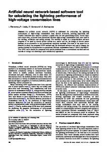
In this section, an explicit design of the approximation based event-triggered controller and NN weight update laws are discussed. A general layout of the event-triggered system is shown in Figure 1. We assume that the sensor transmits the feedback data to the controller via a communication network without any packet loss and delay at the event instants only and the control input is fed directly to the actuator.

gi ,min and gi ,max are known positive constants.

Plant

The i th subsystem Gi of (1) in a simplified form is expressed as zi  k  1  Ai zi  k   Bfi  Z  k  , ui 1  k   + Bgi  Z  k   ui  k  , (3) where

0 1 0 0 A   0 0

0

0 0  m m 1  0

and



,n ,

T

zi , m  k  m , i  1, 2,

nonlinear functions and ui 1  k   u1  k 

satisfies the

(4)

where   (k )    V T x  k  l 1 forms a stochastic basis

the state, input and output vectors. The functions fi ( )  and gi ( )  for all i  1, 2, , n are unknown smooth

i  1, 2,

ud  k   W T  (V T x(k ))   (k ),

Assumption 2: The target weight matrix, the NN activation functions and the reconstruction error are bounded above by a positive constant such that W  Wmax ,  x    max and

znT  k  mn

ui  k   and yi  k   for i  1, 2,

whereas the output layer weights are updated. This class of NN is known as linearly parameterized NN [8]. In terms of NN weights, the control input can be expressed in a compact set   mn as

B  0 0

Sensor/Trigger Mechanism

Network NN based Controller

ZOH

T

1 m .

Weight Update

In this paper, it is assumed that the system dynamics fi  Z  k  , ui 1  k   and gi  Z  k   are completely unknown. Therefore, to implement the control law, NNs are used for their universal approximation property, discussed in the next paragraph. The universal approximation property states that a smooth nonlinear function can be approximated by using a NN in a compact set   mn . In this paper, for approximating each control input, we have considered a two layer NN where the input layer weight matrix is selected at random and held

Figure 1. Event-triggered system with approximation based controller.

Now the following assumption is needed for designing the control law. The unknown nonlinear functions Assumption 3: fi  Z  k  , ui 1  k   , gi  Z  k   and NN activation function

  Z  k  , ui 1  k   are Lipschitz continuous with respect to Z  k  on a compact set   mn . Then for every   mn there exists constants L fi  0 , Lgi  0 , and Li  0 such

2018





that fi  Z  k  , ui (k )   fi Zˆ  k  , ui (k )  L fi Z  k   Zˆ  k  ,



a monotonically increasing sequence of time instant kt t 1 

for all k  such that the events are triggered at the time instants kt or, alternatively, the event-trigger condition is



gi  Z  k    gi Zˆ  k   Lgi Z  k   Zˆ  k  and i  Z  k  , ui (k ) 





i Zˆ  k  , ui (k )  Li Z  k   Zˆ  k  are satisfied.

violated at kt . Clearly, the sequence kt t 1 is a subsequence 

A. Controller and NN Weight Update Law Design Consider the system dynamics (1) wherein the inputs of the system are in a triangular form. Hence, the controller can be designed independently for each subsystem Gi for i  1, 2, n . Consider the subsystem Gi in (3) for i  1, 2, n and an ideal controller of the form -fi  Z  k  , ui 1  k   + Ki zi  k  ud , i  k  = , for i  1, 2, n , (6) gi  Z  k   designed by using feedback linearization technique. The closed-loop dynamics becomes zi  k  1 = Ac,i z  k  , for i  1, 2, n , (7) 1 0 0   0  0 0 0  where Ac ,i  Ai  BKi =  is the closed 1    K i , m   K i ,1 K i ,2 loop system matrix with Ac ,i being Schur by proper Ki , m  for

selection of control gain vector Ki =  Ki ,1 Ki ,2

i  1, 2, n through pole placement design. Implementation of this controller (6) needs the system dynamics fi  Z  k  , ui 1  k   , gi  Z  k   for i  1, 2, n ,

which are considered to be unknown. Instead of approximating the unknown functions individually, we use a single linearly parameterized NN as discussed in the Section II to approximate each control input. Hence, the ideal NNbased control input in a compact set   mn is expressed as (8) ud ,i  k   WiT i i  k     i  k  , for i  1, 2, n , where Wi li 1 is the unknown NN target weight vector, Vi  ali

is the fixed input layer

i   

li 1

weight vector,

is the activation function,  i  k  is the NN

reconstruction error for i  1, 2, n , li is the number of neurons in the hidden layer, a is the number of inputs to the NN

for

i  1, 2,

n,

i  k   Vi  Z T

T

k 

T i 1

u

 k 

T

for

i  1, 2, n is the scaled NN input vector and K i is the control gain vector. In the case of the event-triggered control for a discrete time system, the system state Z  k  is not transmitted

periodically at every sampling time instant k  . The transmission instants or events are determined by the violation of the event-trigger condition (to be designed later) by evaluating the condition at every sampling instant. Define

of k  . Hence, a zero order hold (ZOH) is used to hold the

last transmitted state Z  kt  between two event-triggered instants, i.e., for kt  k  kt 1 . This implies the control input is updated only at the trigger instants and held constant during the inter-event time. This aperiodic transmission of system state can be considered as an error in the system state similar to the measurement error. Defining this error between the current measured state Z  k  and the last transmitted state Z  kt  as the event-trigger state error, e  k   Z  k   Z  kt  , where e  k   e1T  k  e2T  k 

(9) T

enT  k  mn and each

ei  k   zi  k   zi  kt  m for i  1, 2, n . It is important to mention here that the event-trigger state error is discontinuous at the trigger instants kt as the last transmitted state is updated to the current received state, i.e., (10) Zi  kt   Zi  k  for k  kt . Hence, we can rewrite e  k  as  Z  k   Z  kt  , Event is not triggered, kt  k < kt+1 ,  (11) e k    Event is triggered, k = kt .  0,

The ideal control input (8) can be estimated by updating the NN weight vectors. In the event-triggered context, the estimated/ actual control input can be expressed as (12) ui  k   WˆiT  k  i (i  kt ) , where Wˆi  k  li 1 is the NN actual weight vector updated using the aperiodic update law, i   li 1 is the activation T

function and i  kt   ViT  Z T  kt  uiT1  kt  is the scaled NN

input held by the ZOH for i  1, 2, n . The aperiodic weight update law is chosen to be (13) Wˆi  k  1 = Wˆi  k     k  ii i  kt   eiT  k  1 B ,



for all k 



where i  0 is the adaptive learning gain,

i   is the NN activation function i  1, 2,

n , B is a

constant vector as defined earlier, and   k  is an indicator function for the event-trigger instants defined by event is not triggered, kt  k < kt+1 , 0,  k    event is triggered, k = kt . 1,

(14)

The indicator function   k  enables the update law once an

event is triggered at k = kt by becoming one and the NN weights are updated. During the inter-event time kt  k < kt+1 the NN weights are not updated and held at the previous value. Thus, the update law (13) is aperiodic, as

2019

proposed, to reduce computation when compared to traditional NN based methods [8]. B. Closed-Loop System and Error Dynamics Define the NN weight estimation error for the i th control input is Wi  k   Wi  Wˆi  k  . (15) From (15), the dynamics of the weight estimation error are





Wi  k  1 = Wi  k     k  ii i  kt   eiT  k  1 B ,

for all k 

(16)

.

Next, the closed loop dynamics of the i th subsystem Gi in (3) along with the controller (12) for the case with event is not triggered, i.e., kt  k  kt 1 is given by zi  k  1  Ai zi  k   Bfi  Z  k  , ui 1  k   + Bgi  Z  k  

WˆiT  k  i i  kt   .

Adding

Wˆi

and

subtracting

ud ,i  k 

from

(6)

 k i (i  k ) , the closed-loop dynamics become zi  k  1  Ac,i zi  k   Bgi  Z  k  WiT i (i  k )  Bgi  Z  k  

and

T





 WˆiT  k  i (i  k )  i (i  kt )    i  k  ,

(17)

where Ac,i  Ai  BKi . Since, from (11) the event-trigger error at the trigger instants becomes zero, i.e., e  k   0 the closed-loop dynamics for the case an event is triggered , k  kt from (17) turns out to be zi  k  1  Ac ,i zi  k   Bgi  Z  k  WiT i (i  k ) (18)  Bgi  Z  k    i  k  , for k  kt . Finally, the event-trigger state error dynamics for the i th subsystem is given by (19) ei  k  1 = zi  k  1  zi (kt ).

IV. MAIN RESULTS This section discusses the design of the event-trigger condition which ensures the approximation of the control input and ultimate uniform boundedness (UUB) of the closed-loop system parameters. A. Event-Trigger Condition Design The design of the event-trigger condition is crucial and involved because of the approximation based event-triggered control. In contrast with the traditional event-triggered control design [2]-[6], the approximation based design necessitates the consideration of additional errors, such as rate of change of the event-trigger state error, eiw1  k   ei  k   ei  k  1 and error in the control input due to NN weight estimation in an event-trigger context eiw2  k   WˆiT  k     k  1     kt   for i  1, 2, n ,

  ET : D  max  e 1i  n

3

the

identity

matrix

ei  k  1  ei  k   Ac ,i zi  k   Bgi  Z  k  WiT  k  i (i  k )



Similarly,

(20)

event-trigger error dynamics are rewritten from (20) as ei  k  1  Ac ,i zi  k   Bgi  Z  k  WiT  k  i (i  k )

 Bgi  Z  k    i  k  .

1i  n

1i  n

varying

i

i

(24)

i

i

(25)

thresholds



coefficients,

for

i  1, 2,

i  k   with

n

1/ 2

    i min  Qi  gi ,mini ,min c1s1 i  k     2   2 2 2  2 ˆ  gi ,max Pi  24i,max (1  gi,max )  6 Li gi,mini,min Wi  k      

  i min  Qi  C1S 2 i  k     gi2,max 12 i2i4,max Pi  6 L2 Pi Wˆi  k  i 



,

1

2



2    

n . The positive definite symmetric matrices Pi

for i  1, 2,

 k  i (i  k )  i (i  kt )    i  k   . when an event is triggered, i.e., e  k   0 the

 Bgi  Z  k   Wˆi

T

time

(23)

  min    k  z  k   ,  k     min    k  z  k   .



and

zi  kt   zi  k   e  k  . Then we have



min ic1s1  k  , ic1s 2  k 



is

w2 i

1i  n

The

 WˆiT  k  i (i  k )  i (i  kt )    i  k   zi  kt  ,

Im

1i  n

ET2 : D max eiw1  k 

ei  k  1  Ac ,i zi  k   Bgi  Z  k  WiT i (i  k )  Bgi  Z  k  

with Ac,i = Ac,i - I m ,



ET1 : D  e  k    min i  k  zi  k  ,

Along the system dynamics (3), when an event is not triggered, i.e., for kt  k  kt 1 , (19) is expressed as







to ensure the approximation of the control input and stability of the closed-loop event-triggered system. In other words the event-trigger condition should ensure suitable number of events to approximate the control input faster and at the same time maintaining the stability and desired performance. With this effect, define the event-trigger condition as (22) ET1  ET2  ET3 , and the events are triggered at the violation of the condition (22), where  is the logical OR operator and ET1, ET2 and ET3 are given in the following equations

and Qi satisfies the Lyapunov equation AcT,i Pi Ac,i  Pi  Qi with

Ac ,i  2 Ac ,i

0  i  2

2 i ,min



and

the

gi ,min 1  gi ,max  3

zone operator D   is defined as (21)

Next, the main results of the event-triggered control design are introduced. 2020

learning

 ; if Z  k   Bz D    0; otherwise

3 i ,max

g

2 i ,max

gain

. The

satisfies dead-

(26)

where Bz is the desired ultimate bound of the system states which can be achieved by increasing the number of neurons in the hidden layer of the NN. Remark 1: The Lyapunov equation

AcT,i Pi Ac,i  Pi  Qi

guarantees a positive definite solution Pi for a given a

positive definite Qi as the matrix Ac,i  2  Ai  BKi  is Schur and can be achieved by selecting suitable the control gain K i . Remark 2: The event-trigger condition in (22) is a function of (a) the event-trigger state error, (b) change in the eventtrigger state error if there is no triggering at consecutive time instants, and (c) the error in the control inputs due to event based transmission and estimation. The condition in (22) is designed from the Lyapunov based stability proof. If any of





these errors exceeds the threshold, i.e., min i  k  zi  k  , 1i  n

the system states are transmitted and the control inputs are updated in order to maintain system stability. In addition, these conditions ensure the approximation of the control inputs by generating required number of events at the initial learning phase while ensuring the system stability. Remark 3: The NN weights are updated simultaneously both at the sensor and the controller since the event-trigger condition uses the estimated NN weights i.e., i( ) is a function of Wˆ . Note all the data are available at the sensor i

to update the NN weights at the sensor. Remark 4: The dead-zone operator resets the event-trigger error to zero to stop unnecessary triggers as long as the system state remains in the ultimate bound. Next the following lemma is useful for proving the theorem. Lemma 1: Consider the MIMO nonlinear discrete time system (1) along with the approximation based controllers (12) for i  1, 2, n . Let the sensor transmits the state vector at the violation of the event-trigger condition (22) and let the weights be updated using (13) for i  1, 2, n . Then, the following inequality holds 2 1 WiT  k   ei  k   ei  k  1  Ac,i zi  k  1  B gi ,mini ,min (27)



2  gi  Z  k  1  WˆiT  k  i (i  k  1) i (i  kt )   i  k  1  ,

when there are no events occurring between two consecutive time instants. Next, the main result of the event-triggered design is introduced in the theorem. B. Boundedness of the Closed-loop System Theorem 1: Consider the MIMO nonlinear discrete time system (1) along with the approximation based control input (12). Let the NN weights Wˆi  0  li 1 be initialized in the

compact set   mn and the Assumptions 1-3 hold. Then there exist constants i  0 such that the closed-loop eventtriggered MIMO nonlinear discrete time system state vector mn Z k for any initial condition in the compact set    and the NN weight estimation errors Wi  k  are uniformly ultimately bounded (UUB) provided the events are triggered by the violation of event-trigger condition (22) while the NN weights are updated using (13). Remark 5: The stability of the closed loop event-triggered system is demonstrated by proving the stability in the following two cases: (a) event is not triggered and (b) event is triggered at time k for all k  by using Lyapunov direct method. Further, to analyze the growth of control input approximation error and allow the NN to approximate the control inputs faster, we consider the effect of previous time instant, k  1 , when an event is not triggered at present time k . In the next section simulation results are presented to validate the analytical design. V. SIMULATIONS In this section, we have considered a numerical example of the form as in (1) to validate the analytical design of the event-triggered control. Consider the nonlinear system  x1,1  k  1  x1,2  k   G1   x1,1 (k )  x1,2  k  1  1  x3 k  x 2 k  x 2 k  u1 (k ) 1,2   2,1   2,2   

 x2,1  k  1  x2,2  k   G2  u1 (k ) x2,1 (k ) (28)  x2,2  k  1  1  x 2 k  x 2 k  x 2 k  u2 (k ) 1,1   1,2   2,2    with a sampling time of 0.01 sec. The controllers u1  k   and u2  k   for both the subsystems G1 and G2 are implemented by using two-layer linearly parameterized NNs as in (12) with 45 and 25 neurons respectively. The input weight vectors V1 445 and V2 525 are selected at random from a uniform distribution in the interval 0 to 1 and the output layer weight vectors W1 45 and W2 25 are chosen at random in the interval 0 to 0.06. Sigmoid activation functions are used, i.e., tanh( ) for both the NNs. The Lipschitz constants for the activation function computed to be 6.88 and 4.75. Learning gains are selected as 0.017 and 0.095 respectively. The ultimate bound on the system states is chosen to be 0.001. The parameters   .99 , Q1  100* I 2 , Q2  20* I 2 and

gi ,min  gi ,max  1 , with i  1, 2 . Initial system states are taken to be

 0.05

0.5 0.5 0.2 , the control gains T

K1  0.2 0.3 and K2  0.5 0.1 . The event conditions are obtained by using (22). The system is simulated for 5 sec., i.e., 500 sampling instants.

2021

System States(Z)

1

z11

0.5

z12

z21

system states stay in the bound can be clearly seen from Figure 3 (bottom). Hence, the plot flattens after 300 sampling instants, further, indicating fewer events. NN Weight Estimation(||W||)

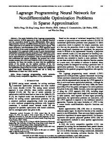
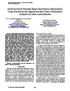
The system response is shown in Figure 2. The states are converging to near zero implying the stability and desired performance is achieved. The event-based approximated control inputs, Figure 2 (bottom), show the aperiodic update of the inputs as a step and finally converge to near zero along with the convergence of the system state. z22

0

Control Inputs(u)

-0.5 0 0.5

1

2

3

4

5 u1

1

2 3 Time (Sec)

4

5

Threshold

Cumulative Num. of Triggering

0 0

100

200

300

400

400

500

Inter-event Time

200 0 0

100

200 300 Sampling Instants(k)

400

0.15

NN Weight(||W2||)

0.1 0.05 0 0

1

2 3 Time (Sec)

4

5

VI. CONCLUSIONS In this paper, we proposed an approximation based controller design in the event-triggered context for a MIMO uncertain nonlinear discrete-time system. This approach reduced the complexity and computational load by using a single NN for each control input when compared to system identification with multiple NNs. In turn, the knowledge of the system dynamics is not required. Design of the eventtrigger condition by taking the constraints due to NN approximation and the event-triggered transmission into account is also presented. The analytical results are augmented with the simulation results prove the validity.

Threshold Trigger Instants

0.01

NN Weight(||W1||)

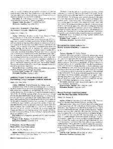
As proven in the Theorem 1, the convergence of the NN weight vectors to a constant value, or alternatively, the boundedness of the NN weight estimation error is shown in Figure 4.

Figure 2. (Top) Convergence of system states, (bottom) approximated control input of the nonlinear event-triggered control system. 0.02

0.2

Figure 4. Boundedness of the NN weights.

u2 0 0

0.25

500

Figure 3. (Top) Performance of the nonlinear event-triggered controller showing threshold and triggering instants, (bottom) cumulative number triggers instants indicating reduction in transmission.

The performance metric in terms of evolution of eventtrigger threshold and the number of events are shown in Figure 3. Figure 3 (top) shows the reduction in the trigger instants as the system evolves and the NNs learn the ideal control input. The crowded red vertical lines initially indicate triggered events at almost every sampling instant because of the large NN weight estimation error. Once the control inputs are approximated by the NN-based controllers, i.e., the NN weight vectors converged to the bound, the triggered events are reduced. This is shown by the gaps in the triggers instants in Figure 3 (top). Figure 3 (bottom) depicts the cumulative number of trigger instants and the inter-event duration. The horizontal step size shows the inter-event duration and the y-axis shows cumulative number of triggered events within the simulation time. A total number of triggered events observed are 231 out of 500 sampling instants. In other words, the computation required in terms of updating the control input and the NN weights is less in comparison to the traditional NN based control. Further, this also reduces the network traffic which is directly proportional to the number of triggered instants. The effect of the dead-zone-operator which resets the event-trigger error to zero as long as the

REFERENCES [1]

K. Astrom and B. Bernhardsson, “Comparison of Riemann and Lebesgue sampling for first order stochastic systems,” in Proc. IEEE Conf. Decision Control, vol. 2, 2002, pp. 2011–2016. [2] P. Tabuada, “Event-triggered real-time scheduling of stabilizing control tasks,” IEEE Trans. on Autom. Control, vol. 52, pp. 16801685, 2007. [3] A. Eqtami, D. V. Dimarogonas, and K. J. Kyriakopoulos, “Eventtriggered control for discrete-time systems,” in Proc. Amer. Control Conf., 2010, pp. 4719-4724. [4] C. Stocker and J. Lunze, “Event-based control of nonlinear systems: An input-output linearization approach,” in Proc. joint IEEE Conf. Decision Control and Eur. Control Conf., 2011, pp. 2541–2546. [5] M. Mazo, and P. Tabuda, “Decentralized event-triggered control over wireless sensor/actuator networks,” IEEE Trans. on Autom. Control, vol. 56, pp. 2456-2461, 2011. [6] D. V. Dimarogonas and K. H. Johansson, “Event-triggered control for multi-agent systems,” in Proc. joint IEEE Conf. Decision Control and Chinese Control Conf., 2009, pp. 7131–7136. [7] A. Sahoo, Hao Xu, and S. Jagannathan, “Neural network-based adaptive event-triggered control of affine nonlinear discrete time systems with unknown internal dynamics,” in Proc. Amer. Control Conf., 2013, pp. 6433-6438. [8] S. Jagannathan, Neural network of nonlinear discrete-time systems. CRC Press, 2006. [9] Hao Xu, S. Jagannathan and F. L. Lewis, “Stochastic optimal control of unknown linear networked control system in the presence of random delays and packet losses,” Automatica, vol. 48, pp. 10171030, 2012. [10] J. Zhang, S.S. Ge, and T.H. Lee, “Output feedback control of a class of discrete MIMO nonlinear systems with triangular form inputs,” IEEE Trans. on Neural Netw., vol. 16, pp. 1491-1503, 2005.

2022