Neural Network based Segmentation of Magnetic ... - CiteSeerX

Neural Network based Segmentation of Magnetic Resonance Images of the Brain Javad Alirezaie1 , M. E. Jernigan2 , and C. Nahmias3 1 2Department of Systems Design Engineering, University of Waterloo, Waterloo, Ontario, Canada N2L 3G1. 3 Department of Nuclear Medicine, McMaster University, Hamilton, Ontario, Canada L8N 3Z5. ;

Abstract This paper presents a study investigating the potential of arti cial neural networks (ANN's) for the classi cation and segmentation of magnetic resonance (MR) images of the human brain. In this study, we present the application of a Learning Vector Quantization (LVQ) Arti cial Neural Network (ANN) for the multispectral supervised classi cation of MR images. We have modi ed the LVQ for better and more accurate classi cation. We have compared the results using LVQ ANN versus back-propagation ANN. This comparison shows that, unlike back-propagation ANN, our method is insensitive to the gray-level variation of MR images between dierent slices. It shows that tissue segmentation using LVQ ANN also performs better and faster than that using back-propagation ANN.

I. Introduction Segmentation of images obtained from magnetic resonance (MR) imaging techniques is an important step in the analysis of MR images of the human body. MR imaging has a unique advantage over other modalities in that it can provide multispectral images of tissues with a variety of contrasts based on the three magnetic resonance parameters , T1, and T2 [1]. Tissue classi cation of normal and pathological tissue types using multispectral MR images has great potential in clinical practice. Possible areas of application include the automatic or semiautomatic delineation of areas to be treated prior to radiosurgery, and the delineation of tumors before and after surgical or radiosurgical intervention for response assessment. Tissue classi cation is also of importance in the study of neuro degenerative diseases such as Alzheimer's disease and multi-infarct dementia [2]. In these studies, the quantities of interest are the volumes of white matter, gray matter, cerebrospinal uid, and abnormal tissues. \Because the manual delineation of white and gray matter on a large number of MR images is impractical, detection of their structure boundaries and computation of

their volume only becomes possible when reliable and robust methods are developed to assist human experts." [3] Multispectral analysis has been the most successful approach to the automatic recognition of tissue types in the human body based on MR imaging [4]. During the last few years, several studies on the automatic recognition of normal tissues in the brain and its surrounding structures have been published [5], [6], [7], [8], [9], [10], [11], [12], [13],[14], [15], [16]. However, none of these methods give consistently adequate results [3]. One of the major problems in the classi cation is intensity variations that are introduced by inhomogeneities in the radio frequency eld and these can occur within or between slices in the same patient as well as between patient studies. This problem has hampered the development of fully unsupervised techniques. In addition, there is no accepted method to validate and measure the accuracy of ant algorithm. Nevertheless, classi cation techniques that do rely on operator interventions, and which therefore are subjective, have found applications in speci c cases [3]. It has been the purpose of this study to explore the potential of Learning Vector Quantization (LVQ) Arti cial Neural Networks (ANN) in the classi cation and segmentation of magnetic resonance (MR) images of the brain. This approach has attracted considerable attention in the recent past [17] and was proposed by Kohenen [18]. This type of network is proposed here for the classi cation and segmentation of tissues in MR brain images. This study is an extension of the authors' earlier work [19]. The main dierences are 1) the utilization of spatial information 2) an extensive comparison of the back-propagation ANN and learning vector quantization ANN and 3) the use of LVQ ANN for an adaptive learning scheme capable of overcoming inter-slice and interpatient intensity variations. We use multispectral MR images and demonstrate an improved dierentiation between normal tissue types of the brain and surrounding structures using pixel intensity values and spatial information of neighboring pixels. We give the essential steps of the training technique, and show how the LVQ ANN can be used for classi cation and segmentation of dierent tissues. We present results obtained from our method and compare it with back-propagation arti cial neural networks. The paper

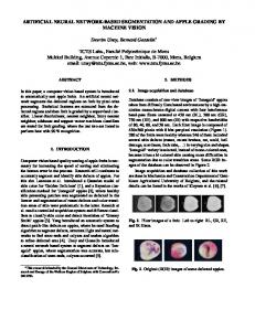
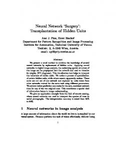
si es patterns by using an optimal set of reference vectors or codewords. A codeword is a set of connection weights from input to output nodes (Figure 2). The set of vectors w1; w2; :::; wk is called a codebook in which each vector wi is a codeword for Vector Quantization. If several codewords are assigned to each class, and each is labeled with the corresponding class symbol, the class region in the x space (input) is de ned by simple nearest-neighbor comparison of x with the codewords wi ; the label of the closest wi de nes the classi cation of x. (a) (b) To de ne the optimal placement of wi in an iterative learning process, initial values must be set. The next phase, then, is to determine the labels of the codewords, by presenting a number of input vectors with known classi cation, and assigning the codewords to dierent classes by majority voting, according to the frequency with which each wi is closest to the calibration vectors of a particular class. The classi cation accuracy improves if the wi are updated according to the algorithm described below. [20], [21]. The idea is to pull codewords away from the deci(c) sion surface to mark (demarcate) the class borders more Figure 1: (a): A T1-weighted image (b) A T2-weighted accurately. In the following algorithm we assume wi is the nearest codeword to the input vector x (Eq. 1) in the Euimage (c) A -weighted image. clidean metric; this, then, also de nes the classi cation of x. concludes with some discussion and comments. jjx ? wi jj = MINjk=1 jjx ? wj jj (1) where the Euclidean distance between any two vectors X and Y is de ned as II. MR Brain Images n X Standard 256256 pixel transverse T1, T2, and -weighted (xi ? yi )2 ] 12 jj X ? Y jj = [ spin echo images acquired with a 1.5 Tesla GE MR scanner i=1 have been used in this study. Images were selected from a large series of axial images of the whole head. The image The following algorithm shows how the codewords will slices were 5 mm thick with 2.5 mm inter-slice space. The be updated. eld of view was 22 cm, resulting in a pixel size of about 0:8  0:8 mm2. wi (t + 1) = wi(t) + (t)[x ? wi (t)] (2) Because the T1 weighted images were acquired with a eld of view equal to 20 cm, they were resampled to ensure if x is classi ed correctly (if the label agreed with accurate registration. A bilinear polynomial method was codeword assignment), used for the interpolation. The set of multispectral images wi (t + 1) = wi(t) ? (t)[x ? wi (t)] (3) were acquired using the following parameter combinations. TR/TE = 2916 ms/ 17 ms for the -weighted, TR/TE = 2916 ms/ 119 ms for the T2 and TR/TE = 600 ms / 16 if the classi cation of x is incorrect (if the label does not agree with the codeword assignment), and ms for the T1 weighted images respectively. A typical slice from the brain of a normal volunteer is wj (t + 1) = wj (t) ; i 6= j (4) shown in Figure 1(a), 1(b), 1(c). (the other codewords are not modi ed). III. Methods Here (t) is a learning rate such that 0 < (t) < 1, and is decreasing monotonically in time. We chose A. LVQ Classi er t ) Learning Vector Quantization ANN is a classi cation net(t) = 0:2(1 ? 10000 work that consists of two layers. The two layer ANN clasy The original image slices are 256  256 pixels and are reduced by After enough iterations, the codebook typically confactor 2.25 in Fig. 1. verges and the training is terminated. y

Features from T1-weighted Image Features from T2-weighted Image

Class 1

{ { {

Class 2

Features from PD-weighted Image

w

. . . . .

i

Input Layer

.. .. Class 7

Figure 2: Topology of LVQ ANN

B. Back-propagation ANN classi er

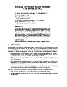
The back-propagation ANN which is used in this study consists of one input layer, two hidden layers, and one output layer. Figure 3 shows the topology of the network. The number of input and output nodes are equal to 9 and 7 respectively. The number of nodes in each hidden layer is 18. Figure 3 shows the topology of the network. The training of the network consists of nding a map between a set of input values and a set of output values. This mapping is performe by adjusting the value of the weights wij using a learning algorithm. The popular learning algorithm, the generalized delta rule brie y introduced here (see [22]) is used. After the weights are adjusted on the training set, their value is xed and the ANN is used to classify input vectors. Assume the input vector, xi = (xi1; xi2; :::; xiN ) is applied to the input units and the output vector, oi is the observed output vector. The generalized delta rule minimizes an error term E which is de ned as N X (5) Ei = 21 (xij ? oij )2 j

The error term is a function of the dierence between the output and input vectors. This dierence can be minimized by adjusting the weights wij in the network. The generalized delta rule implements a gradient descent in E to minimize the error [22]. wjk then presents as follow,
iwjk = ij oik (6) with  P ij ) p ip wpj for a hidden node (7) ij = f(x(net ij ? oij )f (netij ) for an output node P in which netij = p wjkoik + j is the total input to node j including a bias term j and the parameter is the learning rate. The output of node j due to input k is thus oij = fj (netij ) with f the activation function. If 1 ?z , equation (7) can be rewritten as, f(x) = 1+exp  o (1 ? o ) P  w for a hidden node ij = (xij ? o ij)o (1p ?ipo pj) for an output node ij ij ij ij (8) 0

{ { {

Class 2

Features from T2-weighted Image Features from PD-weighted Image

w

.. . ..

.. .. .

.. .. .

i

Input Layer

Kohonen Layer

0

Class 1

Features from T1-weighted Image

Class 7 Hidden Layer

Hidden Layer

Output Layer

Figure 3: Topology of the back-propagation ANN Finally, by adding a momentum term to the learning rate we obtain for the weights
i wjk[n] = ij oik + i wjk[n ? 1]

(9)

where  is the momentum rate at each iteration, the weights are thus modi ed as follows: wjk[n + 1] = wjk [n] +
i wjk[n]

(10)

IV. Experiment and Results In this section we present the results from two approaches for classi cation of tissue types in MR images of the head. In both methods we use pixel intensity values and spatial information of neighboring pixels as features. The number of input nodes in the network is equal to the number of features and the number of output nodes is equal to the number of target tissue classes. In each of the cases presented in this work, the images were classi ed into seven classes: background, cerebrospinal uid (CSF), white matter, gray matter, bone, scalp and lesion or tumor (if present).

A. Results of LVQ ANN Approach

Codebook Initialization: For the initialization of the code-

book vectors a set of vectors is chosen from the training data, one at a time. All the entries used for initialization must fall within the borders of the corresponding classes, and this is checked by the K-nearest neighbor (K-nn) algorithm. In fact in this step the placement of all codebook vectors is determined rst without taking their classi cation into account. The initialization program then selects the codebook vector based on the desired number of codewords. For our segmentation problem, dierent sets of codebooks including 60 to 120 codewords for each set have been tested. The accuracy of classi cation may depend on the number of codebook entries allocated to each class. There does not exist any simple rule to nd out the best distribution of the codebook vectors. We used the method of iteratively balancing the medians of the shortest distances in all classes. Our program rst computes the medians of the

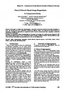
shortest distances for each class and corrects the distribution of codewords so that for those classes in which the distance is greater than the average, codewords are added; and for those classes in which the distance is smaller than the average, some codewords are deleted from the initialized codebook vector. When the codebook has been initialized properly, training is started. Training vectors are selected by manual segmentation of a Multi-spectral MR images (T1, T2, and -weighted images) of the head. In a typical experiment, the T1-weighted images are displayed on the computer screen, one slice at a time. Next, representative regions of interest (ROI's) for the target tissue classes are selected interactively on the computer screen using a mouse-driven interface. When the ROI's are selected, a data structure containing the labels of the regions, the spatial information of neighboring pixels in these regions, and the corresponding intensity vectors is created and stored in a le. The created le is then used to train the neural networks. Figure 4 shows results obtained using this approach. The original proton density image is shown in Figure 4(a). A complete segmented image is shown in Figure 4(b); CSF, white matter and gray matter are shown separated in Figure 4(c), 4(d) and 4(e).

(a)

(b)

(c)

(d)

(e)

B. Results of Back-propagation ANN Approach

The rst step to use the network was to determine the learning parameters. Fig. 3 illustrates the topology of the network. With that topology, the network was trained three times with dierent learning rates and momentum. The eect of the learning parameter and momentum rate on the speed of convergence was investigated, and the best combination was selected for classi cation and segmentation. The same training and test data were used for training and testing the network. The training was stopped if convergence was not reached after 100,000 iterations. In order to investigate the impact of the topological parameters on both the speed of convergence, and the classi cation accuracy several experiments have been set up. Neural networks with one and two hidden layers were generated, and the number of nodes in each of the layers was varied from 10 to 30. From results obtained in each test the best combination is selected for classi cation and segmentation of MR images. Results were acquired from this technique are shown in Fig. 5. Fig. 6 shows the results of segmenting an MR image of a patient study with tumor. The patient had a malignant glioma. In this case the segmentation of the MR images is complicated because image features of abnormal tissues may be very close to those of their neighbor normal tissues. Therefore, abnormal tissues may be found in a normal tissue component after a segmentation. Abnormal tissues may also deform the geometry of normal tissues. It can be observed that the results for back-propagation ANN suer from noise and mis-classi cation and that the

Figure 4: (a) The original -weighted image, (b) A complete segmented image using LVQ ANN (c) CSF tissues (d) white matter (e) gray matter LVQ ANN results are quite good.

V.

Discussion and Conclusion

It has been found that back-propagation neural networks are very sensitive to the training set in MR image segmentation of the brain. Back-propagation nets provide adequate brain segmentations provided that the training data are quite good. They can learn eectively on as few as 250 pixels per class in a 256x256 MR image using a multi-layer back-propagation network with between ten and 20 hidden units, which means that training and testing are relatively fast. Eort to nd a universal training set that would be useful on many dierent MR images has been made. However, because of the intensity variation across MR images which causes instability on training data , the backpropagation network could not perform well every time. If back-propagation networks are to be used for segmentation of MR images, at least for now, reliance on operator

(a)

(a)

(b)

Figure 6: (a) Segmentation of Tumor in an abnormal brain using back-propagation ANN (b) Segmentation of Tumor using LVQ ANN

References (b)

(c)

[1] R. R. Edelman and S. Warach. Magnetic resonance imaging ( rst of two parts). the New England Journal of Medicine, 328:708{716, March 1993. [2] W. Bondare, J. Raval, B. Woo, D. L. Hauser, and P. M. Colletti. Magnetic resonance imaging and the severity of dementia in older adults. Arch. Gen. Psychiatry, 47:47{51, Jan. 1990.

(d)

(e)

Figure 5: (a) The original -weighted image, (b) A complete segmented image using back-propagation ANN (c) CSF tissues (d) white matter (e) gray matter intervention to select good training data for each subject and each slice of data is crucial. In this paper we have demonstrated that the three normal tissue types of the brain can be recognized automatically by multispectral analysis of MR images. Furthermore, our results are not limited to MR images recorded from a single patient, and the classi cation procedure is valuable for MR images recorded from other patients. Our method is insensitive to the variations of gray-level for each tissue type between dierent slices from the same study. In conclusion, the present study indicates that ANN are a particularly good choice for segmentation of MR images because their generalization properties require the labeling of only few training points, and they produce results faster than other traditional classi ers. We showed that tissue segmentation using LVQ ANN produces better and faster than back-propagation ANN and is a powerful technique for MR image segmentation.

[3] B. M. Dawant, Alex P. Zijdenbos, and Richard A. Margolin. Correction of intensity variations in MR images for computer-aided tissue classi cation. IEEE Transactions on Medical Imaging, 12(4):770{781, December 1993. [4] T. Taxt and A. Lundervold. Multispectral analysis of the brain using magnetic resonance imaging. IEEE Engineering in Medicine and Biology, 13(3):470{481, Sept. 1994. [5] S.C. Amartur, D. Piraino, and Y. Takefuji. Optimization neural networks for the segmentation of magnetic resonance images. IEEE Transactions on Medical Imaging, 11(2):215{220, June 1992. [6] H. S. Choi and Y. Kim. Partial volume tissue classi cation of multichannel magnetic resonance images- a mixel mode. IEEE Transactions on Medical Imaging, 10(3):395{407, September 1991. [7] C. Li, D. B. Goldgof, and L. O. Hall. Knowledge-based classi cation and tissue labeling of MR images of human brain. IEEE Transactions on Medical Imaging, 12(4):740{750, September 1991. [8] M. C. Clark, L. O. Hall, D. B. Goldgof, L. P. Clarke, R. P. Velthuizen, and M. S. Silbiger. MRI segmentation using fuzzy clustering techniques. IEEE Engineering in Medicine and Biology, pages 730{742, Dec. 1994.

[9] M. W. Vannier, M. Gado, and R. L. Butter eld. Mul- [22] J. A. Freeman and D. M. Skapura. Neural Nettispectral analysis of magnetic resonance images. Raworks, Algorithms, Applications, and Programming diology, 154(1):221{224, 1985. Techniques. Addison-Wesley Publishing Company, 1991. [10] R. M. Haralick and L. G. Shapiro. Survey image segmentation techniques. Computer Vision, Graphics, and Image Processing, 29:100{132, 1985. [11] D. A. Ortendhal and J. W. Carlson. Segmentation of magnetic resonance images using fuzzy clustering. In C.N. de Gra and M. A. Viergever, editors, Information Processing in Medical Imaging, pages 91{106. Plenum Press, New York, 1988. [12] L. P. Clarke, R. P. Velthuizen, S. Phuphanich, J. D. Schellenberg, J. A. Arrington, and M. Silbiger. MRI: Stability of three supervised segmentation techniques. Magnetic Resonance Imaging, 11:95{106, 1993. [13] L. O. Hall, A. M. Bensaid, R. P. Velthuizen L. P. Clarke, M. S. Silbiger, and J. C. Bezdek. A comparison of neural network and fuzzy clustering techniques in segmenting magnetic resonance images of the brain. IEEE Transactions on Neural Networks, 3(2):672{682, September 1992. [14] E.J. Dudewicz, G. C. Levy, M. J. Rao, and F. W. Wehrli. Advanced statistical methods for tissue characteristics. Magnetic Resonance Imaging, 2:1988, 1988. [15] M. I. Kohn, R. C. Gur, and G. T. Herman. Analysis of brain and cerebrospinal uid volumes with MR imaging. Radiology, 178(1):115{122, 1991. [16] T. Taxt, A. Lundervold, B. Fuglaas, H. Lien, and V. Abeler. Multispectral analysis of uterine corpus tumors in magnetic resonance imaging. Magnetic Resonance in Medicine, 23:55{76, 1992. [17] N. R. Pal, J. C. Bezdak, and E. C. K. Tsao. Generalized clustring networks and kohonen's self-organizing scheme. IEEE Transactions on Neural Networks, 4(4):549{557, July 1993. [18] T. Kohonen. An introduction to neural computing. Neural Networks, 1:3{16, 1988. [19] J. Alirezaie, C. Nahmias, and M. E. Jernigan. Multispectral magnetic resonance image segmentation using lvq neural networks. In Proceeding of Int. Conf. on System, Man and Cybernetic, volume 2, pages 1665{ 1670, Oct. 1995. [20] T. Kohonen, G. Barna, and R. Chrisley. Statistical pattern recognition with neural networks: Benchmarking studies. In IEEE International Conference on Neural Networks (ICNN), volume 1, pages 61{68, July 1988. [21] T. Kohonen. Self-Organization and Associative Memory. Springer-Verlarg, 1989.