Neural Network Based Trajectory Planning for Tip Tracking of a Two-Link Flexible Robot Manipulator Gülay Öke and Yorgo İstefanopulos Department of Electrical-Electronic Engineering, Boğaziçi University Bebek, İstanbul, 34342, Turkey e-mail:
[email protected],
[email protected]
Abstract-The main problem in the control of flexible manipulators is to provide precise tip tracking in the operational space. Even if joint angles are controlled sucessfully, the end effector of the manipulator deviates from the desired position because of link deflections and vibrations. In this study, a neural network based trajectory planning method is applied to calculate modifications in the command values of joint angles for tracking control problem, so that the position error of the tip of the manipulator in the operational space is minimized. A PD controller is applied for the joint angle control, where the reference inputs are the modified values calculated by the neural network. Simulations are performed to evaluate the performance of the trajectory planning method and the control procedure. Index terms-flexible manipulator, neural network, trajectory planning.
I. INTRODUCTION Research on flexible manipulators is being carried out for the last two decades, because of the application potential they offer due to the advantages they have over rigid robots. Flexible manipulators have a higher ratio of the load to arm weight. They require less power to produce the same acceleration as rigid link manipulators which have the same load carrying capacity, therefore smaller and cheaper actuators are sufficient. On the other hand, modelling and control of flexible link manipulators are more difficult than for rigid links. The resulting model is a distributed parameter system of infinite dimensions and it is non-minimum phase. The number of control inputs is less than the number of variables to be controlled since the actuators are colocated at the joints. This means that the link deflections can be suppressed only indirectly. The gross motion and the deformational behaviour of the link interact, causing the dynamical equations to be complicated and highly nonlinear. As the spatial boundary conditions of the links change, the characteristic frequencies and modes are modified.
In the technical literature, most of the work on control of flexible manipulators aims at suppression of link deflections, while controlling joint angles simultaneously. Link deflections cannot be controlled directly because of the colocated nature of the actuators, leading to imperfect vibration suppression. Another possible approach is to calcuate new joint angles, to make the tip of the manipulator track the desired trajectory in the operational space, irrespective of link deflections. In this study, a neural network is used to calculate an incremental modification on the command values of joint angles, so that the error of the tip position in the operational space is minimized. A neural network is utilized is to make use of the learning properties of intelligent structures. With the modified trajectory as the new command trajectory in the joint space, a PD controller is applied for joint angle control. Simulations are performed to illustrate the performance of the method on the joint motion, deflections, tip motion and errors in operational space. II. ROBOT DYNAMICS AND KINEMATICS The manipulator which is to be controlled in this study is a planar, two-link flexible manipulator. The model has been derived by De Luca and Siciliano [1] and a sketch of it is given in figure 1. Rotary joints are subject only to bending deformation in the plane of motion; torsional and gravitational effects are neglected.
FIGURE 1. Two-link, planar flexible manipulator
For the two-link flexible manipulator clamped at the origin, depicted in figure 1, the following coordinate ∧ ∧ frames are established: The inertial frame, X 0 , Y 0 ; the rigid body moving frame associated to link i , ( X i , Yi ) and the flexible body moving frame associated to link i , ∧ ∧ . The rigid motion is described by the joint angles X ,Y i i θ i and yi ( xi ) denotes the transversal deflection of link i
at abscissa xi . ( 0 ≤ x i ≤ li ; where l i is the length of link i ).
The closed-form dynamic equations of the robot can be obtained by calculating the kinetic and potential energies and applying Lagrange equations:
.. . B(q ) q + h q, q + Kq = Qu
(1)
where B( q) is the positive definite symmetric inertia . matrix, h q, q is the vector of Coriolis and centrifugal forces, K is the stiffness matrix, Q is the input weighting matrix, u is the n-vector of joint (actuator) torques.
(
q = θ 1 ......θ n δ 11 .......δ 1,m1 ..........δ n ,1 ..........δ n ,mn
)
T
describes the N-vector of generalized coordinates N = n + ∑ mi . Input weighting matrix Q , is in the
(
form
[I
)
i
n×n
0 n×( N−n )
]
T
due
to
the
clamped
link
assumption. This form of the Q matrix implies that inputs can be applied through actuators and they affect only the joint angles directly but not the deformation of the links. To describe the tip position of the robot in operational space, the kinematic equations of the robot are utilized. There are two kinds of rotation matrices for the flexible robot manipulator: The joint (rigid) rotation matrix R i , and the rotation matrix of the flexible link at the endpoint Ei .
cosθ i Ri = sin θ i
1 Ei = yie′
− sin θ i cosθ i
− yie′ 1
(3)
∂ y yie′ = i ∂ xi x = l
In these formulas,
i
(2)
and the linear
i
approximation arctan( yie′ ) ≅ yie′ is valid for small deflections. Ti denotes the global transformation matrix
∧
∧
from X 0 , Y 0 to
( X i , Yi ) , where i represents the i
th
link, and obeys the following recursive equation: ∧
Ti = Ti −1 E i −1 R i = T i −1 R i
∧
T0 = I
(4)
By using (2)-(4), the kinematics of any point along the arm can be fully characterized with respect to the base frame. For the two-link, planar, flexible arm, the position of the tip of the robot in the operational space is given by:
l l p = T1 1 + T1E1T2 2 y1 (l1 ) y2 (l2 )
(5)
where l 1 and l 2 are the lengths of shoulder and elbow links respectively. The p vector denotes the x and y coordinates of the tip of the manipulator:
x p = y
(6)
Using (5), the x and y coordinates of the tip of the manipulator are calculated as follows: x = l1 cosθ 1 − y1 sin θ 1 + l2 cos( θ 1 − θ 2 ) − l2 y1′e sin( θ 1 − θ 2 ) − y2 sin( θ 1 − θ 2 ) − y2 y1′e cos( θ 1 − θ 2 )
(7)
y = l1 sin θ1 + y1 cosθ 1 + l2 sin( θ 1 − θ 2 ) + l2 y1′e cos( θ 1 − θ 2 ) + y2 cos( θ 1 − θ 2 ) − y2 y1′e sin( θ 1 − θ 2 )
(8)
It is obvious from (7) and (8) that, the direct kinematic equations of the two-link flexible manipulator are highly nonlinear functions of several variables and it is not an easy task to obtain inverse kinematic equations out of them. Therefore, it is logical to utilize a computationally intelligent agent for control in the operational space. III. NEURAL NETWORK BASED TRAJECTORY PLANNING The main difficulty in the control of flexible link manipulators is that because of the colocated nature of the actuators, the vibrations cannot be controlled directly. Even if the joint angles are controlled perfectly, the tip of the manipulator will not follow the desired trajectory in the operational space, because of the deflections and vibrations. A possible approach in the control of flexible manipulators is to leave the link deflections as they are and to calculate new joint angles for a precise command of manipulator tip in the operational space. Some iteration based techniques utilizing this method can be found in [2],[3], [4] and [5]. In [6], a gradient descent based trajectory planning method has been proposed for the regulation of two-link flexible robotic arm. In [7], a neural network based technique has been discussed for the regulation of flexible log cranes. The modification of the reference trajectory for flexible manipulators when the tip is required to track a trajectory in the operational space is therefore a challenging problem. In [8], neural network inverse control techniques are applied for trajectory tracking of a PD controlled rigid robot manipulator.
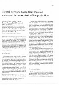
In this study, a neural network based scheme is applied to modify the reference trajectories of the joint angles of the two-link flexible robot manipulator depicted in figure 1, for the tracking control problem. The control scheme is shown in figure 2. The neural network operates online to calculate the incremental change in the command values of joint angles, while in the control loop a PD controller is applied to the manipulator. The reference trajectory for the joint angles can be decomposed into two parts:
θ ref = θ ref 1 + θ ref 2
W is the vector of neural network weights and ep denotes the error of the tip in the Cartesian coordinates. Separate neural networks are designed for each joint angle and they are composed of three layers; the input, hidden and output layer. Hyperbolic tangent functions are used as activation functions in the hidden layer, and linear functions are utilized in the output layer. An auxiliary variable, exy is defined to measure the error between the actual and desired positions of the tip of the robot manipulator.
exy =
(9)
In figure 2, p des denotes the desired trajectory for the tip of the manipulator in the operational space,
θ ref 1 is
calculated from p des using inverse kinematic equations of a two-link, planar rigid robot. θ ref 2 is calculated by the
(
)
ex xdes − x ep = p ref − p = = ey ydes − y
(
)
(12)
Error backpropagation method is used for training the neural networks and the weights are updated according to (13) in order to minimize the cost function given in (14).
neural network utilizing the information of error in the operational space.
θ ref 2 = NN W, ep
1 2 2 e + ey 2 x
∆W = −η
(10)
J=
∂J ∂W
(13)
1 2 e 2 xy
(14)
(11)
FIGURE 2. The control scheme
IV. PD CONTROLLER The incremental changes to be made in the reference values of the joint angles to minimize the tip error in Cartesian coordinates are calculated in the neural networks as described in section III, and added to the value obtained from inverse kinematic equations, hence the final value of the reference angles are obtained. In the control loop, a PD controller is utilized to obtain good tracking in the joint space. The actuator torques to be applied to each joint is given by:
~ ~• τ i = − k pi θ i ( t ) − k v i θ i ( t ) ~
(15)
~•
In equation (15), θ i ( t ) and θ i ( t ) represent the error in the joint angle and velocity for the ith link. k p and k v are i i the proportional and derivative gains, respectively. In the simulations, the controller gains are chosen as: k p = 5 , 1
k v1 = 3 , k p2 = 1.2 , kv2 = 0. 8 .
V.
SIMULATION RESULTS
0.02
0.01 0
-0.01
0
10
20 30 Time (sec)
40
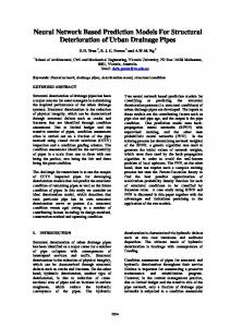
actual values of joint angles are depicted, figure 5 shows the deflection of each link. Figure 6 illustrates the comparison of the error of the tip of the manipulator in the operational space, with and without the incremental change calculated by the neural network. Similarly, figure 7 depicts the auxiliary variable exy, given by (14), and figure 8 shows the tip of the manipulator in the operational space, with and without the incremental change calculated by the neural network.
Modification on Elbow Angle (rad)
Modification on Shoulder Angle (rad)
Simulations are performed on the two-link, planar, flexible manipulator depicted in figure 1, to test the performance of the trajectory planning method described in section III and the PD controller explained in section IV. It is required that the tip of the manipulator tracks a rectangular trajectory in the operational space. Figures 38 illustrate the results of the simulations. In figure 3, the modification in reference joint angles obtained from neural networks are shown. In figure 4, the reference and
-4
6
x 10
4 2 0 -2
0
10
20 30 Time (sec)
40
FIGURE 3. The modification on reference values of joint angles calculated by neural networks
2.5 Elbow Angle (rad)
Shoulder Angle (rad)
2 1.5 1 0.5 0
0
10
20 30 Time (sec)
40
2
1.5
0
10
20 30 Time (sec)
FIGURE 4. Reference (dotted lines) and actual (solid lines) angles for the shoulder and elbow angles
40
-3
4 Defl. for Link 2 (m)
Defl. for Link 1 (m)
0.02 0.01 0 -0.01 -0.02
0
10
20 30 Time (sec)
2 0 -2 -4
40
x 10
0
10
20 30 Time (sec)
40
FIGURE 5. Deflection of the shoulder link and the elbow link 0.04 Error in y-direction (m)
Error in x-direction (m)
0.03 0.02 0.01 0 -0.01 -0.02
0
10
20 30 Time (sec)
40
0.02 0 -0.02 -0.04
0
10
20 30 Time (sec)
40
FIGURE 6. The errors in x- and y-coordinates of the tip of the manipulator in the operational space with (solid line) and without (dotted line)modification of reference joint angles -4
7
x 10
6
Auxiliary variable, exy
5
4
3
2
1
0
0
5
10
15
20 Time (sec)
25
30
35
40
FIGURE 7. The auxiliary variable exy with (solid line) and without (dotted line) modification of reference joint angles
0.3 0.2 0.1
y (m)
0 -0.1 -0.2 -0.3 -0.4 -0.5 0.35
0.4
0.45
0.5
0.55
0.6
0.65
0.7
x (m)
FIGURE 8. Desired trajectory (dash-dotted line) and the position of the tip of the manipulator in the operational space with (solid line) and without (dotted line) modification of reference joint angles
VI. CONCLUSIONS In this study, a neural network based trajectory planning method is applied to a planar, two-link flexible manipulator to provide a more precise tracking for the tip trajectory in the operational space. The reference values of joint angles are calculated by inverse kinematic equations of rigid manipulators. Then an incremental change for these joint angles is computed by a neural network which takes the errors in x- and y- coordinates of the tip in the operational space as inputs and updates its weights in order to minimize the error in the operational space. The incremental value is added to the reference value of the joint angle. In the control loop, the control of the joint angles is provided by a PD controller. As we can observe from the simulation results, in comparison to the case where there is no reference joint angle compensation for link flexibility, there is really a pronounced improvement in the operational space tracking performance of the tip of the manipulator. REFERENCES [1] De Luca A, Siciliano B, “Closed-Form Dynamic Model of Planar Multilink Leightweight Robots,” IEEE Transactions on Systems, Man and Cybernetics, Vol. 21, No. 4 s. 826-839, 1991. [2] Asada H, Ma ZD, Tokumaru H., “Inverse Dynamics of Flexible Robot Arms: Modelling and Computation for Trajectory Control,” ASME Journal of Dynamic Systems Measurement and Control, Vol. 112, s. 177-185, 1990.
[3] Bayo E, Papadopoulos P, Stubbe J, Serna MA “Inverse Dynamics and Kinematics of Multi-Link Elastic Robots: An Iterative Frequency Approach,” International Journal of Robotics Research, Vol. 8, No. 6, s. 49-62, 1989. [4] Sarkar PK, Yamamoto M, Mohri A, “On the Trajectory Planning of a Planar Elastic Manipulator Under Gravity,” IEEE Transactions on Robotics and Automation, Vol. 15, No. 2, s. 357-362, 1999. [5] Ubertini F, “A Contribution to the Analysis of Flexible Link Systems,” International Journal of Solids and Structures, Vol. 37, s.969-990, 2000. [6] Öke G, İstefanopulos Y, “Gradient-Descent Based Trajectory Planning for Regulation of a Two-Link Flexible Robotic Arm” 2001 IEEE/ASME International Conference on Advanced Intelligent Mechatronics, (AIM’01) Proceedings, Vol.II, s.948-952. [7] Rouvinen A, Handroos H, “Deflection Compensation of a Flexible Hydraulic Manipulator Utilizing Neural Networks,” Mechatronics, Vol. 7, No. 4, s. 355-368,1997. [8] Jung S., Hsia T.C., “Neural Network Inverse Control Techniques for PD Controlled Robot Manipulator”, Robotica, Vol.18, pp. 305-314, 2000.