neural network ensembles approach to address this problem using high ... In plug-level metering, a smart outlet monitors the real-time consumption of its ...
Neural Network Ensembles to Real-time Identification of Plug-level Appliance Measurements Karim Said Barsim, Lukas Mauch, and Bin Yang Institute of Signal Processing and System Theory, University of Stuttgart {karim.barsim,lukas.mauch,bin.yang}@iss.uni-stuttgart.de Abstract— The problem of identifying end-use electrical appliances from their individual consumption profiles, known as the appliance identification problem, is a primary stage in both NonIntrusive Load Monitoring (NILM) and automated plug-wise metering. Therefore, appliance identification has received dedicated studies with various electric appliance signatures, classification models, and evaluation datasets. In this paper, we propose a neural network ensembles approach to address this problem using high resolution measurements. The models are trained on the raw current and voltage waveforms, and thus, eliminating the need for well engineered appliance signatures. We evaluate the proposed model on a publicly available appliance dataset from 55 residential buildings, 11 appliance categories, and over 1000 measurements. We further study the stability of the trained models with respect to training dataset, sampling frequency, and variations in the steady-state operation of appliances. Index Terms— Plug-level monitoring, Distributed sensing, Neural network ensembles, PLAID dataset
I. I NTRODUCTION The energy end-use monitoring problem has received a widespread attention over the last two decades, either in a nonintrusive fashion using smart meters which aim at reducing the cost of installation and maintenance [1, 2] or distributed sensing and smart outlets that became available through recent technological developments [3, 4]. Both trends face what is referred to as the appliance identification problem. In nonintrusive monitoring, the disaggregation stage reconstructs endappliance consumption profiles from the aggregate measurements in a building. Afterwards, the appliance identification stage assigns either a generic end-use category [5] or specific appliance instances [6] to each reconstructed load profile. In plug-level metering, a smart outlet monitors the real-time consumption of its plugged-in appliance but this appliance may change over time based on user requirements. Similarly, identifying the connected appliance from the given consumption profile without user intervention is the challenge of appliance identification. Previous works have addressed the problem of appliance identification using various machine learning tools, electric signatures, or evaluation platforms. In [3] for instance, support vector machines (SVM) and decision trees (DTree) trained on three-month, second-based power profiles of over 20 appliances achieved comparable performance on future runs of the same appliances. The performance degraded notably as previously unseen appliances were added to the test. In [7], current harmonics in addition to a few more features were extracted from high-resolution current waveforms (during transient and steady-state operations) to compare various
classification algorithms. High accuracies were reported using Bayesian networks evaluated on 16 categories of appliances and over 3000 acquired measurements. A more recent study, and most related to this work, compared and evaluated nine classifiers (including kNNs, logistic regression, SVMs, and DTrees) on different raw and engineered features [4] from a publicly available power dataset [8]. The authors proposed a novel appliance signature based on quantization of the VItrajectories into a binary VI-image. The study further examined the effect of the sampling frequency on the identification problem showing that high classification rates can be obtained using random forest trees trained on the raw current and voltage measurement of at least 4kHz of sampling frequency (up to 82% of accuracy using VI-images and 86% using a set of combined features). In most of these works neural networks on raw measurements have received little or no attention as a candidate model for appliance identification. Neural networks have recently received a growing interest in various machine learning applications especially after the evaluation of a deep convolutional architecture on a visual recognition dataset known as ImageNet. Recently, different deep learning architectures were found to achieve comparable results in the problem of energy disaggregation [9, 10]. In this paper, we first complement the work in [4] with an ensemble of neural networks in addressing the appliance identification problem from the raw, high-resolution current and voltage waveforms. We further study the stability and robustness of the proposed model with respect to the size of the training dataset, the sampling frequency of the measurements, and signal variations during the steady-state operation of appliances. We evaluate our models on the publicly available plug load appliance identification dataset (PLAID) [8] which contains, at the time of this work, measurements from 11 appliance categories, 235 appliance instances distributed over 55 households, and a total of 1074 current and voltage measurements at a sampling frequency fs = 30kHz and a grid frequency fg = 60Hz. II. A PPLIANCES ’ SIGNATURES In this work, we utilize the raw current i(n) and voltage v(n) waveforms during the steady-state operation as an appliance signature. Unlike previous works on VI-trajectories that extracted shape-based features [11, 12], we exploit one of the advantages of neural nets by utilizing the raw signals directly. Given current i(n) and voltage v(n) signals of an appliance at a sampling frequency fs and a grid frequency fg , we extract
one complete period of each waveform � �T ϕτ = ϕ(τ ), ϕ(τ +1), . . . , ϕ(τ +d-1) ∈ Rd , ϕ ∈ {i, v}
where d = fs /fg is the number of samples per period and τ is a point in time during the steady-state operation of the appliance. In order to support category-based appliance identification, we alleviate all amplitude information through segment-based normalization where each extracted signal segment ϕτ is normalized to the range [-1,1]. The result is the signal segments � 2ϕτ − max ϕτ + min ϕτ Jd,1 � ˆτ = ϕ ∈ [−1, 1]d (1) max ϕτ − min ϕτ where Jm,n is an m-by-n matrix of ones. The input vector to the neural network hbecomes i T x = ˆiT , vˆT ∈ [−1, 1]2d (2) τ
τ
which corresponds to an input layer of size 2d for each neural network. We further expand the size of the training set algorithmically through extracting several signal segments from equally spaced initial phases of each measurement � � d X = xτ τ = τo +i ε , 0 ≤ i < (3) ε where ε is the sliding step of the extraction window and this is applied to each measurement. Algorithmic expansion of the training data has several advantages. It provides a larger set of training data, eliminates the need for phase alignment of the signals, and more importantly drives a fully connected neural network to become invariant to the initial phase of the extracted signals. As a result, the model becomes more robust to signal variations during steady-state operation of appliances.
III. P REDICTION MODEL Given a set Ω = {ωm }M m=1 of M class labels (i.e. appliance categories), the straightforward approach for appliance classification is a multi-class neural network. However, in our initial tests we observed that an ensemble of binary networks performs consistently better than the multi-class model with a similar total size (i.e. neurons), training algorithm, regularization method, and overall training time. It is known that neural networks are one of the unstable learning algorithms with respect to training data [13] (i.e. they are sensitive to changes in the training set). For unstable models, an ensemble approach known as Bootstrap aggregation (aka Bagging) [14, 15] is expected to provide better results than a single base model1. We, therefore, adopt the latter approach (i.e. an ensemble of binary networks) and discuss it further in the following. For each class combination (ωi , ωj )i pˆωj ,ωi (x) ωi ∈ Ω
(8)
j6=i
for unweighted majority voting where 1 is the indicator function. Finally, we utilize a validation-based early stopping as a regularization technique to avoid over fitting [16]. As mentioned earlier, PLAID measurements contains, for each appliance category, several appliance instances from various households. In order to improve generalization ability to new buildings, a 30% validation set is selected in a building-based fashion. IV. E VALUATION We evaluate our models on the publicly available PLAID dataset [8] which contains � M = 11 appliance categories. Therefore, we have M = 55 class combinations and for 2 each we train a two-layer, fully connected, feed-forward neural network with 2d input neurons, 30 hidden neurons, and two output neurons. Since some measurements contain turnon transients, which are to be avoided in this work, the training set is extracted from the last two periods of each measurement. With a sliding step of ε = 10 samples, the training dataset is expanded by a factor of d/ε = 50. The hyperbolic tangent (tanh) activation is utilized in the hidden layer while the normalized exponential (softmax) is selected for the output layer. We utilized matlab’s implementation of the conjugate gradient descent with random restarts [17] as a training function for all models. In order to compare this approach with the previously studied models on this dataset [4], we adopt the same leavehouse-out cross validation technique. In other words, samples from one house is saved for test while the remaining set of buildings are available for training, resulting in a total of 55 test cases. For each class ωm and the total confusion matrix Λ = [Λij ]M i,j=1 , we introduce the following performance indicators n ˜ ω TPm = x ∈ X ˆ (x) = ωm n ˜ ω TNm = x ∈ X ˆ (x) 6= ωm n ˜ ω FPm = x ∈ X ˆ (x) = ωm n ˜ ω FNm = x ∈ X ˆ (x) 6= ωm
o & ω(x) = ωm o & ω(x) 6= ωm o & ω(x) 6= ωm o & ω(x) = ωm
(9) (10) (11) (12)
VI-Trajectories
1 AC 1-1 CFL 1-1 Fan 1-1
-1 Voltage
1-1 Hairdryer 1-1 Fridge
0
2
4
6
8
10
0.5
0.926 0.980 0.893 0.962 0
0.5
0.774 0.997 0.889 0.686 0
0.5
0.882 0.976 0.824 0.947 0
0.5
1
F1S TNR PPV TPR
0.956 0.994 0.970 0.942 0
0.5
1
F1S TNR PPV TPR
0.986 0.999 0.993 0.978 0
0.5
1
F1S TNR PPV TPR
0.961 0.998 0.949 0.974 0
0.5
1
F1S TNR PPV TPR
0.894 1.000 1.000 0.808 0
0.5
1
0.0
0.0
0.0
0.0
0.0
0.0
0.0
0.0
0.0
0.0
1.0
0.5
0.5
0.5
0.0
0.0
0.0
0.0
0.0
0.0
0.0
0.0
0.0
0.0
0.0
0.0
0.0
0.0
0.0
0.0
κ α
0.5
κ α
0.5
κ α
0.5
κ α
0.5
κ α
0.5
κ α
0.5
κ α
0.5
κ α
0.5
κ α
0.5
κ α
0.5
κ α
0.5
κ
0.0 1.0
0.74 0.80
0.88 0.90
0.0 1.0
0.5
Total
1.0
0.5
1.0
1.0
0.5
0.0
κ α
0.0
1.0
0.5
House 55
0.0
1.0
1.0
0.64 0.71
0.0
1.0
0.5
1.0
κ α
0.0
1.0
1.0
0.77 0.81
0.0
0.5
0.80
0.0 1.0
1.0
—–
0.5
1.00 1.00
0.5
1.00 1.00
0.5
0.91 0.94
1.0
0.5
1.00 1.00
0.0 1.0
1.0
0.5
1.00 1.00
1.0
1.0
0.5
1.00 1.00
0.0
1.0
1.00
0.0
—–
0.0
0.5
1.00
0.5
1.0
House 19
0.0
1.0
House 38
0.0
1.0
1.00 1.00
0.0
1.0
1.00
0.0
1.0
—–
0.0
1.00
0.0 1.0
—–
0.5
0.74 0.77
0.5
0.66 0.71
0.5
0.66 0.72
0.5
1.00 1.00
0.5
0.67 0.75
0.5
1.00 1.00
0.5
1.00 1.00
0.5
0.80 0.85
0.5
1.00
0.5
—–
0.5
1.00 1.00
1.0
α
1.0
1.00 1.00
1.0
1.00 1.00
1.0
0.68 0.86
1.0
0.81 0.85
1.0
0.75 0.80
1.0
0.69 0.75
1.0
1.00 1.00
1.0
1.00 1.00
1.0
0.76 0.79
0.84 0.87
1.0
0.5
0.5
κ α
1
F1S TNR PPV TPR
0.5
κ α
1
F1S TNR PPV TPR
0.5
κ α
1
Time [ms]
1.00 1.00
0.82 0.85
0.79 0.83
0.740 0.992 0.771 0.711
0.5
0.5
1.0
1.0
1
0.5
0.85 0.89
1.00
—–
0.69 0.75
1.0
—–
0.0 1.0
1.0
0.85 0.87
1.0
1.00
0.0
—–
0.0
0.5
1.0
1.00 1.00
0.90 0.92
0.0
1.0
0.95 0.96
0.0
0.5
1.0
0.93 0.95
0.0 1.0
0.73 0.79
0.5
0.50
0.90 0.92
0.5
0.5
1.00 1.00
0.96 0.97
House 20
0.92 0.93
0.0 1.0
1.0
0.5
—–
1.00 1.00
0.90 0.93
House 1
0.5
1.0
12
1
14
-1
16
Current
16
14
12
10
8
6
4
2
-1 1
0.5
F1S TNR PPV TPR
Bulb 2
4
6
8
10
12
1
14
-1
16
Current
16
14
12
10
8
6
4
2
-1 1
1
0.741 0.985 0.844 0.661 0
1-1 Vacuum 1-1Microwave 1-1 Laptop 1-1
2
4
6
8
10
12
1
14
-1
16
Current
16
14
12
10
8
6
4
2
-1 1
0.5
F1S TNR PPV TPR
-1 W. M.
2
4
6
8
10
12
1
14
-1
16
Current
16
14
12
10
8
6
4
2
-1 1
1
0.969 0.993 0.966 0.971 0
2
4
6
8
10
12
1
14
-1
16
16
14
12
10
8
6
4
2
Current
-1 1
0.5
F1S TNR PPV TPR
1-1 Heater
2 2 2
4
6
8
10
12
1
14
-1
16
Current
16
14
12
10
8
6
4
2
-1 1
1.0
0
2
4
6 6
4 4
6
8
10
12
1
14
-1
16
Current
16
14
12
10
8
6
4
2
-1 1
0.698 0.969 0.627 0.788
F1S TNR PPV TPR
2
4
6
8
10 10
8 8
10
12
1
14
-1
16
Current
16
14
12
10
8
6
4
2
-1 1
1.0
Performance F1S TNR PPV TPR
2
4
6
8
10
14
12 12 12
1
14
-1
16
Current
16
14
12
10
8
6
4
2
Fan
-1 1
1-1 1-1 Hairdryer 1-1 Fridge 1-1 Heater
14
1
16
Current
16
14
12
10
8
6
4
-1
1-1
2
CFL
-1 1
Bulb 1-1 Vacuum 1-1Microwave 1-1 Laptop 1-1 -1 W. M.
16
Current
16
14
12
8
10
6
4
2
1
1-1
-1
Time [ms]
House 39
Voltage
1
AC
1
Current
Fig. 1: Current, voltage, and VI-trajectories of selected samples from PLAID dataset [8] are shown to the left. The appliance categories and IDs, from top to bottom, are (1) air conditioner, 1010, (2) CFL, 20, (3) fan, 766, (4) fridge, 6, (5) hairdryer, 444, (6) heater, 716, (7) bulb, 57, (8) laptop 28, (9) microwave, 10, (10) vacuum cleaner, 730, and (11) washing machine, 488. The per-category evaluation metrics are shown to the right while the per-house metrics are in the bottom. The best evaluation results are κ = 0.882 and α = 0.897.
1.0 0.9 0.8 0.7 0.6
0.1
0.2
0.3
0.4
0.5
0.6
0.7
0.8
0.9
1.0 0.1
0.2
0.3
0.4
Size of training set r
0.5
0.6
0.7
0.8
0.9
1.0
0.9 0.7
0.8
0.9 0.8
Cohen’s κ
1.0
1.0
Size of training set r
0.7
10
15
20
25
30
5
10
15
20
25
30
Sampling frequency fs [kHz]
0.8
0.8
0.9
0.9
1.0
1.0
Sampling frequency fs [kHz]
0
0.1
0.2
0.3
0.4
0.5
0.6
0.7
0.8
0.9
0
0.1
0.2
0.3
0.4
0.5
0.6
0.7
0.8
Cohen’s κ
Accuracy α
5
Accuracy α
Cohen’s κ
1.0 0.9 0.8 0.7 0.6
Accuracy α
ˆh Reduced label space Ω
Complete label space Ω
0.9
Time τ [s] Time τ [s] Fig. 2: Aggregate evaluation results as a function of (a) training set size, (b) sampling frequency, and (c) time shift. To right are the same experiments with reduced label spaces based on the prior knowledge of the label space of each target household.
recallm = TPRm = TPm / (TPm + FNm ) precisionm = PPVm = TPm / (TPm + FPm ) specificitym = TNRm = TNm / (TNm + FPm ) 2TPm Fm 1 -score = F1Sm = 2TPm + FPm + FNm
(13) (14) (15) (16)
for per-class evaluation whereas the unweighted accuracy α and Cohen’s κ tr(Λ) tr(Λ) = , α = PM J 1,M ΛJM,1 i,j=1 Λi,j κ=
tr(Λ) × J1,M ΛJM,1 − tr ΛJM Λ �2 � J1,M ΛJM,1 − tr ΛJM Λ
(17) �
(18)
are utilized for the aggregate, multi-class evaluation. Figure 1 shows the per-class, and per-household performance results. The best result obtained for the voting in Equation 7 is α = 89.7% while the unweighted majority vote Equation 8 achieved 88.2% of accuracy. It is observed from the figures that microwaves, compact fluorescent lamps, vacuum cleaners, and laptops are the most identifiable loads whereas temperature control devices (such as air conditioners, heaters, fridges, and even fans) are the least. Figure 2 shows further tests of stability of the adopted model. In the first study, we reduce the size of the training dataset and estimate the total performance using the same cross validation technique. In each test case, one building is saved for evaluation, 54r buildings for training where 0 < r ≤ 1 (which is further partitioned into training and validation households), and the remaining 54(1 − r) are untouched. As expected, the performance of the model degrades notably as the size of the training data decreases. In the second study, we use the complete training dataset (i.e. r = 1) but reduce the sampling frequency of the raw mea-
surements. A suitable FIR filter is utilized for each fractional decimation. This study reveals the robustness of our method with respect to the sampling frequency. As observed in the figure, the accuracy slightly drops but is always above 80% even at 2.5kHz. In the third study, we test the sensitivity of the model to the phase shift of the extracted segments. In other words, a single period from each measurement with phase τ is extracted for testing. The common shortest period of all PLAID measurements is one second. Similarly, the figure reveals the robustness of the proposed model to signal variations in steadystate operation, at least for the short common period available in PLAID. Finally, we repeat all previous experiments while exploiting external knowledge about the list of appliances in each house in reducing the label space for each test case. In other words, if house h = 1 does not have an air conditioner, the label ˜ 1 = Ω − {'AC'} and we space for this building becomes Ω rather train 45 binary networks. This of course improves the performance where the best-case accuracy reaches α = 94%, but the question is of course about the availability of this knowledge in practice. V. C ONCLUSION AND FUTURE WORK In this work, we introduced an approach of ensemble of neural networks in addressing the appliance identification problem using raw, high-resolution current and voltage measurements. We evaluated our model on the PLAID dataset with the best performance test achieving 89% of accuracy. It was observed that the performance notably degrades as the size of the training data is reduced. Therefore, one of the main future work packages is semi-supervised learning methods.
R EFERENCES [1] G. W. Hart, “Nonintrusive appliance load monitoring”. In proceedings of the IEEE 80 (12):1870–1891, Dec. 1992. [2] J. Froehlich, E. Larson, S. Gupta, G. Cohn, M. S. Reynolds, and S. N. Patel, “Disaggregated End-Use Energy Sensing for the Smart Grid”. In proceedings of Pervasive Computing, IEEE 10 (1):28–39, Jan. 2011. [3] S. Barker, M. Musthag, D. Irwin, and P. Shenoy, “NonIntrusive Load Identification for Smart Outlets”. In proceedings of the IEEE International Conference on Smart Grid Communications (SmartGridComm):548–553, Nov. 2014. [4] J. Gao, E. C. Kara, S. Giri, and M. Berg´es, “A feasibility study of automated plug-load identification from highfrequency measurements”. In proceedings of the 3rd IEEE Global Conference on Signal and Information Processing (GlobalSIP):220–224, Dec. 2015. [5] O. Parson, S. Ghosh, M. Weal, and A. Rogers, “An Unsupervised Training Method for Non-intrusive Appliance Load Monitoring”. Artificial Intelligence 217:1–19, 2014. [6] J. Z. Kolter and T. Jaakkola, “Approximate Inference in Additive Factorial HMMs with Application to Energy Disaggregation”. In proceedings of the International Conference on Artificial Intelligence and Statistics 22:1472– 1482, 2012. [7] A. Reinhardt, D. Burkhardt, M. Zaheer, and R. Steinmetz, “Electric Appliance Classification Based on Distributed High Resolution Current Sensing”. In proceedings of the 37th IEEE Conference on Local Computer Networks (LCN):999–1005, Oct. 2012. [8] J. Gao, S. Giri, E. C. Kara, and M. Berg´es, “PLAID: A Public Dataset of High-resolution Electrical Appliance Measurements for Load Identification Research: Demo Abstract”. In proceedings of the 1st ACM Conference on Embedded Systems for Energy-Efficient Buildings:198– 199, 2014. [9] J. Kelly and W. J. Knottenbelt, “Neural NILM: Deep Neural Networks Applied to Energy Disaggregation”. CoRR abs/1507.06594 , Aug. 2015. [Online]. Available: http://arxiv.org/abs/1507.06594 [10] L. Mauch and B. Yang, “A new approach for supervised power disaggregation by using a deep recurrent LSTM network”. In proceedings of the 3rd IEEE Global Conference on Signal and Information Processing (GlobalSIP):63–67, Dec. 2015. [11] H. Y. Lam, G. Fung, and W. K. Lee, “A Novel Method to Construct Taxonomy Electrical Appliances Based on Load Signaturesof”. Consumer Electronics, IEEE Transactions on 53 (2):653–660, May 2007. [12] T. Hassan, F. Javed, and N. Arshad, “An Empirical Investigation of V-I Trajectory Based Load Signatures for Non-Intrusive Load Monitoring”. IEEE Transactions on Smart Grid 5 (2):870–878, Mar. 2014. [13] C. C. Aggarwal, Data Classification Alrogithms and Applications. Chapman & Hall/CRC, 2015. [14] L. Breiman, “Bagging Predictors”. Machine Learning 24
(2):123–140, 1996. [15] J. H. Friedman and P. Hall, “On bagging and nonlinear estimation”. Journal of Statistical Planning and Inference 137 (3):669 – 683, 2007. [16] L. Prechelt, “Early Stopping - but when?”. Neural Networks: Tricks of the Trade:53–67, 2012. [17] M. J. D. Powell, “Restart procedures for the conjugate gradient method”. Mathematical Programming 12 (1):241–254, 1977.