Neural network firing-rate models on integral form - CiteSeerX

Biological Cybernetics manuscript No. (will be inserted by the editor)

Øyvind Nordbø · John Wyller · Gaute T. Einevoll

Neural network firing-rate models on integral form Effects of temporal coupling kernels on equilibrium-state stability

Received: date / Accepted: date

Abstract Firing-rate models describing neural network activity can be formulated in terms of differential equations for the synaptic drive from neurons. Such models are typically derived from more general models based on Volterra integral equations assuming exponentially decaying temporal coupling kernels describing the coupling of pre- and postsynaptic activities. Here we study models with other choices of temporal coupling kernels. In particular, we investigate the stability properties of constant solutions of two-population Volterra models by studying the equilibrium solutions of the corresponding autonomous dynamical systems, derived using the linear chain trick, by means of the Routh-Hurwitz criterion. In the four investigated synaptic-drive models with identical equilibrium points we find that the choice of temporal coupling kernels significantly affects the equilibriumpoint stability properties. A model with an α-function replacing the standard exponentially decaying function in the inhibitory coupling kernel is in most of our examples Ø. Nordbø Department of Mathematical Sciences and Technology and Center for Integrative Genetics, Norwegian University of Life Sciences, P.O.Box 5003, 1432 ˚ As, Norway Tel.: +47-73593955 Fax: +47-73592889 E-mail: [email protected] Present address: SINTEF Energy Research, 7465 Trondheim, Norway J. Wyller Department of Mathematical Sciences and Technology and Center for Integrative Genetics, Norwegian University of Life Sciences, P.O.Box 5003, 1432 ˚ As, Norway Tel.: +47-64965489 Fax: +47-64965401 E-mail: [email protected] G.T. Einevoll Department of Mathematical Sciences and Technology and Center for Integrative Genetics, Norwegian University of Life Sciences, P.O.Box 5003, 1432 ˚ As, Norway Tel.: +47-64965433 Fax: +47-64965401 E-mail: [email protected]

found to be most prone to instability, while the opposite situation with an α-function describing the excitatory kernel is found to be least prone instability. The standard model with exponentially decaying coupling kernels is typically found to be an intermediate case. We further find that stability is promoted by increasing the weight of self-inhibition or shortening the time constant of the inhibition. Keywords neural networks · firing rate · Volterra · stability · temporal coupling · Routh-Hurwitz

1 Introduction Following pioneering work of, e.g., Wilson and Cowan (1973) and Amari (1977) in the 1970’s, a tradition has developed for studying simplified cortical-network models using field descriptions. In this approach the individual times for firing of action-potentials are not modeled, only the firing rate, that is, the probability densities for firing. Likewise, a continuum description of the set of neurons constituting the neural network is typically used so that the neural firing activities can be described by scalar fields in terms of a time and one or two space coordinates. Neural field models have been widely used to investigate generic features such as the generation and/or stability of coherent structures such as spatially localized bumps, spatially or spatiotemporally oscillating patterns, and travelling waves, pulses and fronts. For reviews of the comprehensive literature, see Ermentrout (1998), Bressloff (2005), Coombes (2005) and Vogels et al. (2005). Existing firing-rate models are typically formulated in terms of sets of ordinary differential equations. For synaptic-drive models (Pinto et al. 1996; Ermentrout 1998) each ordinary differential equation has the form τj

³X ´ duj + uj = gj wjk uk dt j

(1)

2

Nordbø, Wyller, Einevoll

where a physiological interpretation is that uj is the the exponential kernel, i.e., α-functions (∼ t exp(−t/τ ), ’synaptic drive’ from neural element j (Pinto et al. 1996), t > 0) which has its maximum at time t = τ . This τj is a time constant reflecting the decay of this synap- function is commonly used to model synaptic currents tic drive following an action-potential in element j, and and conductances, see, e.g., Ch. 5 in Dayan and Abbott wjk is the synaptic weight from element k onto element (2001). α-function temporal coupling kernels have also j. gj (x) is the firing-rate function of neural element j, been used in previous investigations of stability properconverting the net synaptic drive onto element j into a ties of such background states in other neural network firing rate. This function is typically assumed to have a models (Hutt et al. 2003; Hutt and Atay 2005; Atay and sigmoidal form. Hutt 2006). The firing-rate model in (1) can be derived from Volterra In the analysis we employ the ’linear chain trick’ integral-equation models with exponentially decaying tem- (Cushing 1977), previously used in a neural network conporal coupling kernels (Ermentrout 1998; Dayan and Ab- text by, e.g., Laing and Longtin (2003), to reformulate bott 2001). The dynamics described by (1) corresponds the Volterra systems as sets of coupled differential equations which are then analyzed by means of dynamical to ³X ´ systems theory. In particular, we investigate the stability uj (t) = hj (t) ∗ gj wjk uk (t) , where (2) of the equilibrium point by means of the Routh-Hurwitz j criterion and use Hopf’s theorem to investigate the ex1 −t/τj istence of generic Hopf bifurcations as stability is lost hj (t) = e (3) (Ermentrout and Cowan 1979a). τj and the ’asterisk’ denotes a temporal convolution. The form of (2) clarifies the above physiological interpretation of the temporal coupling kernel hj (t): it describes the temporal form of the ’synaptic drive’ uj following firing of an action potential in element j as felt in the soma of its postsynaptic neurons. This temporal form will reflect the temporal form of the synaptic current (i.e., the type of postsynaptic receptors), the distance from the synapse to the soma of the postsynaptic neuron, as well as electrical properties of the postsynaptic dendrites. While the assumption of an exponentially decaying temporal kernel may be reasonable in some situations, it is also clear that this cannot generally be the case. For example, a synaptic input current with an exponentially decaying temporal shape onto a distal part of an apical dendrite of a large layer-5 pyramidal neuron, will not result in an instantaneous and exponentially decaying disturbance of the somatic potential: while the disturbance will be initiated immediately, the maximum disturbance will come some time later. Even a synaptic input at a fast AMPA synapse at the basal dendrites appears to give an EPSP at the soma that resembles an αfunction more than a decaying exponential (see Fig. 18.1 in Koch (1999)). In the present study we investigate stability properties of equilibrium states in firing-rate models of the type in (2) with various types of temporal coupling kernels hj (t). This issue of the properties of the background state is getting more important as one starts to explore network models where the dynamics is determined by a combination of the background state and stimulusevoked input (Vogels et al. 2005). The common choice of studying rate models of the type in (1), mainly motivated by mathematical convenience, implicitly corresponds to assuming exponentially decaying temporal kernels (3). Here we consider two-population models (excitatory+inhibitory) and, in particular, investigate the consequences of choosing other temporal kernels than

2 Generalization of firing-rate model We consider a two-population (excitatory+inhibitory) synaptic-drive model where the starting point is the following Volterra equation system, ue = he ∗ ge (wee ue − wei ui ) ui = hi ∗ gi (wie ue − wii ui )

(4) (5)

where ue (ui ) denote the excitatory (inhibitory) ’synaptic drive’. gn is the firing-rate function modelled by means of a piecewise linear function (Tsodyks et al. 1997; Koch 1999; Tateno et al. 2004),   xn < θ n 0 , gn (xn ) = βn (xn − θn ) , θn ≤ xn ≤ θn + 1/βn (n = e, i)  1 , xn ≥ θn + 1/βn (6) The time history of the network is given by the convolution integral hn ∗ gn , (n = e, i) defined as Z t ¡ ¢ hn (t − s)gn (xn (s))ds (7) hn ∗ gn (xn ) (t) ≡ −∞

The non-negative parameters wmn , m, n = e, i, represent the synaptic weights, and θn , n = e, i, is the activity threshold for firing for the excitatory and inhibitory populations. βn measures the steepness of the firing-rate function. RFinally, the temporal kernels hn are normal∞ ized, i.e., 0 hn (t)dt = 1, continuous and bounded. First, notice that the following properties hold true independent of the specific choice of temporal kernels: – Since gn , n = e, i, is Lipschitz continuous and bounded and the h-kernels are continuous and bounded, we know, according to Appendix A, that the system will be globally well-posed.

Neural network firing-rate models on integral form

3

– The scaling transformation (8)

shows that we may put the scaling parameter to βn = 1 without loss of generality. In what follows we assume βn = 1 and drop the tilde notation. – The constant solutions of (4)-(5) are independent of the temporal kernels h. For the oblique part of the firing-rate function, i.e., when θn < xn < θn + 1, the coordinates of these solutions (ue , ui ) ≡ (ue (0) , ui (0) ) are given as (Tsodyks et al. 1997) wei θi − (1 + wii )θe wei wie + (1 − wee )(1 + wii ) (wee − 1)θi − wie θe = wei wie + (1 − wee )(1 + wii )

ue (0) = ui (0)

(9) (10)

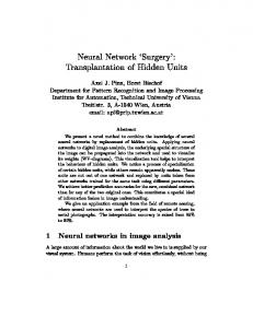
Moreover since 0 ≤ gn (x) ≤ 1, it follows from the system (4)-(5) that 0 ≤ un ≤ 1 (where n = e, i). From the expressions (9)-(10) we see that the latter condition imposes the conditions (i) sgn[N ]=sgn[D], and (ii) |D| > |N |, where D and N denote the denominator and numerator. In what follows we will investigate the equilibrium states, i.e., the constant solutions, and their stability properties for the model (4)-(5) using the standard exponentially decaying coupling kernels as well as three model variations with different choices of temporal coupling kernels for the excitatory (he (t)) and inhibitory populations (hi (t)). To be specific, we consider 1 −t/τ e (11) τ t Model A: he (t) = e−t , hi (t) = 2 e−t/τ (12) τ 1 (13) Model B: he (t) = t e−t , hi (t) = e−t/τ τ t Model C: he (t) = t e−t , hi (t) = 2 e−t/τ (14) τ for t ≥ 0. All kernels are causal, i.e., h(t < 0) = 0. Note that the time constant of the excitatory coupling kernel in all cases is set to unity (without loss of generality), and the inhibitory kernel time constant τ is thus measured in units of this excitatory kernel time constant. In Fig. 1 we illustrate the forms of the two types of temporal kernels considered: the exponentially decaying kernel (∼ exp(−t/τ )) and the α-function kernel (∼ t exp(−t/τ )). By using the linear chain trick (Cushing 1977) as described in detail in Appendix A, we derive autonomous dynamical systems governing the time evolution of smooth solutions of the system (4)-(5) for the four choices of temporal kernels listed above. The constant solutions (9)-(10) can be expressed in terms of the equilibrium points of the corresponding dynamical systems. Thus the stability properties of the constant solutions of (4)-(5) can be translated into stability properties of the corresponding equilibrium points. It should be noted that Standard: he (t) = e−t , hi (t) =

0.8

h(t)/h(0)

−1 wmn = βm w emn , θn = βn−1 θen

1

0.6

0.4

0.2

0 0

1

2

3

4

5

t

Fig. 1 Illustration of temporal kernels considered. Solid ¡ line: exponentially decaying h(t) = exp(−t/τ )H(t)/τ ; H(t) ¢ is Heaviside unit step function. . Dashed line: α-function ¡ ¢ h(t) = t exp(−t/τ )H(t)/τ 2 . τ = 1.

the stability properties of the equilibrium points in general turn out to be determined by only four parameters: τ , wee , wii , and the product wei wei . Here we will consider two special situations with a restricted parameter space in detail: (i) All synaptic weights are equal (w = wee = wei = wie = wii ), i.e., two freely varying parameters τ and w. (ii) Self-excitation is equal to one (wee = 1), i.e., three freely varying parameters τ , wii , and wei wei . 2.1 Standard temporal coupling kernel We first review the properties of the standard two-population firing-rate model corresponding to the temporal kernels in (11). With our choice of a piecewise linear firing-rate function (6) this corresponds to the system studied by Tsodyks et al. (1997). The Volterra equation system (4)(5) can in this case be converted to a 2D autonomous dynamical system by means of the linear chain trick (Cushing 1977): u0e = −ue + ge (wee ue − wei ui ) τ u0i = −ui + gi (wie ue − wii ui )

(15) (16)

As noted above, τ is the ratio between the inhibitory and the excitatory timescales. Since the firing-rate function is a piecewise linear function, the system (15)-(16) is a linear system on each of the linear segments. Let us consider the part of this system for which 0 < un < 1, n = e, i. The Jacobian of the RHS of (15)-(16) is in this case given as · ¸ wee − 1 −wei Js = (17) wie /τ −(1 + wii )/τ Since the system (15)-(16) is a 2D system, the stability issue of the equilibrium points given by (9) and (10) can

4

Nordbø, Wyller, Einevoll

be completely resolved by means of the invariants of the Jacobian, i.e., by means of the trace and the determinant: tr[Js ] = wee − 1 − (1 + wii )/τ det[Js ] = (1 + wii − wee + wei wie − wee wii )/τ

(18) (19)

from which it follows that stability is obtained provided wee − 1 − (1 + wii )/τ < 0, 1 + wii − wee + wei wie − wee wii > 0

and

(20) (21)

In the complementary regime the equilibrium is unstable. Now, let us consider our two special cases: (i) when w = wee = wei = wie = wii we get stability for 0 < τ ≤ 1, w > 0 and τ > 1, w < wsH (τ ) where wsH (τ ) = (τ + 1)/(τ − 1)

(22)

Moreover, the theory elaborated in Appendix B shows that the curve τ > 1, w = wsH (τ ) represents a Hopf bifurcation. It should be noted that Hopf’s theorem also applies in the present situation despite the choice of a piecewise linear firing-rate function (6). This theorem presupposes that the vector field defining the dynamical system is at least three times continuously differentiable in an open simple connected subset about the equilibrium point (Perko 2000). This means that in the present situation where the equilibrium points occur at the oblique part of the firing-rate functions, Hopf’s theorem is applicable. (ii) When wee = 1, we have tr[Js ] < 0 and det[Js ] > 0 for the whole parameter space from which it follows we we always have stability.

The characteristic equation P3 (λ) of this matrix is given as P3 (λ) = λ3 + a1 λ2 + a2 λ + a3

(28)

where the coefficients are given by: a1 = 2/τ − wee + 1 a2 = (2τ − 2wee τ + wii + 1)/τ 2 a3 = (1 − wii wee + (wii − wee ) + wei wie )/τ 2

The Routh-Hurwitz criterion presented in Appendix B is now used to determine the stability properties. For our first special case, w = wee = wei = wie = wii , we find after some algebra that the region in parameter space predicting stable equilibria will be bounded from above by wAH (τ ), where wAH (τ ) =

2(τ + 1)2 √ 2τ 2 + 2τ − 1 + 2τ 3 − 2τ + 1

The first variation we consider to the standard model is a model where the exponentially decaying temporal kernel of the inhibitory population hi (t) is replaced by an α-function (12). As shown in Appendix A, for this model the linear chain trick produces the following 3D autonomous system, u0e = −ue + ge (wee ue − wei ui ) τ u0i = −ui + yi τ yi0 = −yi + gi (wie ue − wii ui )

(23) (24) (25)

for the time evolution of the synaptic drives. Here yi is an auxiliary variable defined as Z ¢ 1 t −(t−s)/τ ¡ yi (t) = e gi wie ue (s) − wii ui (s) ds (26) τ −∞ The Jacobian J of the system (23)-(25) evaluated at the equilibrium point of this system is given as   wee − 1 −wei 0 −1/τ 1/τ  J= 0 (27) wie /τ −wii /τ −1/τ

(32)

We now use the synaptic weight as a control parameter and investigate the transversality conditions by means of the theory worked out in Appendix B.2. We find that two eigenvalues cross the imaginary eigenvalue axis transversally when w = wAH (τ ), and that the remaining eigenvalue is nonzero. Hence we can conclude that the threshold function wAH (τ ) represents a generic Hopf bifurcation in this model. For our second special case, wee = 1, we find that the equilibrium is stable if and only if η < ηAH (τ, wii ), where η is given as the product of the cross-connection synaptic weights (η = wei wie ), and ηAH (τ, wii ) = 2(1 + wii )/τ

2.2 Model A

(29) (30) (31)

(33)

We now use η as control parameter and find that the curve ηAH (τ, wii ) corresponds to a transversal crossing of the imaginary eigenvalue axis, and that the remaining eigenvalue is nonzero. Hence we can conclude that the threshold value ηAH (τ, wii ) also corresponds to a generic Hopf bifurcation. 2.3 Model B We now investigate the analogous model where the αfunction integral kernel is assumed for the excitatory population while the inhibitory kernel is modelled as a decaying exponential (13). The corresponding dynamic system can be obtained directly from the model-A equation set in (23)-(25) by the transformation ue −→ ui , ui −→ ue , yi −→ ye , θe −→ θi , θi −→ θe (34) and the parameter transformation wee −→ −wii , wie −→ −wei ,

−wei −→ wie −wii −→ wee ,

τ −1 −→ τ

(35)

Neural network firing-rate models on integral form

5

trick converts the Volterra system to the 4D autonomous dynamical system

7 wsH wAH

6

u0e τ u0i ye0 τ yi0

w

BH

wCH

5

w

4

= −ue + ye = −ui + yi = −ye + ge (wee ue − wei ui ) = −yi + gi (wie ue − wii ui )

where the pair of auxiliary variables (ye , yi ) are defined as Z t ¡ ¢ ye (t) = e−(t−s) ge wee ue (s) − wei ui (s) ds (42)

3 2

−∞ Z t

1 0 0

(38) (39) (40) (41)

1

2

3

τ

4

5

6

7

Fig. 2 Curves separating parameter regimes predicting stable (below curves) and unstable equilibria (above curves) for our four models when synaptic weights are equal, i.e., w = wee = wei = wie = wii . Solid line: standard model, wsH (τ ) (22). Dashed line: model A, wAH (τ ) (32). Dash-dotted line: model B, wBH (τ ) (36). Dotted line: model C, wCH (τ ) (50). The open dot corresponds to the point τ = 4, w = 1.1 while solid dot corresponds to the point τ = 4, w = 1.3, cf. Fig. 3.

in the Jacobian (27). Again, we appeal to the RouthHurwitz criterion in order to resolve the stability issue: For the special case w = wee = wei = wie = wii , we find that when 0 < τ ≤ 2 the equilibrium is stable for all w. When τ > 2 we find that the region in the parameter space predicting stable equilibria will be bounded from above by wBH (τ ), where p −τ 2 + 2τ + 2 + τ 2 1 − 2/τ + 2/τ 3 wBH (τ ) = (36) τ −2 We again make use of w as control parameter and find that two eigenvalues cross the imaginary eigenvalue axis when w = wBH (τ ). Further, the remaining eigenvalue is nonzero, and the separatrix defined by (36) is again found to correspond to a generic Hopf bifurcation. Next, let us consider the special case when the synaptic weight of the self-excitation is put equal to one. Using the cross-connection parameter as control parameter (η = wei wie ), we find that the equilibrium in this case is stable if and only if η < ηBH (τ, wii ), ηBH (τ, wii ) = 4(wii + 1) + 2(1 + wii )2 /τ

(37)

The Hopf bifurcation conditions in Appendix B.2 are fulfilled, and we can hence conclude that (37) corresponds to a generic Hopf bifurcation.

1 yi (t) = τ

The Jacobian J of the system (38)-(41) evaluated at the equilibrium point (9,10) is now given as  −1 0 1 0 −1/τ 0 1/τ   0 J= wee −wei −1 0  wie /τ −wii /τ 0 −1/τ 

In the last model considered both temporal kernels are modelled as α-functions (14). In this case the linear chain

(44)

The characteristic equation P4 (λ) of this coefficient matrix is given as P4 (λ) = λ4 + a1 λ3 + a2 λ2 + a3 λ + a4

(45)

where the coefficients are given by a1 a2 a3 a4

= 2(1 + 1/τ ) = (−wee τ 2 + 4τ + wii + τ 2 + 1)/τ 2 = (2τ − 2wee τ + 2wii + 2)/τ 2 = (1 − wii wee + (wii − wee ) + wei wie )/τ 2

(46) (47) (48) (49)

For the special case w = wee = wei = wie = wii , we now find from the Routh-Hurwitz criterion that the equilibrium is stable for all w when 0 < τ ≤ 1. For τ > 1 the equilibrium is stable when w < wCH (τ ) where wCH (τ ) is given as √ (τ + 1)2 (τ + 1 − τ ) wCH (τ ) = (50) τ3 − 1 The Hopf bifurcation conditions in Appendix B.2 are fulfilled, and hence we can conclude that (50) corresponds to a generic Hopf bifurcation. For the special case wee = 1 the Routh-Hurwitz criterion implies that the system is stable when the crossconnection synaptic weight η = wei wie is less than a threshold value ηCH (τ, wii ) where ηCH (τ, wii ) =

2.4 Model C

e−(t−s)/τ gi (wie ue (s) − wii ui (s))ds(43)

−∞

(wii + 1)(4τ 2 + 4τ + wii + 1) τ (τ + 1)2

(51)

Again the Hopf bifurcation conditions in Appendix B.2 are fulfilled, and hence we conclude that (51) also corresponds to a generic Hopf bifurcation.

6

Nordbø, Wyller, Einevoll

1

0.8

0.8

0.6

0.6 u

ui

i

1

0.4

0.4

0.2

0 0

0.2

Standard model w=1.1 0.2

0.4

0.6

0.8

0 0

1

Standard model w=1.3 0.2

0.4

0.6

0.8

1

u

u

e

e

1

0.8

0.8

0.6

0.6 u

ui

i

1

0.4

0.4

0.2

0 0

0.2

Model A w=1.1 0.2

0.4

0.6

0.8

0 0

1

Model A w=1.3 0.2

0.4

0.6

0.8

1

ue

ue

1

0.8

0.8

0.6

0.6

ui

ui

1

0.4

0.4

0.2

0 0

0.2

Model B w=1.1 0.2

0.4

0.6

0.8

0 0

1

Model B w=1.3 0.2

0.4

0.6

0.8

1

ue

ue

1

0.8

0.8

0.6

0.6

ui

ui

1

0.4

0.4

0.2

0 0

0.2

Model C w=1.1 0.2

0.4

0.6 u

e

0.8

1

0 0

Model C w=1.3 0.2

0.4

0.6

0.8

1

ue

Fig. 3 Numerical examples of dynamical evolution of the different models for situation with identical synaptic weights,wee = wei = wie = wii = w, θe = θi = θ = −0.7, and τ = 4. Left column corresponds to w = 1.1, i.e., open dot in Figure 2, while right column corresponds to w = 1.3, i.e., solid dot in Figure 2. The equations governing the dynamics are: (15,16) for the standard model, (23-25) for model A, (23-25) with the transformations (34,35) for model B, and (38-41) for model C. The solid dots correspond to initial values of (ue , ui ) in the numerical simulations while the open dots correspond to the equilibrium points. Dashed line corresponds to w(ue − ui ) = θ and dot-dashed line to w(ue − ui ) = θ + 1, and the region between these lines thus corresponds to network activity on the oblique part of the firing-rate function, cf. (4)-(6) (with βe = βi = 1).

Neural network firing-rate models on integral form

7

2.5 Comparison of model results

Model A, wii=0.1

All synaptic weights equal. When all synaptic weights are equal, i.e., w = wee = wei = wie = wii > 0, stability of the equilibrium points is assured in the standard model (11) for τ ≤ 1 or when w < wsH (τ ) for τ > 1, see (22). For the other models the stability of the common equilibrium point (9,10) is as follows: In model A (12) one has stability for all τ when w < wAH (τ ), see (32). In model B (13) stability is assured for τ ≤ 2 and for w < wBH (τ ) for τ > 2, see (36). In model C (14) one has stability for all τ ≤ 1 and for w < wCH (τ ) for τ > 1, see (50). The parameter regimes predicting stable and unstable equilibria are shown in Figure 2. From (22),(32), and (50) it follows that the inequalities wAH (τ ) < wCH (τ ) < wsH (τ )

ii

Model C, w =3 ii

6

4

2

0 0

1

2

3

τ

4

5

6

7

Fig. 4 Curves separating parameter regimes predicting stable (below curves) and unstable equilibria (above curves) for example models A and C when the self-excitation is set to unity, i.e., wee = 1 for weak (wii = 0.1) and strong (wii = 3) self-inhibition. Solid line: model A, ηAH (τ, wii ) (33), wii = 0.1. Dashed line: model A, ηAH (τ, wii ) (33), wii = 3. Dash-dotted line: model C, ηCH (τ, wii ) (51), wii = 0.1. Dotted line: model C, ηCH (τ, wii ) (51), wii = 3.

(52)

are fulfilled for all τ > 1. For τ ≤ 1 model C and the standard model is always stable. Thus we can conclude that for all τ > 0 the stable regime of model A is contained within the stable regime of model C, which again is contained within the stable regime of the standard model, cf. Figure 2. Further, from (36) and (22) it follows that wsH (τ ) < wBH (τ )

Model A, wii=3 Model C, w =0.1

weiwie

We now compare the results regarding stability of the equilibrium in the four models considered for our two special cases: (i) equal synaptic weights and (ii) selfexcitation set to unity. Note that the equilibrium points are the same for all models and are given by (9,10).

8

(53)

for all τ > 2. For τ ≤ 2 model B is always stable, so we can further conclude that the stable regime of the standard model is contained in the stable regime of model B for all τ > 0, cf. Figure 2. To illustrate the parameter-dependence of the stability issue, we show in Figure 3 examples of dynamical evolution for the four models considered for two particular parameter sets, w = 1.1, τ = 4 and w = 1.1, τ = 4, cf. Figure 2. These points are chosen so that they are immediately below and above, respectively, the separatrix curve wCH (50) for model C. As seen for model C in Figure 3, the parameter set w = 1.1, τ = 4 gives a dynamical evolution towards the stable fixed point given by (9,10). For the parameter set w = 1.3, τ = 4, on the other hand, the system winds up in a stable limit cycle. This indicates that the transversal crossing across the separatrix wCH corresponds to super-critical Hopf-bifurcations. For the standard model and model B, both w = 1.1 and w = 1.3 are seen in Figure 2 to be below their respective separatrices wsH and wBH , and evolution toward a stable fixed point is seen in Figure 3. For model A, both w = 1.1 and w = 1.3 are seen in Figure 2 to be above its corresponding separatrix wAH , and evolution toward stable limit cycles are seen in Figure 3.

Even though the equilibrium point in Fig. 3 corresponds to net synaptic drives on the oblique part of the piecewise-linear firing-rate function, parts of the depicted trajectories are outside this oblique part, i.e., on the constant parts, cf. Fig. 3. For example, in the panel for ’Model A, w=1.3’ the large limit-cycle trajectory both passes through regions where the net synaptic drive is smaller than the lower (θe = θi =-0.7) and larger than the upper (θe = θi =0.3) cut-off points of the oblique part. Thus in this situation the predictions from the Hopf bifurcation analysis regarding the generation of a limit cycle appears to hold even though the vector field defining the system is not three-times continuously differentiable in the whole domain, as presupposed in Hopf’s theorem.

Fixed self-excitation. While the standard model predicts stability in the whole parameter space when the selfexcitation is set to unity, i.e., wee = 1, this is not the case for the other models. For models A, B, and C the curves ηAH (33), ηBH (37), and ηCH (51) represent separatrices in the parameter space where points above the curves correspond to unstable equilibria and points below predict stable equilibria. This is illustrated in Figure 4 for models A and C for two particular choices of weights of self-inhibition wii . Note that model B is stable for the parameter values considered in this figure. Note also that the parameter regime that predicts stable equilibria in model A is contained in the stable parameter regime of model C, except when wii and τ are sufficiently small, i.e., 0 < wii < 1 − 2τ 2 .

8

Nordbø, Wyller, Einevoll

3 Discussion 1.6

1.4

wii

The results in Figures 2 and 3 for the model with equal synaptic weights demonstrate that the choice of temporal coupling kernel can have a large effect on the stability properties of the (common) equilibrium point. A general observation is that instability is promoted by large inhibitory time constants τ , a feature also observed for Turing-type instabilities in analogous rate models for a one-dimensional spatial continuum of neurons (Wyller et al. 2007). In Figure 2 we also see that model A has the smallest regime of stability. This can be understood since the replacement of the exponentially decaying inhibitory temporal kernel with an α-function (12) effectively corresponds to imposing a slower inhibitory dynamics. Conversely, model B is seen to have the largest stability regime. Here the slower excitatory dynamics modelled by an α-function assures stability even for relatively large values of the time constant in the exponentially decaying inhibitory kernel. For model C where both temporal kernels are modelled as α-functions we see that the stability separatrix lies between the corresponding separatrices of the standard model and model A, i.e., for a particular value of τ it is more prone to stability than the standard model but less so than for model B. In Figure 2 we also see that an increase of the synaptic weights promotes instability. Note that wmn (m, n = e, i) in this and the other figures correspond to a product of the synaptic weights in the original physiological model (4-5) multiplied by the steepness βm , m = e, i, of the firing-rate functions. Thus a steeper firing-rate function also promotes instability. The situation wee = 1 has particular significance. While unstable situations can always be found for the standard model when this self-excitation is larger than unity (wee > 1), wee = 1 or smaller assures stability. This makes intuitive sense: without an amplifying excitatory recurrent interaction, no instability is possible. However, for all of our alternative models, we found that instability is possible even with wee = 1. For these models we found unstable equilibrium points for sufficiently large crossconnection weights wei wie , i.e., for wei wie > η(τ, wii ) where η(τ, wii ) is given by (33) for model A, (37) for model B, and (51) for model C, respectively. Examples illustrating these instability regions of parameter space are shown in Figure 4 for models A and C. For the parameter-space window depicted here, model B was always found to provide stable equilibrium points. A common feature of the separatrices ηAH (τ, wii ) (33), ηBH (τ, wii ) (37), and ηCH (τ, wii ) (51) for the special case wee = 1 is that they are monotonically increasing functions of the self-inhibition wii . Thus with a fixed time constant τ , increased self-inhibition promotes stability of the equilibrium points. This is illustrated in Figure 4 for models A and C for specific parameter examples for wee = 1.

1.2 Standard model Model A Model B Model C

1 0

1

2

3

τ

4

5

6

7

Fig. 5 Illustration of parameter regimes producing stable (region left of curves) and unstable equilibria (region right of curves), respectively, for the four models considered. Model parameters: wee = 2, wei = 1.9, wie = 1.8, θe = θi = −0.7. The depicted range of wii corresponds to a range for which the equilibrium points lie on the oblique parts of the firing-rate functions in (6).

One could suspect the situation wee = 1 to be somewhat unrepresentative, however, since it corresponds to the border-line situation where the self-excitation is barely too weak to generate instabilities of the equilibrium points for the standard model. In Figure 5 we thus consider a different numerical example where the self-excitatory and cross-connection synaptic weights are well above unity, i.e., wee = 2, wei = 1.9, and wie = 1.8. For this choice of synaptic weights also the standard model exhibits regions of unstable equilibrium points, and we observe the same relative ordering between the models regarding their extent of stability regimes as in Figure 2 where all synaptic weights are equal: model B is most stable followed by the standard model, model C and model A. Except for this, the main qualitative features appears to be the same for the situation wee = 1: stability can be promoted by increasing the self-inhibition wii or by reducing the time constant τ . Presently we have investigated the stability properties of the various firing-rate models by means of mapping the Volterra systems to a set of coupled differential equations by means of the ’linear-chain-trick’. Alternatively, one could have obtained the same results by analyzing the Laplace-transformed versions of the linearized Volterra systems. An advantage with the mapping to a set of differential equations, however, is that such systems, being local in time, are more amenable to numerical explorations into the non-linear regime, as exemplified by Fig. 3. With a one- or two-dimensional spatial continuum a richer variety of instabilities from the (homogeneous) background states is possible, for example stationary periodic patterns and spatiotemporally oscillations, see, e.g., Ermentrout and Cowan (1979a), Ermentrout and Cowan

Neural network firing-rate models on integral form

9

(1979b), Ermentrout and Cowan (1980a), Ermentrout In this case the Volterra system (56) can be converted to an and Cowan (1980b), Hutt et al. (2003), Curtu and Er- autonomous dynamical system: mentrout (2004), Hutt and Atay (2005), Atay and Hutt τk xk 0 = xk,nk −1 − xk (2005), Atay and Hutt (2006), Wyller et al. (2007) and 0 reviews by Ermentrout (1998), Bressloff (2005), and Coombes τk xk,nk −1 = xk,nk −2 − xk,nk −1 .. (2005). In the context of models in one or more spatial di. mensions the present instability in the ’zero-dimensional’ τk xk,1 0 = xk,0 − xk,1 spatial model corresponds to an infinite-wavelength inτk xk,0 0 = fk (x) − xk,0 (59) stability contrasting the finite-wavelength instabilities generating the periodic structures, see, e.g., Wyller et al. In the process of deriving the nk + 1-dimensional system (59) (2007). A natural extension of this work would thus be we have exploited the results. to see how the finite-wavelength instabilities in models τk h0nk (t) = hnk −1 (t) − hnk (t), (60) in one spatial dimension are affected by other choices of temporal coupling kernels. Further, it would be of inter½ 0, nk = 1, 2, ...., nk − 1 est to go beyond linear stability analysis and investigate hnk (0) = (61) 1/τ, nk = 0, the generation of coherent structures such as traveling and standing waves and the stability of such structures together with the differentiation rule (Ermentrout and Cowan 1980b; Curtu and Ermentrout µZ t ¶ Z t d ∂ 2004). F (t, s)ds (62) F (t, s)ds = F (t, t) + dt To conclude, we have found that for our synaptica a ∂t drive firing-rate models the choice of temporal coupling ∂F kernels can significantly affect the stability properties of where F and ∂t are integrable and continuous, except for the same equilibrium points. For most situations we find a set of measure zero, and differentiate (56) with respect to time. Finally, we have introduced the auxiliary variables that a model with an α-function replacing the standard exponentially decaying function in the inhibitory couxk,nk −j = hnk −j ∗ fk (x), j = 1, 2, ..., nk (63) pling kernel is most prone to instability while the opposite situation with an α-function in the excitatory cou- where hnk −j are given as pling kernel is least prone to instability. Further, stability 1 1 ¡ t ¢nk −j −t/τk (64) hnk −j (t) = e is generally promoted by increasing the self-inhibition wii (nk − j)! τk τk or shortening of the inhibitory time constant τ . To conclude, we have thus proved that smooth solutions of the Volterra equation (56)-(58) obey a D dimensional autonomous dynamical system given by (59), where D is given by

A Linear chain trick and Volterra equations Any ODE system on the form τk x0k = −xk + fk (x),

k = 1, 2, ..., N

(54)

can be converted to the system of Volterra equations Z t 1 −(t−s)/τk xk (t) = e fk (x(s))ds, k = 1, 2, ..., N (55) −∞ τk by formal integration from −∞ to t. Here we consider the generalized version of (55), i.e., xk = hnk ∗ fk (x),

k = 1, 2, ..., N

(56)

where hnk ∗ fk (x) is defined as the time convolution Z [hnk ∗fk (x)](t) ≡

hnk (t−s)fk (x(s))ds,

N X

(nk + 1) = N +

i=1

k = 1, 2, ..., N (57)

If f = (f1 , f2 , ..., fN ) is Lipschitz continuous, the component functions are bounded from above (|fk | ≤ Mk for some Mk > 0), and hnk is bounded and has a countable set of jump discontinuities, the system (56) is globally well-posed (Cushing 1977). We now consider this system when the integral kernel hnk (t) is given as µ ¶nk 1 1 t hnk (t) = e−t/τk (58) nk ! τk τk

N X

nk

(65)

i=1

The technique employed in order to arrive at (59) is referred to as the linear chain trick. A detailed exposition of this can be found in Cushing (1977). In order to reproduce the standard firing-rate model in (15-16), we set N = 2 and n1 = n2 = 0. Notice that any constant solution x0 of (56)(58) is an equilibrium of (59) i.e. it satisfies the fix point problem; x = F (x),

t −∞

D=

F = (f1 , f2 , ..., fN )

(66)

Notice that x0 also is an equilibrium solution for the system (54). Moreover, the stability issue of the constant solution of (56)-(58) can be resolved by means of standard stability theory for autonomous dynamical systems, i.e., in terms of the eigenvalues of the Jacobian J of the vector-field defining (59), evaluated at x0 Finally if the component functions xk , (k = 1, 2, ..., N ) satisfy a Volterra system on the form xk = hnk ∗ fk (x) + pmk ∗ gk (x),

(67)

we get global wellposedness if f = f1 , f2 , ...fN and g = g1 , g2 , ...gN are Lipschitz-continuous, fk , gk are bounded functions and the integral kernels hnk and pmk are bounded with

10

Nordbø, Wyller, Einevoll

a countable set of jump discontinuities. Assume that the temporal kernels hnk and pmk are modelled by µ ¶nk 1 1 t hnk (t) = e−t/τf k (68) nk ! τf k τfk µ ¶mk 1 1 t pmk (t) = e−t/τgk (69) mk ! τgk τgk and introduce the auxiliary variables yk = hnk ∗ fk (x), zk = pmk ∗ gk (x(t)), then by employing the same procedure as above for each of the variables yk and zk and derives an autonomous dynamical system. The dimension of the resulting system is given as D=

N X

In this case the Routh-Hurwitz determinants |D1 |, |D2 | are given by the trace and the determinant to the corresponding Jacobian. |D1 | = −tr[J] |D2 | = det[J]

(74) (75)

According to the fundamental theorem of algebra, the quadratic polynomial P2 has two zeros, counted with multiplicity. Since by assumption the trace and the determinant of J are real, complex zeros appear in complex conjugate pairs. Now let λ = µ ± iγ. denote the pair of complex conjugate zeros of P2 . Then P2 can be factorized as P2 (λ) = (λ + (µ + iγ))(λ + (µ − iγ))

(nk + mk ) + 2N

(70)

k=1

Notice that the coupling between the yk and zk variables is given by the constraint xk = yk + zk , (k = 1, 2, ..., N ) The constant solutions of (67) corresponds to the equilibrium of the dynamical system.

(76)

Assume the zeros are purely imaginary, i.e., λ = ±iγ. Then P2 is given as P2 (λ) = λ2 + γ 2

(77)

We compute the trace tr[J] and the determinant det[J] in this case and find that tr[J] = 0

B Routh-Hurwitz criterion and Hopf-bifurcations

det[J] = γ 2

B.1 Routh-Hurwitz criterion The stability of an equilibrium point of an autonomous dynamical system is determined by the eigenvalues of the Jacobian evaluated at that equilibrium point. An equilibrium is asymptotically stable if all the eigenvalues λi (i = 1, 2, ...N ) possess the property Reλi < 0. The Routh-Hurwitz criterion yields a necessary and sufficient condition for having asymptotic stability (Murray 1993). It can be formulated as follows: Let PN (λ) be the polynomial P (λ) = λN + a1 λN −1 + ...... + aN −1 λ + aN and introduce the matrices D 1 = a1 · ¸ a a D2 = 11 a3 2 # " a1 a3 a5 D 3 = 1 a2 a4 0 a1 a3   a1 a3 . . . .  1 a2 a4 . . .   0 a1 a3 . . .   (71) Dk =   0 1 a2 . . .  k = 1, 2, ...., N.   . . . .. . 0 0 . . . ak Then the following equivalence holds true: |Dk | ≡ det[Dk ] > 0, k = 1, 2, ..., N ∧ aN 6= 0 ⇐⇒ Re(λi ) < 0, (i = 1, 2, ..., N ) (72) where λi , (i = 1, 2, ..., N ) denote the zeros of PN (λ); PN (λi ) = 0.

B.2 Hopf bifurcation and breakdown of the Routh-Hurwitz criterion

(78)

Thus we conclude that purely imaginary eigenvalues in the characteristic polynomial P2 implies tr[J] = 0. Let us now show that the assumptions tr[J] = 0 and det[J] > 0 implies that P2 has two purely imaginary eigenvalues. We proceed as follows: Introduce the positive real number γ defined as p γ = det[J] (79) The assumption tr[J] = 0 implies that the characteristic polynomial P2 can be written as P2 (λ) = λ2 + det[J]

(80)

One then easily deduces that P2 (±iγ) = 0

(81)

by simple computation. Finally let us now relate the theory of generic Hopf bifurcation to the breakdown of the positivity of tr[J]. Let the autonomous dynamical system under consideration be a two-dimensional system which we for convenience denote as x0 = G(x, α), where the vector field G is locally at least three times continuously differentiable in an open, simply connected set about the equilibrium point (Perko 2000). Here x is the phase-space variable, while α denotes the control variable. In this case any equilibrium traces out a curve in the phase space. Moreover, the coefficients of the characteristic polynomial P2 depends on α; tr[J] = tr[J](α) and det[J] = det[J](α). We assume that there exists a critical α-value denoted by αc such that (i) G(x0 (αc ), αc ) = 0. (x0 (αc ), αc ) possesses purely imagi(ii) The Jacobian ∂G ∂x nary eigenvalues: λ(αc ) = ±iγc . (iii) λ(α) is an analytic function of α for which the transverd sality conditions dα Re[λ(α)]|α=αc 6= 0 hold.

Hopf’s theorem implies that a Hopf bifurcation will take place at α = αc , i.e., a limit cycle will be excited as we pass this Two-dimensional systems. For a two-dimensional autonomouscritical value. The Routh-Hurwitz formalism for P2 enables dynamical system the characteristic polynomial P3 (λ) is given us to translate the condition (ii) for having purely imaginary eigenvalues into a condition on the trace tr[J] as P2 (λ) = λ2 − tr[J]λ + det[J]

(73)

tr[J](α = αc ) = 0,

and

det[J](α = αc ) > 0

(82)

Neural network firing-rate models on integral form

11

Moreover, notice that we have the following equivalence: d d Re[λ(α)]|α=αc 6= 0 ⇐⇒ tr[J]α=αc 6= 0 dα dα

(83)

2 This can be shown as follows: Assume ∂P (±iγc , αc ) 6= 0. ∂λ Then, by the implicit function theorem, λ is an analytical function of α, and ¯ h ∂P ∂P i¯ dλ ¯ 2 2 ¯ =− / ¯ ¯ dα α=αc ∂α ∂λ (λ=±iγc ,α=αc ) ¯ −tr[J]0 λ + det[J]0 ¯ =− (84) ¯ 2λ + tr[J] (λ=±iγc ,α=αc )

Simple computations reveal that h −tr[J]0 λ + det[J]0 i¯ ¯ Re − =0 ¯ 2λ + tr[J] (λ=±iγc ,α=αc )

(86)

Now, by assumption det[J] > 0. Hence we arrive at the result (83).

Three-dimensional systems. For a three-dimensional autonomous dynamical system the characteristic polynomial P3 (λ) of the Jacobian evaluated at the equilibrium point is a cubic polynomial: P3 (λ) = λ3 + a1 λ2 + a2 λ + a3

(87)

In this case the matrixes D1 , D2 , and D3 are given as D 1 = a1 · a D2 = 11 " a1 D3 = 1 0

a3 a2

¸

a3 0 a2 0 a1 a3

# (88)

and the determinants |D1 |, |D2 | and |D3 | can hence be computed as |D1 | = a1 |D2 | = a1 a2 − a3 |D3 | = a3 |D2 |

(89)

According to the fundamental theorem of algebra, the cubic polynomial P3 has three zeros, counted with multiplicity. Since by assumption the coefficients of P3 are real, complex zeros appear in complex conjugate pairs. Now let λ = µ ± iγ denote the pair of complex conjugate zeros of P3 . Then P3 can be factorized as P3 (λ) = (λ + (µ + iγ))(λ + (µ − iγ))(λ + x)

(90)

Assume the zeros are purely imaginary, i.e., λ = ±iγ. Then P3 is given as P3 (λ) = λ3 + xλ2 + γ 2 λ + xγ 2

(91)

We compute the determinants |D1 |, |D2 |, and |D3 | in this case and find that |D1 | = x |D3 | = xγ |D2 | = 0

P3 (±iγ) = 0

(95)

by simple computation. Finally let us now relate the theory of generic Hopf bifurcation to the breakdown of the positivity of |D2 | in the Routh-Hurwitz criterion. Let the autonomous dynamical system under consideration be the three-dimensional system x0 = G(x, α), where the vector field G is locally at least three times continuously differentiable in an open, simply connected set about the equilibrium point (Perko 2000). Here x is the phase-space variable, while α denotes the control variable. In this case any equilibrium traces out a curve in the phase space. Moreover, the coefficients of the characteristic polynomial P3 depends on α; ai = ai (α), (i = 1, 2, 3). We assume that there exists a critical α-value denoted by αc such that (i) G(x0 (αc ), αc ) = 0. (ii) The Jacobian ∂G (x0 (αc ), αc ) possesses purely imagi∂x nary eigenvalues: λ(αc ) = ±iγc . (iii) λ(α) is an analytic function of α for which the transverd Re[λ(α)]|α=αc 6= 0 hold. sality conditions dα (iv) The remaining eigenvalue is nonzero Hopf’s theorem implies that a Hopf bifurcation will take place at α = αc , i.e., a limit cycle will be excited as we pass this critical value. The Routh-Hurwitz formalism for P3 enables us to translate the condition (ii) for having purely imaginary eigenvalues into a condition on the sub-determinant |D2 |: |D2 |(α = αc ) = 0,

and

sgn [a3 (αc )] = sgn [a1 (αc )] (96)

The condition (iv) is fulfilled if and only if the coefficient a3 is nonzero. Moreover, notice that we have the following equivalence: d d Re[λ(α)]|α=αc 6= 0 ⇐⇒ |D2 |α=αc 6= 0 dα dα

(97)

We prove this by proceeding in a way analogous to Liao et 3 al. (2003): Assume ∂P (±iγc , αc ) 6= 0. Then, by the implicit ∂λ function theorem, λ is an analytical function of α, and ¯ h ∂P ∂P i¯ dλ ¯ 3 3 ¯ =− / ¯ ¯ dα α=αc ∂α ∂λ (λ=±iγc ,α=αc ) ¯ a1 0 λ 2 + a2 0 λ + a3 0 ¯ (98) =− ¯ 2 3λ + 2a1 λ + a2 (λ=±iγc ,α=αc ) Simple computations reveal that h a 0 λ2 + a 0 λ + a 0 i¯ 1 2 3 ¯ =0 Re − ¯ 3λ2 + 2a1 λ + a2 (λ=±iγc ,α=αc )

(99)

if and only if

|D2 | = xγ 2 − xγ 2 = 0 2

The assumption |D2 | = 0 implies that the characteristic polynomial P3 can be written as a3 P3 (λ) = λ3 + a1 λ2 + λ + a3 (94) a1 One then easily deduces that

(85)

if and only if 2tr[J]0 (αc )det[J](αc ) = 0

Thus we conclude that purely imaginary eigenvalues in the characteristic polynomial P3 implies |D2 | = 0. Let us now show that the assumptions |D2 | = 0 and sgn[a3 ] =sgn[a1 ] implies that P3 has two purely imaginary eigenvalues. We proceed as follows: Introduce the positive real number γ defined as r a3 γ= (93) a1

(92)

n(αc ) = 0

(100)

12

Nordbø, Wyller, Einevoll

where n(αc ) = −a1 0

³ a ´2 3

a1

− a2 0 a3 + a3 0

³a ´ 3

a1

(101)

On the other hand, by differentiating |D2 | with respect to α, we find that. ¯ ³ a ´ d|D2 | ¯ 1 = n(αc ) − (102) ¯ dα α=αc a3

al. 2003). We proceed as follows: Introduce the positive real number γ defined as r a3 (109) γ= a1 The assumption |D3 | = 0 implies that the characteristic polynomial P4 can be written as P4 (λ) = λ4 + a1 λ3 + a2 λ2 + a3 λ +

Hence we arrive at the result (97).

(a1 a2 − a3 )a3 . (110) a21

One then easily deduces that

Four-dimensional systems. For a four-dimensional autonomous

dynamical system the characteristic polynomial P4 (λ) of the Jacobian evaluated at the equilibrium is a quartic polynomial: 4

3

2

P4 (λ) = λ + a1 λ + a2 λ + a3 λ + a4

(103)

In this case the matrixes D1 , D2 , D3 and D4 are given as D 1 = a1 · ¸ a1 a3 D2 = 1 a 2 " # a1 a3 0 D 3 = 1 a2 a4 0 a1 a3   a1 a3 0 0 1 a a 0 D 4 =  0 a2 a4 0  1 3 0 1 a2 a4

(104)

and the determinants |D1 |, |D2 |, |D3 | and |D4 | can hence be computed as |D1 | = a1 |D2 | = a1 a2 − a3 |D3 | = a1 a2 a3 − a21 a4 − a23 |D4 | = a4 |D3 |

(105)

According to the fundamental theorem of algebra, the quartic polynomial P4 has four zeros, counted with multiplicity. Since by assumption the coefficients of P4 are real, complex zeros appear in complex conjugate pairs. Now let λ = µ±iγ. denote the pair of complex conjugate zeros of P4 . Then P4 can be factorized as P4 (λ) = (λ + (µ + iγ))(λ + (µ − iγ))(λ2 + aλ + b). (106) Assume the zeros are purely imaginary, i.e., λ = ±iγ. Then P4 is given as P4 (λ) = λ4 + aλ3 + (b + γ 2 )λ2 + aγ 2 λ + bγ 2

(107)

We compute the determinants |D1 |, |D2 |, |D3 | and |D4 | in this case and find that |D1 | = a |D2 | = ab

(111)

by simple computation. Finally let us now relate the theory of generic Hopf bifurcation to the breakdown of the positivity of |D3 | in the Routh-Hurwitz criterion. Let the fourdimensional system be given as x0 = G(x, α), where the vector field G is locally at least three times continuously differentiable in an open, simply connected set about the equilibrium point (Perko 2000). Here x is the phase-space variable, while α denotes the control variable. In this case any equilibrium traces out a curve in the phase space. Moreover, the coefficients of the characteristic polynomial P4 depends on α; ai = ai (α), (i = 1, 2, 3, 4). We assume that there exists a critical α-value denoted by αc such that (i) G(x0 (αc ), αc ) = 0. (ii) The Jacobian ∂G (x0 (αc ), αc ) possesses purely imagi∂x nary eigenvalues: λ(αc ) = ±iγc . (iii) λ(α) is an analytic function of α for which the transverd Re[λ(α)]|α=αc 6= 0 hold. sality conditions dα (iv) The two remaining eigenvalues have nonzero real parts. Hopf’s theorem implies that a Hopf bifurcation will take place at α = αc , i.e., a limit cycle will be excited as we pass this critical value. The Routh-Hurwitz formalism for P4 enables us to translate the condition (ii) for having purely imaginary eigenvalues into a condition on the sub-determinant |D3 |: |D3 |(α = αc ) = 0,

and

sgn [a3 (αc )] = sgn [a1 (αc )] (112)

Notice that we must have a4 (αc ) > 0, a3 (αc ) 6= 0 and a1 (αc ) 6= 0 to get the condition (iv) fulfilled. Moreover, notice that we have the following equivalence: d d Re[λ(α)]|α=αc 6= 0 ⇐⇒ |D3 |α=αc 6= 0 dα dα

(113)

Again we proceed in a way analogous to Liao et al. (2003): 4 Assume ∂P (±iγc , αc ) 6= 0. Then, by the implicit function ∂λ theorem, λ is an analytical function of α, and ¯ h ∂P ∂P i¯ dλ ¯ 4 4 ¯ =− / ¯ ¯ dα α=αc ∂α ∂λ (λ=±iγc ,α=αc ) ¯ a1 0 λ 3 + a2 0 λ 2 + a3 0 λ + a4 0 ¯ =− (114) ¯ 3 2 4λ + 3a1 λ + 2a2 λ + a3 (λ=±iγc ,α=αc ) Simple computations reveal that

|D3 | = a((b + γ 2 )aγ 2 − abγ 2 ) − aγ 2 aγ 2 = 0 |D4 | = bγ 2 |D3 | = 0

P4 (±iγ) = 0

(108)

Thus we conclude that purely imaginary eigenvalues in the characteristic polynomial P4 implies |D3 | = 0. Let us now show that the assumptions |D3 | = 0 and sgn[a3 ] =sgn[a1 ] imply that P4 has two purely imaginary eigenvalues (Liao et

h a 0 λ3 + a 0 λ2 + a 0 λ + a 0 i¯ 1 2 3 4 ¯ Re − = 0 (115) ¯ 4λ3 + 3a1 λ2 + 2a2 λ + a3 (λ=±iγc ,α=αc ) if and only if n(αc ) = 0

(116)

Neural network firing-rate models on integral form

where

13

Cushing JM (1977) Integrodifferential Equations and Delay Models in Population Dynamics, Lecture Notes in Biomath³ a 0a ´ ematics. Springer, New York. 2a3 0 a3 a1 0 a2 a3 2a1 0 a3 2 a2 0 a3 3 2 0 n(αc ) = 2a3 − − + + −a4 Dayan P and Abbott LW (2001) Theoretical Neuroscience, a1 a1 2 a1 2 a1 3 a1 MIT Press, Cambridge, Massachusets. (117) Ermentrout GB, Cowan J (1979a) Temporal oscillations in neuronal nets J Math Biol 7:265–280 On the other hand, by differentiating |D3 | with respect to α, Ermentrout GB, Cowan J (1979b) A mathematical theory of we find that. visual hallucination patterns Biol Cybern 34:137–150 Ermentrout GB, Cowan J (1980a) Large scale spatially orgad|D3 | a1 2 |α=αc = n(αc ) (118) nized activity in neural nets SIAM J Appl Math 38:1–21 dα a3 Ermentrout GB, Cowan J (1980b) Secondary bifurcations in neuronal nets SIAM J Appl Math 39:323–340 Hence we arrive at the result (113). Ermentrout B (1998) Neural networks as spatio-temporal patternforming systems Rep Prog Phys 61:353–430 General finite dimensional systems. The theory elaborated Hutt A, Bestehorn M, Wennekers T (2003) Pattern formation for 2, 3 and 4 dimensional systems can be generalized to N- in intracortical neural fields Netw Comp Neur Syst 14:351– dimensional systems. The autonomous dynamical system for 368 an N-dimensional system is for convenience denoted x0 = Hutt A, Atay FM (2005) Analysis of nonlocal neural fields for G(x, α) where x is the phase-space variable, and α denotes both general and gamma-distributed connectivities Physica the control variable. The vector field G is assumed to be at D 203:30–54 least three times continuously differentiable in an open, sim- Jing ZJ, Lin Z (1993) Qualitative analysis for a mathematical ple connected set about the equilibrium. In this case any equi- model for AIDS. Acta Mathematicae Appl Sinica 9:302–316 librium traces out a curve in the phase space. Moreover, the Koch C (1999) Biophysics of Computation, Oxford University coefficients of the characteristic polynomial PN depends on α; Press, New York. an = an (α), (n = 1, 2, 3, ..., N ). We assume that there exists Laing CR and Longtin A (2003) Dynamics of deterministic a critical α-value denoted by αc such that and stochastic paired excitatory-inhibitory delayed feedback. Neural Comput 15:2779–2822 (i) G(x0 (αc ), αc ) = 0. Liao X, Wong K, Wu X (2003) Stability of bifurcating pe∂G (ii) The Jacobian ∂x (x0 (αc ), αc ) possesses purely imagi- riodic solutions for van der Pol equation with continuous nary eigenvalues: λ(αc ) = ±iγc . distributed delay. Applied Mathematics and Computation (iii) λ(α) is an analytic function of α for which the transver- 146:313–334. d Linz P (1985) Analytical and Numerical Methods for Volterra sality conditions dα Re[λ(α)]|α=αc 6= 0 hold. Equations, SIAM, Philadelphia, PA: (iv) The remaining eigenvalues have nonzero real parts. Murray JD (1993) Mathematical Biology, Second Edition, Hopf’s theorem implies that a Hopf-bifurcation will take place Wiley-Interscience, Hoboken, NJ. at α = αc , i.e., a limit cycle will be excited as we pass this Perko L (2000) Differential Equations and Dynamical Syscritical value. Let Dk (αc ) denote the k Routh-Hurwitz deter- temns, 3rd ed., in: Texts in Applied Mathematics, vol. 7, minant. Then the following criteria guarantee that the con- Springer-Verlag, New York, NY. ditions (ii) and (iii) are fulfilled (Jing and Ling 1993; Shen Pinto DJ, Brumberg JC, Simons DJ, Ermentrout GB (1996) and Jing 1993) : DN −1 (αc ) = 0, DN −2 (αc ) 6= 0, DN −3 (αc ) 6= A quantitative population model of whisker barrels: re-examining d 0, an (αc ) > 0 for n = 1, 2, ..., N and dα |DN −1 |α=αc 6= 0. the Wilson-Cowan equations. J Comput Neurosci 3:247–264 Tateno T, Harsch A, Robinson HPC (2004) Threshold firing frequency-current relationships of neurons in rat somatosenAcknowledgements The authors will like to thank A. Ponos- sory cortex: type 1 and type 2 dynamics. J Neurophysiol sov (Norwegian University of Life Sciences) for many fruitful 92:2283–2294 and stimulating discussions during the preparation of this pa- Tsodyks MV, Skaggs WE, Sejnowski TJ, McNaughton BL per. We will also like to thank the reviewers for constructive (1997) Paradoxical effects of external modulation of interneucomments and suggestions. rons. J Neurosci 17:4382–4388 Wilson HR, Cowan JD (1973) A mathematical theory of the functional dynamics of cortical and thalamic nervous tissue. References Kybernetik 13:55–80 Shen J and Jing ZJ (1993) A new detecting method for condiAmari S (1977) Dynamics of pattern formation in lateral- tions of existence of Hopf bifurcation. Acta Math Appl Sinica inhibition type neural fields. Biol Cybernet 27:77–87 11:79–93 Atay FM, Hutt A (2005) Stability and bifurcations in neural Vogels TP, Rajan K, Abbott LF (2005) Neural network dyfields with finite propagation speed and general connectivity namics Ann Rev Neurosci 28:357–376 SIAM J Appl Math 65:644–666 Wyller J, Blomquist P, Einevoll GT (2007) Turing instability Atay FM, Hutt A (2006) Neural fields with distributed trans- and pattern formation in a two-population neuronal network mission speeds and long-range feedback delays SIAM J Appl model. Physica D 225:75–93 Dyn Syst 5:670–698 Bressloff P (2005) Pattern formation in visual cortex. In: Chow C, Gutkin B, Hansel D, Meunier C, Dalibard J (eds) Methods and Models in Neurophysics: Lecture Notes of the Les Houches Summer School 2003, Elsevier, Amsterdam, pp. 477–574. Coombes S (2005) Waves, bumps, and patterns in neural field theories Biol Cybern 93:91–108 Curtu R, Ermentrout B (2004) Pattern formation in a network of excitatory and inhibitory cells with adaptation SIAM J Appl Dyn Syst 3:191–231