Semiparametric ARX Neural Network Models with an Application to Forecasting Inflation∗ Xiaohong Chen, London School of Economics Jeffrey Racine, University of South Florida Norman R. Swanson, Texas A&M University First version Sept. 2000, final version Feb. 2001
Abstract In this paper we examine semiparametric nonlinear autoregressive models with exogenous variables (NLARX) via three classes of artificial neural networks: the first one uses smooth sigmoid activation functions; the second one uses radial basis activation functions; and the third one uses ridgelet activation functions. We provide root mean squared error convergence rates for these ANN estimators of the conditional mean and median functions with stationary β-mixing data. As an empirical application, we compare the forecasting performance of linear and semiparametric NLARX models of U.S. inflation. We find that all of our semiparametric models outperform a benchmark linear model based on various forecast performance measures. In addition, a semiparametric ridgelet NLARX model which includes various lags of historical inflation and the GDP gap is best in terms of both forecast mean squared error and forecast mean absolute deviation error.
KEYWORDS: β-mixing; sigmoid, radial basis, and ridgelet networks; conditional mean and median regression; root mean squared error rate; forecasting.
∗
Addresses: Chen: Department of Economics, London School of Economics, Houghton St. London, WC2A 2AE, UK. Email:
[email protected]; Racine: Department of Economics, University of South Florida, Tampa, FL 33620. Email:
[email protected]; Swanson: Department of Economics, Texas A&M University, College Station, TX 77843. Email:
[email protected]. Parts of this paper were written while the third author was visiting the University of California, San Diego. Swanson thanks the Private Enterprise Research Center at Texas A&M University for research support.
1
Introduction
In recent years, artificial neural networks (ANNs) have become popular for modeling nonlinear economic relationships. From a theoretical perspective, research has focused largely on universal approximation properties (e.g. Cybenko (1989) and Hornik, Stinchcombe and White (1990)); deterministic approximation rates (e.g. Barron (1993), Girosi (1994), and Hornik, Stinchcombe, White and Auer (1994)); parametric nonlinear regression (e.g. Kuan and White (1994) and White (1989)); nonlinearity testing (e.g. Granger and Terasvirta (1993) and Lee, White, and Granger (1993)); and nonparametric models (e.g. Barron (1994), McCaffrey and Gallant (1994), White and Wooldridge (1991), Modha and Masry (1996), and Chen and White (1999)). From an empirical perspective, ANN models are flexible, and have a demonstrated success in a variety of applications in which linear models fail to perform well (e.g. Hutchinson, Lo, and Poggio (1994) and Swanson and White (1995, 1997)). It is well documented that many economic and financial time series observations are nonlinear1 , hence linear parametric time-series models may fit data poorly. While nonparametric nonlinear models estimated by various methods such as kernel, spline, wavelet and neural networks can fit a dataset much better than linear models, it has been observed that they often forecast poorly which limits their appeal in applied settings (see, for example, Racine (2001)). This motivates us to investigate the possibility of constructing “better behaved” models by combining purely linear and purely nonparametric approaches. In particular, we are interested in semiparametric models which have small forecast mean squared errors and forecast mean absolute deviation errors. Along these lines, we estimate the conditional means and medians of semiparametric nonlinear autoregressive models with exogenous variables (NLARX) via three classes of single hidden layer feedforward artificial neural networks: the first one uses smooth sigmoid activation functions; the second one uses radial basis activation functions; and the third one uses ridgelet activation functions. Each of these models has a parametric component plus an unknown nonlinear part, where the unknown piece is approximated by a single hidden layer feedforward ANN with different activation functions. Although ANNs with sigmoid activation functions (such as logistic and heavyside) are the most widely used in practice, recently Candes (1999) has shown that ANNs with sigmoid activation functions may be unstable and recommends the use of ANNs with ridgelet activation functions instead. This motivates us to study the properties of semiparametric estimators 1
We are using the common time-series interpretation of ‘linear’ which is taken to mean ‘linear in variables’. This is not to be confused with the typical definition of a linear statistical model which is taken to mean ‘linear in parameters’ and can, of course, deal with nonlinearity in variables.
1
of NLARX models using ANNs having different kinds of activation functions. One approach to applying ANN models of the variety which we consider is to estimate the parametric and nonparametric components of the nonlinear ARX model jointly using the ANN sieve extremum estimation method. Sieve extremum estimation was popularized in the statistics literature by Grenander (1981), and has subsequently been applied in econometrics. Intuitively, this method optimizes an empirical criterion (such as sample mean squared error or sample mean absolute deviation error) over a sequence of approximating parameter spaces (sieves) which is dense in the original parameter space. One gets different kinds of semiparametric/nonparametric estimators depending on the choice of approximating spaces (e.g., Fourier series, polynomials, splines, wavelets, and ANNs). Here we focus on using ANN sieves to estimate the conditional mean by minimizing the sample mean squared errors and the conditional median by minimizing the sample mean absolute deviation errors. We obtain new root mean squared error convergence rates for the conditional mean and the conditional median of the NLARX model with stationary β-mixing data for ANNs using radial basis and ridgelet activation functions respectively. The rates are all the same as Op ([n/ log n]−(1+2/(d+1))/[4(1+1/(d+1))] ), where n is the sample size and d is the dimension of the regressors in the nonparametric part, which is also the rate previously obtained by Chen and White (1999) for mean and quantile estimators using ANN with smooth sigmoid activation functions. Since we have not fully exploited the smoothness properties of these three activation functions, it is very likely that this rate is not the best attainable one by these three ANN sieve estimators. Nevertheless, this rate is still faster than the rate of Op ([n/ log n]−1/4 ) previously obtained by Niyogi and Girosi (1996) for conditional mean estimators using ANNs with radial basis activation functions and i.i.d. observations. Our new rates provide the theoretical justification for using neural networks to fit multivariate economic time series data in a manner similar to the work of Hutchinson, Lo and Poggio (1994) who applied Gaussian radial basis neural networks to fit financial data. In an empirical application, we compare the performance of linear versus semiparametric forecasting models for U.S. inflation. We evaluate our models by constructing 40 ex ante quarterly one-step-ahead forecasts. The out-of-sample forecast errors are then used to evaluate the predictive accuracy of each model. We find that all three of the semiparametric ANN models which we consider outperform a benchmark linear model in terms of both forecast mean squared error and forecast mean absolute error deviation. This suggests that purely linear models may not capture all of the relevant information in the context of forecasting inflation. As well, we observe that the best model in terms of both forecast mean squared 2
error and forecast mean absolute error deviation is the semiparametric ridgelet ANN model. This suggests that the behavior of ANN estimation methods is sensitive to the choice of the activation function. Since the linear and semiparametric models are estimated via the least squares criterion, it is very encouraging that all three semiparametric models perform well, even in terms of forecast mean absolute deviation criterion. However, much work needs to be done before the relative merits of using linear versus semiparametric nonlinear models is fully understood. The rest of the paper is organized as follows. In Section 2 we specify the semiparametric NLARX model. Also, we outline the three classes of ANNs which we use to estimate the conditional mean and median of our semiparametric model. In Section 3 we discuss the convergence rates of our estimators of the conditional mean and median. Section 4 presents an empirical example in which forecasting models of U.S. inflation are estimated and compared. Section 5 concludes, while all proofs appear in Appendix A.
2 2.1
Semiparametric ANN NLARX models Semiparametric nonlinear ARX(p,q) models
Suppose that the time series, {Yt }, is generated according to (see Tong, 1990) Yt = φ(Z1,t , b0 ) + η0 (Z2,t ) + et ,
(1)
where the functional form of φ : Rd1 → R is known except for the unknown parameter vector b0 ∈ Rk , η0 : Rd2 → R is an unknown function, and {et } is the error sequence with mean zero and finite variance. Let Zi,t ≡ (Yt−1 , · · · , Yt−pi , Xt , · · · , Xt−qi +1 ) for i = 1, 2, with Yt ∈ R and Xt ∈ Rd , (Xt does not contain current and past Yt ’s). Suppose that p1 , p2 ≥ 1, q1 , q2 ≥ 1 and k ≥ 1 are fixed known integers. Hence di ≡ pi + dqi for i = 1, 2. Denote p ≡ max(p1 , p2 ), q ≡ max(q1 , q2 ), and Zt ≡ (Yt−1 , · · · , Yt−p , Xt , · · · , Xt−q+1 ). Also denote θ0 (Zt ) ≡ φ(Z1,t , b0 ) + η0 (Z2,t ). Then θ0 (Zt ) is the conditional mean function of Yt given Zt if E0 [et |Zt ] = 0; and θ0 (Zt ) is the conditional median function of Yt given Zt if P0 [et ≤ 0|Zt ] = 1/2. Assumption A.1: (i) ∇b φ(Z1,t , b0 ) does not enter η0 (Z2,t ) additively, and has full column rank; (ii) Z2,t has compact (with non-empty interior) support X on Rd2 . Assumption A.2: {Yt , Xt } is a (strictly) stationary β -mixing sequence with mixing coef3
ficient satisfying β(j) ≤ β0 j −ξ for some ξ > 2, β0 > 0. Recall that a time series {Yt , Xt } is called β − mixing if ª © +∞ t → 0 as j → ∞, β(j) = sup E sup |P (B|I−∞ ) − P (B)| : B ∈ It+j t
where Iab denotes the sigma-fields generated by {(Ya , Xa ), . . . , (Yb , Xb ), −∞ ≤ a < b ≤ +∞}. The following is a set of sufficient conditions for Assumption A.2: Assumption B.1: {Xt }, {et } are independent sequences. {Xt } is i.i.d. with marginal distribution FX on Rd . {et } is i.i.d. with marginal distribution Fe which is absolutely continuous with respect to Lebesgue measure on R. Assumption B.2: There exist constants a1 , · · · , ap ≥ 0, there exists a locally bounded and measurable function h : Rd → [0, ∞), and there exist constants c, z0 > 0 such Pp Pq that: |θ0 (z)| ≤ i=1 ai |yi | + j=1 h(xj ) − c if |z| > z0 ; and supz:|z|≤z0 |θ0 (z)| < ∞ for z = (y1 , · · · , yp , x1 , · · · , xq ) ∈ Rp × Rdq with |z| = max(|y1 |, · · · , |yp |, |x1 |, · · · , |xq |). Assumption B.3: Eh(X1 ) + E|e1 | < ∞. Assumption B.4: The polynomial P (u) = up − a1 up−1 − · · · − ap has a unique nonnegative real root satisfying ρ < 1. Lemma 2.1. : Suppose that Assumptions B.1 - B.4 hold, and that {Yt } is initialized from the invariant measure. Then: {Yt } generated according to (1) is a stationary β-mixing sequence with exponential decay rate.
2.2
Semiparametric ANN sieve estimation
We estimate the parametric component, b0 , and the nonparametric component, η0 , jointly by the sieve extremum estimation method, (e.g. see Grenander (1981), White and Wooldridge (1991), and Chen and Shen (1998)). The estimation method can be described as follows: P Denote θ = (b, η), θ(Zt ) = φ(Z1,t , b) + η(Z2,t ). Let Ln (θ) = n−1 nt=1 l(θ, Zt ) denote an empirical criterion, where l(θ, Zt ) may vary according to the objects of interest we want to estimate. For example, if we want to estimate the conditional mean E0 [Yt |Zt ] = θ0 (Zt ) = φ(Z1,t , b0 ) + η0 (Z2,t ), we take l(θ, Zt ) = −0.5[Yt − (φ(Z1,t , b) + η(Z2,t ))]2 ;
4
(2)
to estimate the conditional median P0 [Yt ≤ φ(Z1,t , b0 ) + η0 (Z2,t )|Zt ] = 1/2, we take l(θ, Zt ) = −0.5|Yt − (φ(Z1,t , b) + η(Z2,t ))|
(3)
Suppose that θ0 ≡ (b0 , η0 ) ∈ Θ, where Θ = A × D, A a compact set in Rk , and D is a space of continuous functions defined on a bounded set X ⊂ Rd2 . We also denote a S sequence of approximating parameter spaces (sieves) as Θn = A × Dn , where n Dn is dense in D in some metric (to be specified in each application). A semiparametric sieve extremum estimate θˆn = (ˆbn , ηˆn ) is defined as the maximizer of Ln (θ) over A × Dn . There are many kinds of sieve estimators due to many possible choices of {Θn }. Here, we consider three popular classes of ANN sieves, and the resulting estimators are called ANN sieve estimators. In the following, rn denotes the number of ANN hidden units or the number of ANN sieve terms which could increase with sample size n. Class 1 – Smooth sigmoid ANN: R Suppose that η0 ∈ Ds ≡ {η ∈ L2 (X ) : Rd2 |w||˜ η (w)|dw ≤ const.}. This means η ∈ Ds if and only if it is square integrable and its Fourier transform η˜ has finite first moment, R where X is a convex open bounded set in Rd2 and η˜(w) ≡ exp(−iwx)η(x)dx is the Fourier transform of η. Consider the following ANN sieves: Ds,n =
(
) Pn 0 η(x) = α0 + rj=1 αj ψ(γj x + γ0,j ) : αj , γ0,j ∈ R, Pn γj ∈ Rd2 , rj=0 |αj | ≤ ∆, |γj | ≤ c1 , |γ0,j | ≤ c2
(4)
where ψ : R → R is a smooth sigmoid function, that is, a Lipschitz continuous sigmoid function: |ψ(x) − ψ(y)| ≤ const.|x − y| for all x, y ∈ R (Lipschitz continuous); and supu |ψ(u)| < ∞, ψ(u) → 1 as u → +∞ , ψ(u) → 0 as u → −∞ (Sigmoid). Cybenko S (1989) shows that n Ds,n is dense in Ds . We denote θˆs,n = argmaxA×Ds,n Ln (θ) as the smooth sigmoid neural network sieve estimator. In particular we use the logistic sigmoid activation function ψ(u) = [1 + exp(−u)]−1 in our empirical application. Class 2 – Gaussian radial basis ANN: Suppose that η0 ∈ Dg ≡ {η ∈ L1 (X ) : ||η||W11 (X ) ≤ const.}, where W11 (X ) is a Sobolev space, in which functions as well as all their partial derivatives (up to 1-th order) are L 1 (X )R R integrable, with norm ||η||W11 = |η|dx + |∇1 η|dx. Consider the following ANN sieves: Dg,n =
(
) Pn η(x) = α0 + rj=1 αj G(σj−1 |x − γj |) : αj , σj ∈ R, Pn γj ∈ Rd2 , rj=0 |αj | ≤ ∆, |γj | ≤ c1 , 0 < σj ≤ c2 5
(5)
S where G is the standard Gaussian density function. Meyer (1992) shows that n Dg,n is dense in Dg . We denote θˆg,n = argmaxA×Dg,n Ln (θ) as the Gaussian radial basis neural network sieve estimator. Class 3 – Ridgelet ANN: Suppose that η0 ∈ Dr , which is a Banach space given by {η ∈ L1 (X ) ∩ L2 (X ) : R Aveb∈S || X 1{b0 x = •}η(x)dx||W m+(d2 −1)/2 (R) ≤ const.}, where S = {b ∈ Rd2 : |b| = 1}, 1
m+(d2 −1)/2 W1 (R)
is a Sobolev space, in which functions as well as all their partial derivatives (up to m + (d2 − 1)/2-th order) are L1 (R)-integrable. Consider the following ANN sieves: Dr,n =
(
bj ∈
P rn
αj −1 0 j=1 √aj φ(aj [bj x − b0,j ]) : αj , aj , b0,j Pn Rd2 , rj=0 |αj | ≤ ∆, aj > 0, |bj | = 1, |b0,j | ≤
η(x) = α0 +
∈ R, c2
)
(6)
R 2 e where φ : R → R is a ridge function satisfying an oscillatory condition: |φ(w)| |w|−d2 dw < © ª 0 0 ∞. The ridgelet √1a φ(a−1 [b x − b0 ]) is supported near the strip x ∈ X : |b x − b0 | ≤ a , with parameter a ∈ R+ denoting the scale, b ∈ S the direction and b0 ∈ R the location. The ridge function can be chosen as φ(u) = ∇m ψ(u) = ∇m−1 G(u) for some integer m ≥ [ d22 ] + 1 where ψ is a smooth sigmoid activation function, and G is a smooth density function. For example, if d2 = 9 or d2 = 10, we can take m ≥ 6 and φ(u) = ∇5 G(u) = [−15u+10u3 −u5 ] exp(−u2 /2). S Candes (1999) shows that n Dr,n is dense in Dr . We denote θˆr,n = argmaxA×Dr,n Ln (θ) as the ridgelet neural network sieve estimator.
3
Convergence rates
In this section, we first present convergence rates for the three ANN sieve estimators of the conditional mean of the NLARX model (1), then we present convergence rates for the three ANN sieve estimators of the conditional median.
3.1
Conditional mean regression
Assumption A.3: (i) E0 [et |Zt ] = 0, (ii) E0 [e4t |Zt ] < ∞. Under Assumption A.3 (i), we have E0 [Yt |Zt ] = θ0 (Zt ) = φ(Z1,t , b0 ) + η0 (Z2,t ). Denote the mean squared error metric as: kθ − θ0 k2 = E0 [(φ(Z1,t , b) − φ(Z1,t , b0 )) + (η(Z2,t ) − η0 (Z2,t ))]2 . 6
Proposition 1. (smooth sigmoid class): Suppose model (1), Assumptions A.1, A.2, A.3, and η0 ∈ Ds hold. Denote θˆs,n as the solution to maxA×Ds,n Ln (θ) with l(θ, Zt ) given by (2). 2(1+1/(d2 +1)) If rn log rn = O(n). Then kθˆs,n − θ0 k = Op ([n/ log n]−(1+2/(d2 +1))/[4(1+1/(d2 +1))] ). Previously for possibly non-smooth sigmoid ANNs, Barron (1994) obtained a root-mean square convergence rate of Op ([n/ log(n)]−1/4 ) for i.i.d. data. Modha and Masry (1996) obtained a slower convergence rate for strong mixing data. Their rates are both based −1/2 given by Barron (1993). For ANNs with on a deterministic approximation rate of rn these types of activation functions, Chen and White (1999) obtain the convergence rate Op ([n/ log n]−(1+2/(d+1))/[4(1+1/(d+1))] ) for nonparametric regression and density estimation for time series β − mixing data, where d is the dimension of the unknown regression function or the density. Our convergence rate here can be obtained as a consequence of theirs (by setting their d = d2 ), which is established by using an improved deterministic approximation rate: for any η ∈ Ds , there exists a πn η ∈ Ds,n such that kη − πn ηk ≤ const.(rn )−1/2−1/(d2 +1) . Corresponding to this upper bound, Barron (1993) showed that the lower bound is kη − πn ηk ≥ const.(rn )−1 for d2 = 1. Thus when d2 = 1, the best possible root-mean square convergence rate is kθˆn − θ0 k = Op ([n/ log(n)]−1/3 ) when the true function η0 ∈ Ds is estimated via a sigmoid activation ANNs. Clearly our convergence rate achieves this optimal rate when d2 = 1. As stated above, our faster rate is for β-mixing data. It should be noted that β-mixing still allows for a rich variety of economic time series data. For example, fairly general classes of nonlinear diffusion models are stationary β-mixing processes (see e.g., Chen, Hansen and Carrasco (1999)). Proposition 2. (Gaussian radial basis class): Suppose model (1), Assumptions A.1, A.2, A.3, and η0 ∈ Dg hold. Denote θˆg,n as the solution to maxA×Dg,n Ln (θ) with l(θ, Zt ) given by 2(1+1/(d2 +1)) log rn = O(n). Then kθˆg,n −θ0 k = Op ([n/ log n]−(1+2/(d2 +1))/[4(1+1/(d2 +1))] ). (2). If rn Previously, Niyogi and Girosi (1996) obtained a root-mean square convergence rate of Op ([n/ log(n)]−1/4 ) for i.i.d. data. Their rate is based on a deterministic approximation rate of −1/2 rn , given by Girosi (1994). To establish our new convergence rate in Proposition 2, we first improve the deterministic approximation rate of Girosi (1994). In particular, we show that for any η ∈ Dg , there exists a πn η ∈ Dg,n such that kη − πn ηk ≤ const.(rn )−1/2−1/(d2 +1) . This allows us to improve upon Niyogi and Girosi’s (1996) convergence rate even for i.i.d. data. In addition, when d2 = 1, our rate is again Op ([n/ log(n)]−1/3 ), which is the optimal rate among all nonlinear estimators when the true function η0 ∈ Dg ,(see Chen and Shen (1998) for further discussion). 7
Proposition 3. (ridgelet class): Suppose model (1), Assumptions A.1, A.2, A.3, and η0 ∈ Dr hold. Denote θˆr,n as the solution to maxA×Dr,n Ln (θ) with l(θ, Zt ) given by (2). If 2(1+1/(d2 +1)) rn log rn = O(n). Then kθˆr,n − θ0 k = Op ([n/ log n]−(1+2/(d2 +1))/[4(1+1/(d2 +1))] ). Notice that our ridgelet activation function is effectively a high-oder kernel function or a higher-order derivative of the Gaussian radial basis activation function. We suspect that one could obtain a faster convergence rate for the ridgelet ANN sieve estimator θˆr,n if one exploited the higher-order vanishing moment smoothness property of the ridgelet activation function. Recent results by Candes (1999) might be used to provide further improvement.
3.2
Conditional median regression
Assumption A.3’: (i) P0 [et ≤ 0|Zt ] = 1/2, (ii) let fe|Z be the conditional density of et on Zt , and assume that Zt has a compact support Z. Suppose 0 < inf z∈Z fe|Z=z (0) ≤ ¯ ¯ supz∈Z fe|Z=z (0) < ∞, and supz∈Z ¯fe|Z=z (w) − fe|Z=z (0)¯ → 0 as |w| → 0. Under Assumption A.3’(i), we have P0 [Yt ≤ θ0 (Zt )|Zt ] = 1/2 with θ0 (Zt ) = φ(Z1,t , b0 ) + η0 (Z2,t ). Denote the mean absolute deviation error metric as: kθ − θ0 k1 = E0 |(φ(Z1,t , b) − φ(Z1,t , b0 )) + (η(Z2,t ) − η0 (Z2,t ))| . Clearly we have: kθ − θ0 k1 ≤ kθ − θ0 k, so it suffices to obtain convergence rates in terms of the root mean squared error metric. Proposition 4. Suppose model (1), Assumptions A.1, A.2 and A.3’ hold. Also respectively for j = s, g, r, we assume η0 ∈ Dj and denote θˆj,n as the solution to 2(1+1/(d2 +1)) maxA×Dj,n Ln (θ) with l(θ, Zt ) given by (3). If rn log rn = O(n). Then kθˆj,n − θ0 k = Op ([n/ log n]−(1+2/(d2 +1))/[4(1+1/(d2 +1))] ) for j = s, g, r.
3.3
Comparison with other sieve estimators
Recently Chen and Shen (1998) establish convergence rates and root-n asymptotic normality for general sieve extremum estimators with stationary dependent data. As examples, they obtained the same root-mean square error convergence rates Op (n−m/(2m+d) ) for sieve estimators of conditional mean functions using Fourier series, polynomials, splines and wavelets, where m is the number of continuous derivatives of the underlying unknown functions being estimated. Notice that this rate for time series data is the same as the best attainable one 8
first obtained by Stone (1982) for i.i.d. data when the true unknown function belongs to a Sobolev space Wpm (X ), p ≥ 2, of Lp −integrable functions whose all derivatives up to m -th order are Lp −integrable (this is also the best attainable rate by kernel estimators). However our convergence rates for the ANN sieve estimators of conditional mean and median functions are quite different from this well-known rate. This is partly because the ANN sieves are nonlinear sieves, and the underlying unknown functions that could be approximated well by ANN sieves could have quite different smoothness properties than functions belonging to the Sobolev space Wpm (X ), p ≥ 2 which is known to be approximated well by various linear sieves. For example, our sigmoid and Gassian radial basis ANN sieves could approximate functions in the Sobolev space W11 (X ) well, while various linear sieves could not. In fact, when the true unknown conditional mean function belongs to W11 (X ) with d = 1, Chen and Shen (1998, proposition 1) obtain a root-mean square convergence rate of Op (n−1/4 ) for linear wavelet sieves, which is slower than our ANN sieve rate Op ([n/ log(n)]−1/3 ).
4
Empirical application: forecasting U.S. inflation
In this section we present an empirical comparison of linear and semiparametric NLARX models. For the semiparametric models, we investigate the three activation functions outlined in the previous section, the logistic, radial basis, and ridgelet functions. The purpose of this application is simply to see whether the theoretical results presented in the previous section are of potential value in applied settings. We shall focus on the forecasting properties of the various models and we choose the closely watched U.S. inflation rate for illustrative purposes.
4.1
Data construction and time series properties
For the exercise which follows, we model inflation as a function of past inflation and the GDP gap. Clearly, this has the shortcoming that our models are somewhat naive from the perspective of theoretical macroeconomics. However, there is a large body of literature in economics suggesting that very parsimonious models, such as the linear AR(1) model, perform better than more complex models, at least from the perspective of forecasting. Thus, there is some precedence for our evaluation of very simple models of inflation. In addition, all of our models nest the linear AR(1) model of inflation. In summary, for the period 1948:1-1995:4 we obtained data for real GDP (yt ) and the GDP implicit price deflator 9
(pt ) from CITIBASE. We use data only up until 1995:4 in order to avoid sticky issues involved with using economic data which are subject to revision over time. In keeping with a simple version of the Phillips curve2 which relates price inflation to employment (or output, as measured by GDP), we assume that the output gap (yt∗ ) is a potentially important exogenous variable. In order to construct yt∗ , a measure of potential GDP (ytp ) was first constructed by fitting a constant, linear deterministic trend, and quadratic deterministic trend to yt using rolling windows of data starting with 1948:2-1955:3 and ending with 1988:2-1995:3. Thus, 160 regressions were run in all, each with 30 quarters of data. Using the estimated coefficients from each regression, a 1-quarter ahead forecast of GDP was constructed. This 1-quarter ahead forecast was used as a proxy for potential GDP (call p p this proxy yt+1 ) at period t + 1, where yt+1 is thus constructed using information up until p p only period t, in turn allowing us to construct the variable yt∗ = 400[(yt − yt+1 )/yt+1 ], where ∗ yt depends only on information available in period t. From our forecasting perspective this ∗ is important, as the Phillips curve has inflation being linearly related with y t−1 . But, in ∗ our analysis (where 1-step ahead forecasts are made), we need to then ensure that yt−1 uses information only up until t − 1, and this is done using the above procedure. Given that y t∗ is measured in annual percentages, we construct our inflation variable as πt = 400 log(pt /pt−1 ). For simplicity, we take these variables as given in the sequel, ignoring issues concerning generated regressors, etc. In addition to assuming that our explanatory variable, yt∗ , is exogenous, we also assume that the explanatory variables are stationary, thus avoiding differencing of the data which often yields poorer forecasts. To examine the strength of this assumption, we constructed augmented Dickey-Fuller (ADF) and Phillips-Perron (PP) unit root test statistics. Optimal lags were chosen by examining the t-statistics of the lag difference regressors (in the ADF regressions) and the Newey-West procedure for selecting the optimal lag truncation for the Bartlett kernel (in the PP regressions). These tests both confirm that yt∗ is stationary. However, πt does not unambiguously reject the unit root null hypothesis, which is perhaps not surprising. In particular, for πt the ADF test statistic is -0.95 (based on a regression with 2
The Phillips curve is a well know stylized model used in economics. In his original paper, Phillips (1958) found there to be a nonlinear relationship between wage inflation and the rate of unemployment in England. In subsequent years, this model has been modified to more generally posit a nonlinear relationship between inflation (either wage or price) and unemployment. Additional variables have also been found to be useful, particularly the “GDP gap”, which is a measure of the deviation of Gross Domestic Product from some sort of long-run trend. In large part, this trend has been assumed to be of the linear and deterministic variety, and hence the GDP gap is often measures as the difference between (logged) GDP and a fitted linear deterministic trend. For a detailed discussion, the reader is referred to Sargent (1999).
10
no deterministic components, and with two lag differences), which suggests a failure to reject the unit root null at about a 0.30 level. However, the PP test (based on a lag truncation of 4) statistic is -1.88, rejecting the null at just above a 0.05 level. The contradictory nature of this evidence is not surprising, given the debate concerning whether inflation is better modeled as linear I(1) or linear I(0). Our approach is to assume for simplicity that π t satisfies Assumption A.2. As a precursor to fitting neural networks to our data set, we also constructed a number of nonlinearity, heteroskedasticity, and serial correlation test statistics, in order to obtain initial evidence regarding the potential usefulness of fitting nonlinear models of inflation. All of our test statistics were constructed after first fitting a linear regression using five lags of each of πt and yt∗ as regressors. The Ramsey RESET test (based on both squared and cubed residuals) rejects at a 0.05 level, as does the CUSUM, CUSUM of squares, ARCH LM, and White heteroskedasticity test. On the other hand, there is little evidence of serial correlation in the linear model, based on very low test statistic values for Breusch-Godfrey serial correlation tests. We take these results as tentative evidence that using nonlinear models to describe the evolution of inflation might yield improved forecasts.
4.2
Semiparametric regression models of inflation
Our approach to forecasting inflation (πt ) is to fit various models of the form f (Z1t , Z2t , θ) =
0 Z1t b
+ α0 +
rn X
αj A(Z2t , γj ),
(7)
j=1
where ∗ ∗ Zi,t = (πt−1 , · · · , πt−pi , . . . , yt−1 , . . . , yt−q )0 , y,i
for i = 1, 2, and where where pi and qy,i are lag lengths, θ = (b0 , α0 , γ 0 )0 , α = (α0 , . . . , αrn )0 , γ = (γ10 , . . . , γr0 n )0 , and A(Z2t , γj ) is a given activation function - in our case either the logistic cumulative distribution function (ψ(x) = 1/(1 + exp(−x))) in ANN sieve (4), or the √ standard Gaussian density function (G(x) = exp(−0.5x2 )/ 2π) in ANN sieve (5), or the ridge function (R(x) = −0.8311297508e−2 (−105 + 105x2 − 21x4 + x6 ) exp(−0.5x2 )) in ANN sieve (6). Of note is that rn is chosen by the network (see also Propositions 1-3), and can vary as we roll through the forecast horizon. Our approach is to apply various versions of model 7 to the problem of forecasting πt . In particular, we consider a benchmark purely linear model (αj ≡ 0, j = 1, · · · , rn ) and semiparametric models which differ according to 11
their activation functions.
4.3
Estimation and model selection procedures
As discussed in Swanson and White (1995), when the ANN models are estimated it is inappropriate to simply fit the network parameters with (say) rn ≡ 5 hidden units by least squares, as the resulting network typically will have more parameters than observations, achieving a perfect or nearly perfect fit in-sample, with disastrous performance out-of-sample. To enforce a parsimonious fit, the ANN models were estimated by using an in-sample complexity penalized model selection criterion, the Schwarz Information Criterion (SIC), which is also sometimes called the Bayes Schwarz Criterion or the Bayes Information Criterion, to determine included regressors and the appropriate value for rn . We allow a maximum of 5 lags for each explanatory variable and a maximum of 5 hidden units for the ANN models. We restart the search algorithm a total of 5 times using different initial weights in an attempt to avoid local minima. Therefore, for a given activation function, to generate each of our 40 out-of-sample predictions (see below) we searched over 125 models (5 lags for πt , 5 lags for yt∗ , and 5 restarts) for a total of 5,000 models being estimated to generate the forecast vector for a given activation function. We also assume that each of πt and yt∗ enter both the linear and ANN models with one lag, while the remaining lags are selected via use of the SIC. This ANN model selection procedure is begun anew each time the data window used to re-estimate the models in order to construct a new 1-quarter ahead real-time forecast is increased by one observation, as required for construction of our ex ante forecasts (see below). A different number of lags for each regressor and a different number of hidden units connected to different inputs may therefore be chosen at each point in time. We thus simulate a fairly sophisticated real-time ANN forecasting implementation. Similar to the setup for the ANN models, the number of lags for each regressor in the linear model were also chosen via SIC resulting again in a fairly sophisticated real-time linear forecasting implementation. To evaluate the forecasting models, we generate sequences of out-of-sample 1-quarter ahead forecast errors by performing the regressions over increasing windows of data terminating at observation t − 1. We then compute the error in forecasting the value of π t using data available at time t − 1, where the models’ coefficients are estimated using data in the window terminating at time t − 1. Each time the window rolls forward one period, a new observation is added to the in-sample regression period, a new 1-quarter ahead forecast is constructed, and a new out-of-sample forecast error (residual) is generated, so that all of our
12
forecasts and forecast errors are truly real-time. For our study, the smallest value for t − 1 corresponds to the fourth quarter of 1985 while the largest corresponds to the third quarter of 1995. We therefore have a sequence of 40 out-of-sample 1-quarter ahead forecast errors based on forecasts for the period 1986:1-1995:4 with which to evaluate our models. In order to compare the various models, two popular measures of out-of-sample model performance are computed. The first is the forecast mean squared error (FMSE, L2 -norm) and the second the forecast mean absolute error deviation (FMAD, L1 -norm). These measures are particularly useful if our objective is to produce forecasts of inflation rates which are as close as possible to their realized values. For FMSE and FMAD, we also construct pairwise predictive accuracy tests which are proposed by Diebold and Mariano (DM: 1995), and implemented by Swanson and White (1997). These tests statistics are constructed by first forming the mean (d m ) of a given loss differential series, dt (e.g. for FMSE we construct dt = f e12t − f e22t , where the f e1t are the forecast errors from the null model, and f e2t are the forecast errors from the alternative model). Then, the loss differential test statistic is constructed by dividing d m by an estimate of the standard error of dt , say sd . We use the parametric covariance matrix estimation procedure of Den Haan and Levin (1997) to estimate sd , in part because the method is very easy to implement, and in part because Den Haan and Levin show that their procedure compares favorably with a number of nonparametric covariance matrix estimation techniques. The DM test statistics are asymptotically N(0,1) as long as the two models being compared are non-nested, and the null hypothesis is that there is nothing to choose between the two models, at least from the perspective of predictive accuracy. We use non-nested critical values in our discussion, as these are quite close to the critical values tabulated by McCracken (1998) for the case of nested models. In fact, the upper tail critical values for the DM test in the case of nested models (i.e. for those tests in which the linear model is compared with a semiparameteric model) are always (slightly) below analogous upper tail critical values based on the standard normal distribution. This fact, taken in conjunction with the observation that all of the DM statistics listed below (see Table 2) are positive, suggests that using critical values from the upper tail of the normal distribution can be viewed as conservative.
13
4.4
Empirical results
Table 1 contains summary model selection statistics for our forecasting models3 , while Table 2 contains DM test statistics based on various pairwise model comparisons. Actual forecasts and data are plotted in Appendix B, while Appendix C summarizes some properties of the forecasting models. Table 1: Summary measures of predictive performance averaged over 40 quarterly one-step recursive predictions for inflation. The dependent variable is inflation, π t , while the regressors ∗ include lagged inflation, πt−i , and GDP gap, yt−j , for i, j = 1, . . . , 5. The number of lags and the number of hidden units are selected via use of the SIC. Model FMSE FMAE Linear 1.078 0.842 SNP1 [Logistic] 0.931 0.837 SNP2 [Radial Basis] 0.898 0.805 SNP3 [Ridgelet] 0.884 0.783
Table 2: Diebold Mariano test statistics based on pairwise FMSE and FMAE comparisons of model predictive ability. All loss differential series are constructed by subtracting the first models’ errors from the second, so that positive statistics are associated with the linear model performing worse than the competing semiparametric models, in the first three rows of entries in the table, for example. See above for further details. Models Linear vs. SNP1 Linear vs. SNP2 Linear vs. SNP3 SNP1 vs. SNP2 SNP2 vs. SNP3
DM Statistics FMSE FMAE 1.177 0.068 2.074 1.013 1.982 1.517 0.485 0.815 0.601 1.048
As can be seen from Table 1, the performance of our nonlinear models is sensitive to the specification of the activation functions in the neural networks. The best model based on the model selection criteria which we use in our evaluation appears to be the semiparametric 3
We also implemented three fully nonparametric models using the three activation functions employed above and, as expected, they performed more poorly than the linear model hence we do not include those results here.
14
estimated with a ridgelet squashing function. As noted in Appendix C, the semiparametric models are parsimonious in the number of hidden units used selecting one hidden unit most frequently. For both regressors (lagged πt and yt∗ ) the semiparametric models tend to favor one additional lag for πt and no additional lags for yt∗ . The linear model always selects one additional lag for πt and no additional lags for yt∗ . It appears therefore that both the linear and semiparametric models are quite similar in terms of the information set selected, however it appears that the additional flexibility of the semiparametric models captures some nonlinearity neglected by the linear model thereby improving their out-of-sample forecasting performance. In addition, note from Table 2 that the semiparametric models are always preferred to the linear model, and this ‘superiority’ is statistically significant in many cases. For example, the upper 5% critical value of a N(0,1) random variable is 1.96 (based on two-sided tests) and the corresponding 50% critical value4 is 0.67, so that all three semiparametric models are preferred at the 50% level to the linear model, when compared squared prediction errors, and two of three semiparametric models are preferred when comparing absolute prediction errors. Given the above findings, we believe that the additional flexibility of the semiparametric model over purely linear models holds promise for forecasting financial series.
5
Conclusions
In this paper we examine the asymptotic properties of three classes of neural networks which are used to estimate the conditional mean and median functions of a semiparametric nonlinear autoregressive model with exogenous variables (NLARX). In particular, for neural networks with either smooth sigmoid, radial basis or ridgelet activation functions, we obtain the convergence rate of Op ([n/ log n]−(1+2/(d+1))/[4(1+1/(d+1))] ), where n is the sample size and d is the dimension of the nonparametric regressor components. The rates are the same for i.i.d. data as well as for stationary β − mixing data. In an empirical application, we examine linear and semiparametric NLARX forecasting models of U.S. inflation. We find that all three of the ANN semiparametric models which we consider outperform a benchmark linear model in terms of both forecast mean squared error and forecast mean absolute deviation error. In addition, the semiparametric ridgelet ANN model which includes various lags of historical inflation and the GDP gap is the best one. The work reported here is, however, merely a starting point. A wide variety of both 4
See Granger (1999) on the desirability of using these (traditionally) high sizes in a forecasting setting.
15
theoretical and empirical questions are of potential interest for subsequent research. From a theoretical perspective, future work in this area would include deriving the optimal attainable convergence rates and pointwise asymptotic normality for these three ANN sieve estimators. Hopefully, such refined large sample properties will provide additional guidance concerning the choice of activation functions. Also, it would be of interest to develop and examine data-driven model selection criteria for selecting the “best” activation function for empirical use within the class of ANN models. From an empirical perspective, it would be interesting to compare ANN sieve approaches to alternative estimation strategies for semiparametric models. Also of interest would be the implementation of ANN sieve estimators of conditional median and other quantities which minimize forecast accuracy loss criteria other than least squares.
16
References [1] Barron, A.R. (1993). Universal approximation bounds for superpositions of a sigmoidal function. IEEE Trans. Inform. Theory, 39, 930-945. [2] Barron, A.R. (1994). Approximation and estimation bounds for artificial neural networks. Machine Learning, 14, 115-133. [3] Bierens, H. (1990). Model-free asymptotically best forecasting of stationary economic time series. Econometric Theory, 6, 348-383. [4] Candes, E. (1999). Harmonic analysis of neural networks. Applied and Computational Harmonic Analysis, 6, 197-218. [5] Chen, X. and X. Shen (1998). Sieve extremum estimates for weakly dependent data. Econometrica, 66, 289-314. [6] Chen, X. and H. White (1999). Improved rates and asymptotic normality for nonparametric neural network estimators. IEEE Trans. Inform. Theory, 45, 682-691. [7] Chen, X., L.P. Hansen, and M. Carrasco (1999). Nonlinearity and temporal dependence. Working Paper, London School of Economics. [8] Cybenko, G. (1989). Approximations by superpositions of a sigmoidal function. Math. Control, Signal, Systems 2, 303-314. [9] Den Haan, W.J., and A.T. Levin (1997). Inferences from parametric and nonparametric covariance matrix estimation procedures. Working Paper, University of California, San Diego. [10] Dickey, D. A. and Fuller, W. A. (1979). Distribution of the Estimates for Autoregressive Time Series With a Unit Root, Journal of the American Statistical Association, 74, 427-431. [11] Diebold, F.X., and R.S. Mariano (1995). Comparing predictive accuracy. Journal of Business and Economic Statistics, 13, 253-263. [12] Doukhan, P. (1994). Mixing: Properties and Examples. Springer-Verlag, New York. [13] Girosi, F. (1994). Regularization theory, radial basis functions and networks. In From Statistics to Neural Networks. Theory and Pattern Recognition Applications, V. Cherkassky, J.H. Friedman, and H. Wechsler, eds. Springer-Verlag, Berlin. [14] Granger, C.W.J., and T. Terasvirta (1993). Modelling nonlinear economic relationships. Oxford, New York.
17
[15] Granger, C.W.J. (1999), Can We Improve the Perceived Quality of Economic Forecasts?, Journal of Applied Econometrics, 11, 455-473. [16] Grenander, U. (1981). Abstract Inference. Wiley, New York. [17] Hornik, K., M. Stinchcombe, and H. White (1990). Universal approximation of an unknown mapping and its derivatives using multilayer feedforward networks. Neural Networks 3, 551-560. [18] Hutchinson, J., A. Lo, and T. Poggio (1994). A non-parametric approach to pricing and hedging derivative securities via learning networks. Journal of Finance, 3, 851-889. [19] Kuan, C.-M., and H. White (1994). Artificial neural networks: an econometric perspective. Econometric Reviews, 13, 1-91. [20] Lee, T. H., H. White, and C. W. J. Granger (1993). Testing for neglected nonlinearity in time series models: a comparison of neural network methods and alternative tests. Journal of Econometrics, 56, 269-290. [21] Makovoz, Y. (1996). Random approximants and neural networks. J. Approximation Theory, 85, 98-109. [22] Meyer, Y. (1992). Wavelets and Operators, Cambridge. [23] McCaffrey, D.F., and A. R. Gallant (1994). Convergence rates for single hidden layer feedforward networks. Neural Networks, 7, 147-158. [24] McCracken, M.W. (1999). Out of Sample Inference for Moments of NonDifferentiable Functions. Working Paper, Louisiana State University. [25] Modha D. and E. Masry (1996). Minimum complexity regression estimation with weakly dependent observations. IEEE Trans. Information Theory, 42, 2133-2145. [26] Niyogi, P., and F. Girosi (1996). On the relationship between generalization error, hypothesis complexity, and sample complexity for radial basis functions, Neural Computation, 8, 819-842. [27] Phillips, A. W. (1958), The Relation between Unemployment and the Rate of Change of Money Wage Rates in the United Kingdom, 1861-1959, Economica 25, November 1958, 283-299. [28] Phillips, P.C. and Perron, P. (1988), Testing for a Unit Root in Time Series Regression, Biometrika, 75, 335-346. [29] Racine, J. S. (2001), On The Nonlinear Predictability of Stock Returns Using Financial and Economic Variables, forthcoming, Journal of Business and Economic Statistics. 18
[30] Sargent, T. J., (1999), The Conquest of American Inflation, Princeton University Press: Princeton. [31] Swanson, N.R. and H. White (1995). A model selection approach to assessing the information in the term structure using linear models and artificial neural networks. Journal of Business and Economic Statistics 13, 265-75. [32] Swanson, N.R. and H. White (1997). A model selection approach to real-time macroeconomic forecasting using linear models and artificial neural networks. forthcoming, Review of Economics and Statistics, 79, 540-550. [33] Tong, H. (1990). Nonlinear Time Series. Oxford. [34] White, H. (1989) Some asymptotic results for learning in single hidden layer feedforward network models. J. American Statistical Association, 84, 1003-1013. [35] White, H. and J. Wooldridge. (1991). Some results on sieve estimation with dependent observations, in Barnett, W.A., J. Powell and G. Tauchen (eds.), Non-parametric and Semi-parametric Methods in Econometrics and Statistics. New York, Cambridge University Press.
19
A
Proofs
Proof of Lemma 1: This is a simple application of theorem 7 in Doukhan (1994, Section 2.4.2.1, page 102). ¤. Lemma A.1. (Makovoz, 1996, theorem 1): Suppose that f belongs to the closure of the convex hull of a symmetric norm-bounded subset (say A ∪ −A) of a Hilbert space with norm P P k·k. Let Ar consist of all functions of the form gr = ri=1 bi φi , φi ∈ A, bi ∈ R, ri=1 |bi | ≤ 1. Then: inf gr ∈Ar kf − gr k ≤ const.r −1/2 ²r (A), where ²r (A) is the infimum of ² > 0 such that A can be covered by at most r sets of diameter less than or equal to ². Proof of Propositions 1-3: We obtain the rates by applying theorem 1 of Chen and Shen (1998, CS). It suffices to verify that CS’s conditions A.1 - A.4 are satisfied by our assumptions in Propositions 1-3. Hereafter we use the same notations as those in CS with l(θ, Zt ) = −0.5[Yt − (φ(Z1,t , b) + η(Z2,t ))]2 and kθ − θ0 k2 = E0 [(φ(Z1,t , b) − φ(Z1,t , b0 )) + (η(Z2,t ) − η0 (Z2,t ))]2 . CS’s condition A.1 is directly assumed by our assumption A.2; Under our assumptions A.1 and A.3, CS’s conditions A.2 and A.4 can be verified in the same way as those for example 1 (or proposition 1) in CS. After some simple algebra, we have the metric entropy H(w, Fn ) ≤ const.rn log( rwn ), here Fn = {l(θ, Zt ) − l(θ0 , Zt ) : kθ − θ0 k ≤ δ, θ ∈ A × Dn }. Hence CS’s condition A.3 is satisfied with δn = O([rn log(rn )/n]1/2 ). Now by theorem 1 in CS, we have: kθˆn − θ0 k = OP (max{kθ0 − πn θ0 k, δn }), where kθ0 − πn θ0 k is the deterministic approximation rate. Class 1 – Smooth sigmoid ANNs: Since Ds is the closure of the convex hull of A ∪ −A, where 0
d2
A = {ψγ,b : ψγ,b (x) = ψ(γ x + b), γ ∈ R ,
d2 X i=1
|γi | ≤ c1 , b ∈ R, |b| ≤ c2 }.
By Lemma 2, we have for any θ ∈ A × Ds , there exists an πn θ ∈ A × Ds,n such that kθ − πn θk ≤ const.(rn )−1/2 ²rn (A). Since ψ is a smooth sigmoid activation function, simple calculation shows that ²rn (A) = O((rn )−1/(d2 +1) ). Hence kθˆs,n − θ0 k = 2(1+1/(d2 +1)) Op ([n/ log n]−(1+2/(d2 +1))/[4(1+1/(d2 +1))] ), by setting rn log rn = O(n). Class 2 – Gaussian radial basis ANNs: Since Dg is the closure of the convex hull of A ∪ −A, where d2
A = {Gγ,a : Gγ,a (x) = G(kx − γk/a), γ ∈ R , 20
d2 X i=1
|γi | ≤ c1 , a ∈ R, 0 < a ≤ c2 }.
By Lemma 2, we have for any θ ∈ A × Dg , there exists an πn θ ∈ A × Dg,n such that kθ−πn θk ≤ const.(rn )−1/2 ²rn (A). Since G is the standard Gaussian density, it is bounded and Lipschitz continuous, simple calculation again shows that ²rn (A) = O((rn )−1/(d2 +1) ). Hence 2(1+1/(d2 +1)) kθˆg,n − θ0 k = Op ([n/ log n]−(1+2/(d2 +1))/[4(1+1/(d2 +1))] ), by setting rn log rn = O(n). Class 3 – Ridgelet ANNs: Since Dr is the closure of the convex hull of A ∪ −A, where A=
(
φa,b,b0 : φa,b,b0 (x) =
0 √1 φ( b x−b0 ), a a
b ∈ Rd2 , |b| = 1, b0 ∈ R, |b| ≤ c2 , a ∈ R+
)
By Lemma 2, we have for any θ ∈ A × Dr , there exists an πn θ ∈ A × Dr,n such that kθ − πn θk ≤ const.(rn )−1/2 ²rn (A). Since φ is a higher-order kernel activation function, simple calculation shows that ²rn (A) = O((rn )−1/(d2 +1) ). Hence kθˆr,n − θ0 k = 2(1+1/(d2 +1)) Op ([n/ log n]−(1+2/(d2 +1))/[4(1+1/(d2 +1))] ), by setting rn log rn = O(n). ¤ Proof of Proposition 4: We obtain the rate by applying theorem 1 of Chen and Shen (1998, CS). It suffices to verify that CS’s conditions A.1 - A.4 are satisfied by our assumptions in Proposition 4 with l(θ, Zt ) = −0.5|Yt − (φ(Z1,t , b) + η(Z2,t ))|. CS’s condition A.1 is directly assumed by our assumption A.2; Under our assumptions A.1 and A.3’, CS’s conditions A.2 and A.4 can be verified in the same way as those for example 3.5 of conditional quantile regression in Chen and White (1999). Again CS’s condition A.3 is satisfied with δn = O([rn log(rn )/n]1/2 ). Now by theorem 1 in CS, we have: kθˆn − θ0 k = OP (max{kθ0 − πn θ0 k, δn }), where the deterministic approximation rates kθ0 − πn θ0 k for smooth sigmoid ANN, Gaussian radial basis ANN and ridglet ANN sieves are given in the proof of Propositions 1-3. ¤.
21
B
Forecasts 7 Data SP [Logistic] SP [Radial Basis] SP [Ridgelet] Linear
6
5
4
3
2
1
0
5
10
15
20
25
Figure 1: Out-of-sample one-step predictions.
22
30
35
C
Model Summary
The following histograms present the relative frequency of the number of hidden units, number of additional lags for πt (beyond πt−1 ), and number of additional lags for yt∗ (beyond ∗ ) selected by the linear and semiparametric models. yt−1
Relative Frequency of Selection of Number of Hidden Units Relative Frequency of Selection of Number of lags - X1
Relative Frequency of Selection of Number of lags - X2
1
1
1
0.8
0.8
0.8
0.6
0.6
0.6
0.4
0.4
0.4
0.2
0.2
0.2
0
0 0
1
2 3 Hidden Units
4
0 0
1
2 Lags for X1
3
4
0
1
2 Lags for X2
3
4
Figure 2: Relative Frequency of Hidden Units and Additional Lags for πt and yt∗ . Model is SP with Logistic Activation Function.
Relative Frequency of Selection of Number of Hidden Units Relative Frequency of Selection of Number of lags - X1 1 1
Relative Frequency of Selection of Number of lags - X2 1
0.8
0.8
0.8
0.6
0.6
0.6
0.4
0.4
0.4
0.2
0.2
0.2
0
0 1
2
3 4 Hidden Units
5
0 0
1
2 Lags for X1
3
4
0
1
2 Lags for X2
3
Figure 3: Relative Frequency of Hidden Units and Additional Lags for πt and yt∗ . Model is SP with Radial Basis Activation Function.
23
4
Relative Frequency of Selection of Number of Hidden Units Relative Frequency of Selection of Number of lags - X1
Relative Frequency of Selection of Number of lags - X2
1
1
1
0.8
0.8
0.8
0.6
0.6
0.6
0.4
0.4
0.4
0.2
0.2
0.2
0
0 1
2
3
4
0
5
0
1
Hidden Units
2
3
4
0
1
Lags for X1
2
3
Lags for X2
Figure 4: Relative Frequency of Hidden Units and Additional Lags for πt and yt∗ . Model is SP with Ridgelet Activation Function.
Relative Frequency of Selection of Number of lags - X1 1
Relative Frequency of Selection of Number of lags - X2 1
0.8
0.8
0.6
0.6
0.4
0.4
0.2
0.2
0
0 0
1
2 Lags for X1
3
4
0
1
2 Lags for X2
3
4
Figure 5: Relative Frequency of Lags for πt and yt∗ . Model is Linear AR(P) with lag chosen via SIC.
24
4