Qualcomm Inc. Menlo Park, CA 94025. San Diego, CA. Abstract. We present and evaluate new techniques for call ad- mission control based on neural networks.
1
Neural Network Methods with Tra�c Descriptor Compression for Call Admission Control Richard Ogier and Nina T. Plotkin
SRI International Menlo Park, CA 94025
Abstract
We present and evaluate new techniques for call admission control based on neural networks. The methods are applicable to very general models that allow heterogeneous tra�c sources and nite bu�ers. A feedforward neural network (NN) is used to predict whether or not accepting a requested new call would result in a feasible aggregate stream, i.e., one that satis es the QOS requirements. The NN input vector is a tra�c descriptor for the aggregate stream that has the following bene cial properties: its dimension is independent of the number of tra�c classes; and it is additive, allowing it to be updated e�ciently by simply adding the tra�c descriptor of the new call. A novel asymmetric error function for the NN helps achieve our asymmetric objective in which rejecting an infeasible stream is more important than accepting a feasible one. We present an NN design that provides an optimal linear compression of the NN inputs to a smaller number of tra�c parameters. The special case of one compressed parameter corresponds to an NN version of equivalent bandwidth. Experiments show our methods to be better than methods based on equivalent bandwidth, with respect to call blocking probability, throughput, and the percentage of feasible streams that are correctly classi ed.
1 Introduction
We present and evaluate new techniques for call admission control (CAC) in ATM networks based on neural networks (NNs). The main problem we consider is that of deciding whether or not a requested new call can be added to an existing aggregate stream of calls routed along a virtual path with xed resources, without violating the quality-of-service (QoS) constraints for the new call and for the calls already in progress. This decision is based on a tra�c descriptor, for the new call, and on information maintained about the aggregate stream and the available network resources. Although our method allows general QoS constraints, we focus on cell-loss rate (CLR) in our experiments. We assume that all calls have the same QoS constraint. The heart of this problem is to predict whether or not the aggregate stream, with the new call added, will be feasible. An aggregate stream is de ned to be feasible if the network can satisfy the QoS constraint for all the calls that compose the stream, and infeasible otherwise. For the general model we consider, which includes highly heterogeneous tra�c and Appeared in: IEEE Infocom Proceedings, March 1996
Irfan Khan
Qualcomm Inc. San Diego, CA nite bu�ers, this problem is analytically intractable [5, 6], and so we can only hope to obtain approximate solutions. An e�cient (approximate) solution to this problem requires the judicious selection of a tra�c descriptor, for both the aggregate stream and the individual calls, such that the tra�c descriptor of the aggregate stream contains su�cient information to classify (to a good approximation) the stream as feasible or infeasible, and such that the descriptor can be e�ciently updated when a new call is accepted. (We use the term tra�c descriptor in a general way, to mean a vector of one or more tra�c parameters that may be provided by the user or computed by the network.) Because of the intractability of the general problem, exact solutions exist only for restricted models. For example, Elwalid and Mitra [1] present a solution in which the tra�c descriptor is a single parameter called \equivalent bandwidth." Their method assumes heterogeneous Markov-modulated uid sources or Markov-modulated Poisson sources, which are fed into a single bu�er served by a constant-rate channel. This method is exact only asymptotically, as the bu�er size approaches in nity and the CLR approaches zero. Other CAC methods based on the concept of equivalent bandwidth also exist, e.g., [3]. Neural networks have previously been applied to ATM networks. Using NNs for the call admission control problem was studied in [9, 8]. These methods assume a small number of tra�c classes, where all calls belonging to the same class have exactly the same statistical characteristics (including peak rate and mean rate). The input to the NN is the vector that gives the number of calls of each class contained in the aggregate stream (or as in [8] the amount of bandwidth allocated to each class), and the output of the NN predicts the average delay. Experiment results are presented for examples with two or three classes. In [10] they use NNs for tra�c policing by training an NN to learn the entire distribution of each source's traf c process. These methods do not scale well as the number of tra�c classes grows. We present a new NN design for CAC that is valid for a very general heterogeneous tra�c model in which the calls of a stream can belong to an unlimited number of tra�c classes. This is accomplished by using as NN inputs the mean rate and the variances of the number of cells arriving in intervals of exponentially growing lengths. Based on these inputs, the output of the NN classi es each aggregate stream as being
2 feasible (accept) or infeasible (reject). Because of an NN's ability to approximate any piecewise-continuous function with arbitrary accuracy, given enough hidden neurons [4], the NN can be trained to accurately classify the streams using a representative set of observed input-output pairs. Since the neural network is trained on observed data, no assumptions need to be made for the tra�c model or the network model. In addition, since the NN output can be evaluated with very little computation, it can be used for real-time CAC. The NN design has several new features that bene t its e�ciency and performance. The NN input vector, which is the tra�c descriptor for the aggregate stream, not only allows an unlimited number of tra�c classes, but is also additive, which allows it to be updated ef ciently by simply adding the tra�c descriptor of the new call. In addition, we use a novel asymmetric error function for the NN output, to maximize the probability of correctly classifying a feasible stream while reducing the probability of incorrectly classifying an infeasible stream to near zero. We also present an NN design that provides a linear compression of the NN inputs to a smaller number of tra�c parameters, in order to reduce the processing, storage, and communication overhead for these parameters, as discussed in Section 4. This compression is optimal with respect to the error function for the NN output, assuming the NN is trained optimally. In our experiments we found that the inputs could be compressed to three parameters with no reduction in performance. This implies that streams can be classi ed accurately using three tra�c parameters, which can be computed by the user or the network via a linear transformation of the mean rate and the variances of the number of cells arriving in intervals of di�erent lengths. The special case of one compressed parameter corresponds to an NN version of equivalent bandwidth. We de ne the feasible region to be the set of feasible streams, and the acceptance region to be the set of streams that are accepted (classi ed as feasible) by a particular method. We de ne a performance measure that represents the ratio of the size of the acceptance region to the size of the feasible region, assuming no infeasible streams are accepted, which we use to compare the di�erent methods. We design our NNs to maximize this measure. We also compare our NN methods to the equivalent bandwidth method with respect to call blocking probability and throughput. Section 2 states our model assumptions and objectives. Section 3 develops our basic NN design, and Section 4 presents the NN method that performs linear compression to reduce the number of tra�c parameters. In Section 5 we discuss equivalent bandwidth techniques [1]. Here we introduce our modi ed version of equivalent bandwidth, in which the decision threshold is selected based on the tra�c data in the training set. In Section 6 we provide the results of experiments that compare our di�erent neural network designs and investigate how many compressed parameters are required. Section 7 evaluates our best methods and compares them to the original equivalent bandwidth method and to our modi ed equivalent Appeared in: IEEE Infocom Proceedings, March 1996
bandwidth method. Our conclusions are presented in Section 8.
2 Model Assumptions and Objectives
Since our NN is trained on observed data, it is valid for a very general model. For the tra�c model, we assume that each call (i.e., source) is modeled by a stationary, discrete-time, integer-valued, random process with a nite second moment. The value of the process, at a given time slot, represents the number of cells that arrive during that time slot. We assume that di�erent calls are statistically independent, and that the multidimensional probability distribution of each call is generated according to a xed probability distribution. For example, if each call is an on-o� Markov process, then we assume that the transition probabilities for each call are generated by a xed probability distribution. But we make no assumptions about these distributions, which can be of any type. We de ne a stream to be the superposition of one or more calls. By allowing each call to have di�erent characterizing parameters, even if the calls follow the same model, we are including highly heterogeneous tra�c streams in our model. We make no assumptions about the distributions of the interarrival times and durations of the calls. The problem we are trying to solve, and the CAC methods we consider, are independent of these distributions. However, for the purpose of evaluating the performance of the methods, we will use tra�c scenarios that assume certain distributions for these variables. We assume that arriving cells in an aggregate stream of calls are immediately forwarded to a general queueing system with a single input and a single output. For example, this system can be a single rstin rst-out (FIFO) queue served by a constant-rate channel, or it can be a multihop virtual path connection through an ATM network with a xed amount of bandwidth assigned to it. Cells can be lost or can experience delays between the input and output, and various QoS measures can be de ned, such as CLR, i.e., the fraction of cells that are lost. We assume that there is a single given QoS requirement for all calls, which can be an upper bound on the CLR, or, more generally, can be a set of constraints on two or more QoS measures such as CLR and delay. As stated in the Introduction, a stream is said to be feasible if all its calls can be guaranteed the QoS requirement. The feasible region is the set of all feasible streams. We consider an ideal CAC policy to be one that accepts a new call if and only if the resulting new aggregate stream would be feasible. This could be achieved if we had an e�cient method for deciding whether a given aggregate stream should be classi ed as feasible or infeasible. Such a method would have to learn the boundary between the feasible and infeasible regions. Since the problem of nding the ideal CAC policy is intractable, we would expect the boundary between the the feasible and infeasible regions to be complex. We therefore de ne a performance measure that measures how well a CAC policy approximates the feasible region. The idea is to measure the ratio of the \size" of the acceptance region (the set of streams accepted by the policy) to the \size" of the entire feasible region.
3 (We require that the policy never accepts infeasible streams, or has a very small probability of doing so.) To measure this ratio we randomly generate a large number of streams, and then divide the number of streams that fall within the acceptance region by the number that fall within the feasible region. A natural way to randomly generate a stream is to select the number of calls according to a uniform distribution between 1 and the maximum number of calls allowed, and then to select the parameters for each call independently, according to the probability distribution assumed for these parameters. We call the resulting measure the \percent of feasibles accepted." We design our NNs with the goal of maximizing this measure. Note that this measure indicates how well the feasible region is approximated, and does not depend on the call arrival model. Also note that a policy that maximizes this measure (or even an ideal CAC policy) does not necessarily minimize call blocking probability or maximize throughput for any call arrival model. (For example, to minimize call blocking probability it may be better to block large bandwidth calls in order to accept a larger number of smaller bandwidth calls.) However, we would expect such a policy to do well with respect to these measures, and we use these measures to compare our NN methods to the equivalent bandwidth method, assuming a Poisson call arrival model. Although our NN methods can be applied to the above general model, the equivalent-bandwidth method to which we compare our methods assumes a special case of this model. Therefore, in our experiments, we assumed a model in which each call is an on-o� Markov process, in which the system is taken to be a single FIFO queue with a nite bu�er and a constant service rate, and in which the CLR is used as the QoS objective.
3 Neural Network Design
Our basic method uses a feedforward NN as shown in Figure 1, with a layer of inputs, a single hidden layer of neurons, and a single output neuron. The inputs to the NN are a set of tra�c parameters for the aggregate stream that consists of the calls in progress and the new requested call. The output of the NN is used to decide whether the new call should be accepted or rejected, depending on whether the output is above or below some decision threshold. The output could be an estimate of a QoS measure (e.g., the CLR), or, in the case of a classi er neural net, the output could simply classify the stream as being feasible or infeasible. For a given set of inputs u1; :::; uI , the output of the NN is given by
XJ W V
Y = gout(
j j
j =1
+ bout )
(1)
where Vj , j = 1; :::; J, is the output of the jth hidden neuron, given by Vj = g(
XI w i=1
ij ui + bj )
:
Appeared in: IEEE Infocom Proceedings, March 1996
(2)
Output
Hidden Layer
Input Layer
mean
VOC(1) VOC(2) VOC(4)
VOC(2 k)
Figure 1: Neural Network Architecture The function g(x) is the activation function for the hidden neurons, which we take to be tanh(x) (hyperbolic tangent function). The tanh(x) function is a sigmoid function that approaches +1 as x goes to 1 and ?1 as x goes to ?1, and crosses zero at x = 0. The function gout(x) is the activation function for the output neuron, which we take to be either tanh(x) or the identity function g(x) = x. The Wj are the connection weights from the hidden neurons to the output neuron, the wij are those from the inputs to the hidden neurons, and bout and bj are the biases for the output neuron and hidden neurons, respectively. The NN is trained with respect to a given training set, which consists of a representative set of input� is the desired outoutput pairs f(u�i ); D� g, where D put for the input vector (u�i ) corresponding to stream �. Let Y�� denote the� actual output for input (u�i ), � and let e = D ? Y denote the output error. The neural network is trained using a variation of the backpropagation algorithm (e.g., [4]), which involves adjusting the NN weights and biases in an attempt to minimize some function of the output errors, most commonly the mean squared error. The training pairs can be obtained either from simulations or from actual network measurements. It has been proven that, if the number of hidden neurons is su�ciently large, then a feedforward NN with a single hidden layer can approximate any piecewise-continuous function to arbitrary accuracy (e.g., see [4]). Therefore, in theory, the NN method should be able to solve the general CAC problem with arbitrary accuracy. However, the NN input vector must be de ned so that the desired output is determinable from the input; otherwise, the training inputoutput pairs may not even correspond to a function. This implies that we must choose a set of tra�c parameters that are su�cient for determining whether a stream is feasible or infeasible for the tra�c model assumed, at least to the desired accuracy. In addition, it is not clear how many hidden neurons are needed, or how large the training set should be, to achieve a desired accuracy. Also, since the error function is usually not a convex function of the weights, the learning
4 algorithm may nd only a local minimum. The NN can be trained either o�-line (before operation), or on-line (during operation). For on-line training, the weights can be updated periodically based on new data. Once trained, the neural network can be used for real-time CAC, since the NN output can be evaluated with very little computation. An NN can be placed at the input to a virtual path connection (VPC) that has a xed amount of bandwidth preallocated to it, to perform CAC for that VPC. Alternatively, an NN can be placed at each link in the network, to determine which links are feasible for setting up a new connection. Since the NN models we consider require a few hours to train, we do not directly address real-time training in this paper, although many of the ideas could be adapted to an NN design that allows realtime training. However, we emphasize that the problem we consider does not require real-time training if the amount of bandwidth allocated to a link or a VPC does not change frequently, and if new tra�c classes do not appear frequently. In this case, o�-line training is su�cient for implementation. Given the NN architecture we have described, several design decisions must be made that in uence the behavior of the NN-based CAC method: (1) what to use as inputs, and how many to use, (2) what to use as the training output, (3) what decision threshold to use, (4) what error function to use, (5) how many hidden neurons to use, (6) choice and size of training set, and (7) what training method to use. Most of these choices, discussed below and in Section 6, are based on standard neural-net techniques. The two novel aspects presented in this section are the choice of inputs and the use of an asymmetric error function.
3.1 Neural Network Inputs
For the purpose of generating NN inputs, we divide time into slots of equal length. Given a tra�c stream S, we let NS (i) denote the number of cells arriving in slot i, and NS (i; j) denote the number of cells arriving in the interval consisting of slots i through j. We let �S denote the mean of NS (i), and we de ne the variance of counts (VOC) for an interval of length m by V OCS (m) = varfNS (i +m 1; i + m)g ; (3) where i is an arbitrary time slot. For a given stream S, the NN inputs are scaled version of �S and V OCS (m) for m = 1; 2; 4; :::; 2M, where M + 1 is the number of VOCs used (we used M = 15). The di�erent inputs are scaled by di�erent numbers to avoid a situation where some input is underemphasized or overemphasized because it is much smaller or larger than other inputs; this is a standard NN technique. The VOC tra�c descriptor is an unnormalized IDC as described by He�es and Lucantoni in [5], that is, V OCS (m) = IDCS (m)�S . We use unnormalized IDCs because then the VOCs are additive, i.e., if S is the sum of statistically independent streams Si , then V OCS (m) is the sum of V OCS (m) over the Si . This additive property of the tra�c descriptors greatly speeds up the decision process of accepting or rejecting a call. We use the VOCs because they characterize i
Appeared in: IEEE Infocom Proceedings, March 1996
all second-order statistics of the stream, because they are additive, and because moments of interval counts have been shown to accurately predict queuing delay for some models [5]. One could also use third central moments of interval counts as NN inputs, which may improve the performance of the method. To limit the number of NN inputs while considering a representative set of VOCs, we use VOCs over intervals of exponentially increasing length. It is known [5] that IDCS (m) converges to var(X)=E 2 (X), the squared coe�cient of variation of the interarrival time X, and so V OCS (m) also converges to a constant if the interarrival time has nite variance. We therefore chose the number M+1 of VOCs to be large enough so that V OCS (2M ) is close to the limit for most streams. We note that other choices for NN inputs are possible. For example, if the tra�c model consists of only a few tra�c classes, where all streams in a given class have exactly the same tra�c descriptor (including peak and average rates), then the neural network can have one input for each class, where the mth input gives the number of calls of class m contained in the aggregate stream. This choice of inputs has been used by other researchers [9, 6, 8]. This choice of inputs should work well if the number of tra�c classes is small. However, in actual networks there could be hundreds of such classes, which would require a very complex NN, and would also require a large number of variables to characterize each stream. We chose the VOCs as inputs so that our method applies to an unlimited number of classes. For example, this allows the user the exibility of specifying arbitrary peak and mean rates. There is a question of how the VOCs would be supplied to the CAC. One way is for the user to supply the VOCs, or the compressed parameters discussed in Section 4. Another way, which does not require the user to know the VOCs, is for the network to maintain a mapping from standard parameters (e.g., peak and sustainable cell rate) to the VOCs, or a table that gives the VOCs for di�erent tra�c classes.
3.2 Neural Network Output and Decision Threshold
We considered two choices for the NN output node, a sigmoid node and a linear node. Using a sigmoid node, the training (desired) NN output for a given stream is chosen to be +0.9 if the stream is feasible and {0.9 if the stream is infeasible. An NN with this type of output is called a classi er neural network because it classi es the inputs into one of two possible categories. Another option is to choose the training output to be some function of the QoS measure, such as ? log(CLR). In this case, the output neuron must be linear, because the tanh(x) activation function is constrained between -1 and +1. We will see in Section 6 that the classi er NN performs better than an NN with a linear output node. After training, when the NN is used for decision making, the decision as to whether to accept or reject a new call depends on whether the NN output is greater or less than some decision threshold. For classi er NNs, it is common to use a threshold of zero. However, based on the following observation, it can
5 be advantageous to shift the threshold. The NN can make two kinds of errors: classify an infeasible stream as feasible, and classify a feasible stream as infeasible. In order to reduce the number of infeasible streams that are incorrectly classi ed and thus accepted, we can raise the threshold. However, this will also increase the number of feasible streams that are incorrectly classi ed and thus rejected. In this way, one can achieve any desired tradeo� between the percentage of feasibles rejected and the percentage of infeasibles accepted. In the NNs we used in our experiments, we chose the decision threshold to be just large enough so that all infeasible streams in the training set are rejected. As long as the training set is large enough, this reduces the probability of accepting an infeasible stream to an arbitrarily small number. The selection of the decision threshold can be considered part of the NN training.
3.3 Asymmetric Error Function
In training an NN, the goal is to nd values for the weights and biases that minimize the error function. A commonly used error function for NN training is J =
X(e� )N = X(D� ? Y �)N : �
�
(4)
where usually N = 2 (equivalent to mean squared error). Error-free classi cation is not likely to be achievable for a complex tra�c model and a limited number of neurons. We therefore introduce a new error function that is motivated by the asymmetric nature of our training objective, which is to accept as many feasible streams as possible while rejecting all infeasible streams in the training set. This objective is asymmetric because it gives more importance to classifying an infeasible stream correctly than to classifying a feasible stream correctly. To achieve this objective, we should minimize the maximum error over all infeasible streams, so that we can choose the decision threshold as small as possible and still reject all infeasible streams. This suggests using an error function term (e� )N with large N when � is infeasible, since a bigger exponent emphasizes the larger errors. Since we don't require minimizing the maximum error for feasible streams, the squared error will su�ce for feasible streams. This results in the following asymmetric error function, where N > 2: J=
X
feasible �
(e� )2 +
X
infeasible �
je� jN :
(5)
We used N = 4 in our experiments; if N is too large it can result in slower convergence of the training algorithm due to large derivatives. In our experiments, signi cantly more feasible streams were correctly classi ed with the asymmetric error function than with the symmetric error function (??) with N = 2 or N = 4.
4 Compression of Tra�c Parameters
The di�erent NN inputs (tra�c parameters such as VOCs) are often not independent, and so it may be Appeared in: IEEE Infocom Proceedings, March 1996
possible to transform these inputs into a smaller number of inputs (i.e., compress them) without reducing performance signi cantly. Reasons for doing this include speeding up the CAC decision process, reducing the communication overhead for sending the tra�c parameters along a path, and reducing the memory requirement for storing the parameters. In this section, we present a method for nding a linear compression of the NN inputs that is optimal in the sense of minimizing the output error function. We chose linear compression so that the additive property of the parameters is maintained. We also present a method for nding an optimal linear compression to a single parameter that represents equivalent bandwidth; this is a new method that nds the optimal measure of equivalent bandwidth, as a function of the mean rate and VOCs, for a given training set. A linear compression of the NN inputs can be obtained using principal components analysis [4]. This method provides a linear compression to a given number of parameters such that the original inputs can be approximated from the compressed parameters with minimimum mean squared error. However, this method does not attempt to minimize the error in the NN output. For our problem, an optimal linear compression of the NN inputs is one that minimizes the output error function. Such a linear compression can be obtained by adding another hidden layer to the NN, between the input layer and the current hidden layer, as shown in Figure 2. The neurons in the new hidden layer have linear activation functions, and there is one such neuron for each compressed parameter. For this design, Equation 2 is replaced by the following two equations: Vj = g(
XI w i=1
vi =
ij vi + bj )
K X � k=1
kiuk
:
:
(6) (7)
The outputs vi of the hidden linear neurons are the compressed parameters, and the weights �ki from the input layer to the rst hidden layer de ne the linear compression. This method was motivated by the wellknown technique of using a hidden layer of linear neurons for image or data compression [4, 7]. Assuming that NN weights (including the �ki) are found that minimize the output error function, the compressed parameters vi are optimal by de nition. Once this NN is trained and thus the linear transformation is found, the original input layer is no longer required. The rst hidden layer becomes the new input layer; i.e., the compressed parameters (outputs vi ) are now used as the NN inputs. In Section 6.2, we present the results of experiments that investigate how many compressed parameters are required. If only a single compressed parameter is desired, then a simpler NN can be used. Letting v denote compressed parameter, we have v = PK the�kusingle . We consider a NN with no hidden layers k andk=1with a single output neuron whose output is given
6 Output
Second Hidden Layer (Sigmoid Neurons)
First Hidden Layer (Linear Neurons)
Input Layer
Figure 2: Neural Network with Additional Hidden Layer for Compressing Inputs by Y = tanh(v+bout). We let C denote the bandwidth available to the aggregate stream, and we x the bias bout to be C (rather than obtaining the bias through training). Now suppose that through training, the optimal weights �k are obtained, and that we choose a decision threshold of zero. Then a new call is accepted if and only if Y � 0, where Y is the neural-net output corresponding to the aggregate stream that includes the new call. Equivalently, a call is accepted if and only if v + bout0 � 0, or ?v � bout = C. Therefore, if we de ne v = ?v then a call is accepted if and only if v0 � C, which is the rule used for equivalent bandwidth, as discussed in Section 5. Now since the NN inputs (average rate and VOCs) are additive, so are v and v0 . Therefore, v0 can be considered to be a measure of equivalent bandwidth, and is in fact the optimal (with respect to the output error function) measure of equivalent bandwidth that is a function of the mean rate and VOCs, for the given training set.
5 Equivalent Bandwidth Methods
The term equivalent bandwidth (EB) is used to indicate an amount of bandwidth that is allocated to a call that guarantees the call will experience cell losses at a rate less than the CLR objective. EB is an additive measure, that is, the EB of an aggregate stream consisting of multiple calls is the sum of the EBs of the individual calls. EB is used for CAC in a straightforward manner: a new call is accepted if and only if the EB of the aggregate stream, including the new call, is less than the total bandwidth on the link. We call a measure of EB exact if it never underallocates or overallocates bandwidth. The method in [1] is exact only asymptotically, for bu�er sizes that approach in nity and CLRs that approach zero. For nite bu�er sizes, this method always overallocates bandwidth, and will therefore never accept an infeasible stream. In Section 7, we compare our NN methods with the EB method of Elwalid and Mitra, assuming heterogeneous Markov on-o� sources. Recall that the decision threshold for our NN methods is chosen based on the training set: It is chosen Appeared in: IEEE Infocom Proceedings, March 1996
as small as possible while ensuring that no infeasible streams in the training set are accepted. This motivates us to de ne a modi ed equivalent bandwidth (MEB) method, based on [1], except that the decision threshold (which is normally the channel capacity) is increased as much as possible while still ensuring that no infeasible streams in the training set are accepted. As a result, the MEB method accepts more feasible streams than the EB method. Like the NN methods, the MEB method has a small probability of accepting an infeasible stream, which can be made arbitrarily small by choosing a large enough training set. We also compare our NN methods to the MEB method, which may provide a more fair comparison than the EB method.
6 Experimental Comparison of Neural Network Designs
We developed a simulator for multiple heterogeneous on-o� tra�c sources. These sources are aggregated together and fed into a nite FCFS queue with a deterministic server. The simulator is used to generate the input-output data pairs used for training and testing each NN. Each experiment by the simulator considers a single aggregate stream and keeps track of the mean and VOCs for that stream (NN inputs) and records the resulting CLR for that stream (NN output). For a given NN, the simulator carries out 3000 such experiments, generating 2000 training vectors and 1000 testing vectors. For training, we used a variation of the backpropagation method: the Levenburg-Marquardt (LM) method as implemented by MATLAB. This method uses an approximation of Newton's method to nd a minimum of the error function, and is much faster than the standard back-propagation method based on gradient descent. An on-o� tra�c source is speci ed by a two-state discrete-time Markov chain. In the on state the source transmits at a constant rate R cells/time slot, and in the o� state the source is idle. The amount of time spent in each state is given by geometric random variables. An on-o� source is entirely characterized by the three parameters (R; �; �) where R denotes the peak rate, � denotes the mean rate, and � denotes the mean burst duration. In our experiments we use R = 1 for all sources; thus, each tra�c class i is speci ed by the pair (�i ; �i). Since we choose both �i and �i randomly from preselected distributions, the number of tra�c classes is unrestricted. In [6] it was observed that the feasible region is highly dependent upon the tra�c mix. It is thus reasonable to assume that, as the amount of heterogeneity among tra�c sources increases, the feasible region becomes increasingly more di�cult to estimate. We consider the above tra�c scenarios of highly heterogeneous tra�c sources precisely in order to observe the performance of our NN-based CAC method and EBbased methods under these di�cult conditions. Since individual applications running over ATM networks are likely to each generate their own speci c mean rates and burst sizes, this di�cult tra�c environment is quite realistic and likely to arise frequently.
7
TOT �i � Uniform [0; 2�32 ]
(8)
where �TOT is the (tester selected) target total average rate of the aggregate stream. This way each individual stream, on average, contributes an equal amount to the total aggregate stream. This results in an average cell rate of 0.075 cells/slot for a single source. The average burst size is chosen from a uniform distribution over the interval [1; 2B ? 1] where B denotes the average burst size. An average burst size of 500 cells was chosen because this is close to the average number of bytes/frame in the coded video from the Star Wars movie as reported in [2]. We considered bu�er sizes that range from 2000 to 5000 cells. In the datasets used, for the study of the error function and of the compression of input parameters, we considered a bu�er size of 2000 cells.
6.1 Comparison of Error Functions
With training and test vectors produced from the simulator, we can now observe the performance of the various error functions discussed in Section 3.3. We are interested in observing how the di�erent error functions, coupled with a speci c choice of output neuron, in uence the NN's ability to accurately determine the feasible region. We trained ve di�erent NNs. The choices of error function and output neuron type for each of the ve tests are stated in Figure 3. We use the metric \percentage of feasibles accepted", as de ned in Section 2, as a measure of the size of the feasible region as determined by each of the NN's. For each NN, we chose the smallest decision threshold which would never accept an infeasible stream from the training set. The percent-feasible-accepted measure depicted in Figure 3 was computed from the testing set. In all cases, the NNs did not accept a single infeasible stream from the testing set either. From the bar chart in Figure 3 we can see that the asymmetric error function combined with the classi er NN outperforms the other error functions. Appeared in: IEEE Infocom Proceedings, March 1996
100 90
89% 83%
82%
80
75%
70
Classifier N.N.
42%
Error**2
"log CLR" Predictor N.N.
Error**4
10
"log CLR" Predictor N.N.
20
Error**2
30
Classifier N.N.
40
Error**4
50
Classifier N.N.
60 Asymmetric Error Function
% Feasibles Accepted
In our experiments we use an individual source peak rate of 1 cell/slot and we assume the output transmission link rate is 4 cells/slot. This 4:1 ratio can model a multiplexer whose input links are 155 Mbps and whose output link is 622 Mbps. For the target CLR we used 10?3. For 1000 of the 2000 training vectors, the number N of calls per stream was selected at random from a uniform probability distribution over the interval [1; 64]. For the other 1000 training vectors, N was selected from a binomial distribution with mean E(N) = 32. This last step was done in order to generate more streams close to the boundary of the feasible region. Because it is more di�cult for an NN to classify an input that is near the decision boundary, accuracy in learning can be improved by choosing a training set with a higher concentration of patterns close to the boundary than distant from the boundary. Once the number of calls N is chosen, the parameters (�i ; �i) are chosen for each stream, where i = 1; 2; : : :; N. The average rate of each call is selected according to
0
Figure 3: Comparison of Di�erent Error Functions
6.2 Compression of Input Parameters
If we can determine how many compressed parameters are required in order to obtain performance that is as good as that of an NN without a compression layer, then we can reduce the number of NN inputs without reducing performance. The chart in Figure 4 shows that if we attempt to compress the inputs to two parameters, the performance of the NN{in terms of its ability to determine the feasible region{is reduced as compared to the original NN without a compression layer. However with a transformation that compresses the inputs into three new input parameters, the NN can perform just as well as the NN without any compression of inputs. (In fact, in this chart here, the NN with 3 compressed parameters performs slightly better than the NN with no compression. This di�erence may be attributed to the fact that the NN with 3 compressed parameters has fewer weights to train.) One advantage of compressing the parameters is as follows. The weights f�kig determine the matrix that performs the linear transformation of the inputs. If this matrix can be given to a source, then the source can apply the transformation itself, and only needs to send the new three tra�c parameters rather than a larger set of 17 when initiating a call request. We also evaluated an NN with a single neuron which is in essence a type of equivalent bandwidth calculation in that it computes a single number from the inputs, and then makes an accept/reject decision based on this value. Figure 4 indicates that this NN accepts roughly 18% more feasible streams than the modi ed EB method and 121% more than the original EB method. We will use the notation \NN-3" to denote our original NN with an additional compression layer consisting of three neurons, and \NN-1" to denote an NN with a single neuron.
7 Evaluation of Neural Network and Equivalent Bandwidth Methods
To evaluate the performance of the various NN and EB methods described herein, we simulate a call arrival and departure process, and perform call admission control on this process. Individual call requests
8 100
Buffer = 2000
90.25%
0.7
89.8%
E.B.
81.4% 80
79.6%
M.E.B.
67%
0.5
10
N.N.−1 0.4
N.N.−3
0.3
0.2
E.B.
20
36%
M.E.B.
30
One Compressed Param
40
Two Compressed Params
50
NO Compressed Params
60 Three Compressed Params
% Feasibles Accepted
70
0.6
Call Blocking Probability
90
0.1
0
Appeared in: IEEE Infocom Proceedings, March 1996
15
20 25 30 35 Call Arrival Rate in calls/min
40
45
50
Buffer = 3000 0.7
0.6
E.B.
0.5
Call Blocking Probability
arrive according to a Poisson process, and the call holding times are exponentially distributed with an average call duration of 1 minute. We run this test three times for three di�erent bu�er sizes. For each of the three test scenarios, we observe the performance of four CAC methods, NN-3, NN-1, MEB, and original EB. In Figures 5, 6, and 7 we plot the call blocking probability as a function of the arrival rate for bu�er sizes of 2000, 3000, and 5000 cells, respectively. We see that both NN methods perform better than either of the EB methods. From these three gures we see that the NN-3 method has the lowest call blocking probability of the four CAC methods studied; it allows the largest number of calls to be carried simultaneously over the link while still meeting the QoS requirement. Consider, for example, an arrival rate of 25 calls/minute with a bu�er size of 2000 cells (Figure 5). Since calls for the NN-3 method are blocked with probability .13, the NN-3 method will allow on average 21 or 22 calls to be active simultaneously. Roughly, the NN-1 method will allow on average 20 simultaneous calls, the MEB method will allow 18 simultaneous calls, and the EB method will allow 12 simultaneous calls. We can compare the performance gain of the NN-3 method (the best NN method) over the MEB (improved EB) method by averaging over all the arrival rates we considered. We nd that for a bu�er size of 2000, the NN-3 method accepts an average of 16% more calls than the MEB method. For a bu�er size of 3000, NN-3 accepts an average of 7% more calls than MEB, and for a bu�er size of 5000, NN-3 accepts an average of 5% more calls than MEB. Note that accepting even 5% more calls is signi cant as this can result in substantial revenue gains for the network provider. If we compare the NN-3 method to the original EB method for the largest bu�er of 5000 cells, we observe that the NN-3 method accepts 21% more calls on average than the original EB method. Network providers are likely to have a target blocking probability at which level they want the network to operate. For any xed blocking probability, the
10
Figure 5: Comparison of Call Blocking Probability with a Bu�er Size of 2000
M.E.B.
0.4
N.N.−1 N.N.−3
0.3
0.2
0.1
0 5
10
15
20 25 30 35 Call Arrival Rate in calls/min
40
45
50
Figure 6: Comparison of Call Blocking Probability with a Bu�er Size of 3000 Buffer = 5000 0.45 E.B. 0.4 0.35 M.E.B.
Call Blocking Probability
Figure 4: Performance Comparison of Compression and Equivalent Bandwidth Methods
0 5
0.3
N.N.−1 N.N.−3
0.25 0.2 0.15 0.1 0.05 0 5
10
15
20 25 30 35 Call Arrival Rate in calls/min
40
45
50
Figure 7: Comparison of Call Blocking Probability with a Bu�er Size of 5000
9 NN-3 method can handle the largest arrival rate. Consider, for example, a target blocking probability of 0:1 with a bu�er size of 2000 cells. In this case, the NN-3 method can handle average arrival rates as high as 23 calls/min, the NN-1 method can handle average arrival rates up to 21 calls/min, and the MEB method can handle average arrival rates up to 17 calls/min. We can see from Figure 5 that for a xed blocking probability the NN-3 method can handle an arrival rate roughly 32% larger than the MEB method can handle. Note that these numbers corroborate with Figure 4 which indicates that the NN-3 method can detect a feasible region 34% larger than the feasible region detected by the MEB method. When comparing Figures 5, 6, and 7, we see that as the bu�er size increases, the gain of the NN-based methods over the EB-based methods decreases. This is to be expected since the EB method approaches optimality as the bu�er size tends toward in nity.
8 Conclusions
We developed and studied an approach to CAC that makes use of neural network technology. We considered several NN designs and de ned a metric on the size of the feasible region so that we could compare these designs. We introduced the idea of using an asymmetric error function, during NN training, to help achieve our asymmetric objective in which rejecting an infeasible stream is more important than accepting a feasible one. To reduce the number of tra�c parameters needed for CAC, we explored the idea of compressing a larger number of parameters into a smaller set. In particular, we found that our set of 17 inputs can be converted into a set of three tra�c parameters via a linear transformation, without any reduction in performance. Since this matrix can be supplied to users, the number of tra�c parameters the user must give the network agent performing CAC is very small. We demonstrated that NN methods are e�ective for CAC. The NN-based methods outperform the EBbased methods with respect to the two measures we considered: percent feasibles accepted and call blocking probability. Due to the analytically intractable and complex nature of the CAC problem, we believe that NNs trained on data from actual tra�c observations can learn the function (approximately) between tra�c descriptors and QoS parameters better than analytically derived approximations. We proposed an NN that was designed to achieve the same functionality as the equivalent bandwidth, namely the NN-1 design. Since the NN-1 method performed slightly better than the improved equivalent bandwidth (MEB) method, this provides an example that approximations derived by learning from actual data may outperform analytically derived approximations. Possible future workin includes training the NNs using tra�c measurements collected from testbed networks instead of simulated data, evaluating the NN methods in the presence of fractal tra�c, and training the NNs under alternate objective functions, such as one which represents a good tradeo� between call blocking and throughput. In this work we considered Appeared in: IEEE Infocom Proceedings, March 1996
an NN which is trained o�-line, and then used online for decision making. Future work should include a study of how well an NN can adapt itself to new tra�c patterns.
Acknowledgments
The authors would like to thank the Technology Planning & Integration Department of the Sprint Corporation for their generous support during the initial phase of this study. In particular, we are grateful to Bill Edwards, Vinai Sirkay, and Cameron Braun for their helpful discussions on this topic.
References
[1] A. Elwalid and D. Mitra. E�ective Bandwidth of General Markovian Tra�c Sources and Admission Control of High Speed Networks. IEEE Infocom Proceedings, June 1994. [2] M. Garrett and W. Willinger. Analysis, Modeling and Generation of Self-Similar VBR Video Tra�c. ACM SigComm Proceedings, September 1994. [3] R. Guerin, H. Ahmadi, and M. Naghshineh. Equivalent Capacity and Its Application to Bandwith Allocation in High-Speed Networks. IEEE Journal on Selected Areas in Communications, September 1991. [4] S. Haykin. Neural Networks, A Comprehensive Foundation. Macmillan Publishing Company, 1994. [5] H. He�es and D. Lucantoni. A Markov Modulated Characterization of Packetized Voice and Data Tra�c and Related Statistical Multiplexer Performance. IEEE Journal on Selected Areas in Communications, September 1986. [6] J. Hyman, A. Lazar, and G. Paci ci. A Separation Principle Between Scheduling and Admission Control for Broadband Switching. IEEE Journal on Selected Areas in Communications, May 1993. [7] T. Masters. Practical Neural Network Recipes in C++. Academic Press, 1993. [8] J. Neves, L. de Almeida, and M. Leitao. BISDN Connection Admission Control and Routing Strategy with Tra�c Prediction by Neural Networks. ICC Proceedings, May 1994. [9] R. Morris and B. Samadi. Neural Networks in Communications: Admission Control and Switch Control. ICC Proceedings, 1991. [10] A. Tarraf, I. Habib, and T. Saadawi. A Novel Neural Network Tra�c Enforcement Mechanism for ATM Networks. IEEE Journal on Selected Areas in Communications, August 1994.