content using reflectance data as inputs. Networks were subsequently evaluated through validation testing, and their predictive performance was compared to ...
Neural network models for predicting organic matter content in Saskatchewan soils H.R. Ingleby and T.G. Crowe Department of Agricultural and Bioresource Engineering, University of Saskatchewan, 57 Campus Drive, Saskatoon, Saskatchewan, Canada S7N 5A9
Ingleby, H.R. and Crowe, T.G. 2001. Neural network models for predicting organic matter content in Saskatchewan soils. Canadian Biosystems Engineering/Le génie des biosystèmes au Canada 43:7.17.5. Neural networks were developed to predict soil organic carbon content using reflectance data as inputs. Networks were subsequently evaluated through validation testing, and their predictive performance was compared to that of previously developed multiple-linearregression (MLR) models. Neural networks tended to outperform MLR models even though the inputs were selected based on optimum linear model performance. Wavelengths of input reflectance data were the same for the best network and the best MLR model in three of the five fields tested. Investigation into determining optimum inputs for nonlinear network development is recommended. Des réseaux neuronaux furent développés afin de prédire la teneur en carbone organique du sol à partir des données de réflectance. Ces réseaux furent ensuite validés et leur capacité à prédire la teneur du sol en carbone fut comparée à celle de modèles de régression linéaire multiple (RLM) qui avaient été développés auparavant. La performance des réseaux neuronaux était généralement meilleure que celle des modèles, même si les données d’entrée avaient été choisies à partir de la performance optimale du modèle linéaire. Dans trois des cinq champs testés, les longueurs d’onde des données de réflectance étaient les mêmes pour le meilleur réseau et le meilleur modèle RLM. Il est recommandé d’entreprendre des recherches afin de déterminer les données d’entrée optimales nécessaires au développement d’un réseau non-linéaire.
INTRODUCTION Site-specific management practices, including precision herbicide application, may provide significant economic and environmental benefits through a reduction in the volume of chemicals applied. The goal of site-specific herbicide application is to reduce the amount of herbicide used while maintaining effective weed control. This goal appears feasible. Brown and Steckler (1995), in a study of weed distribution in no-till corn, found that herbicide usage could have been reduced by 40%. However, development of precision herbicide application strategies requires an understanding of the effects of varying environmental conditions on herbicide efficacy. Field trials have shown that soil organic matter (OM) content strongly affects the amount of pesticide required to control specific pests, where pesticide includes herbicide, fungicide, insecticide, and nematocide (Jenkinson 1988). In general, the higher the soil OM content, the more pesticide required to maintain pest control efficacy. Site-specific herbicide application thus requires an awareness of varying organic matter levels in a field.
Volume 43
2001
Organic matter levels in soil are typically quantified by measuring the amount of organic carbon (OC) present. Correlations between soil OC and reflectance levels may provide one means for optical sensing of soil OM. Preliminary to the development of a field soil OM sensor, a number of researchers have investigated methods for identifying correlations between spectral reflectance measurements and soil OC levels in the laboratory, using prepared soil samples. Sudduth and Hummel (1991) evaluated several of these methods, including multiple linear regression (MLR), principal components regression, and partial least squares regression. Sudduth and Hummel (1996) also tested a portable near-infrared soil sensor and found that predictive accuracy decreased as models were applied over extended geographical ranges. As a first step towards the development of a practical sensor system, Ingleby and Crowe (2000) developed and evaluated MLR predictive models for soil OC using reflectance data for prepared soil samples collected from five Saskatchewan fields. Models were evaluated with a validation data set, and the best model for each field was identified. Model performance was good (r2 > 0.8) for four of the five fields. Ingleby and Crowe (2000) suggested, however, that since the wavelengths and regression coefficients varied widely between models, there may not be simple linear relationships between reflectance and OC. They recommended that alternative model development techniques should be investigated. One method for modeling nonlinear relationships in data is available through neural networks. Neural networks have been employed in a wide variety of applications, including the prediction of corn yield (Liu and Goering 1999), estimation of sugar content in fruit juice (Chen et al. 1999), and modeling of soil-tool interaction (Kushwaha and Zhang 1997). Sudduth (1991) applied a neural network to the prediction of soil organic carbon using near-infrared reflectance data in the 800 to 2600 nm range as inputs. The results of the neural network analysis were disappointing when compared with regression techniques, but Sudduth (1991) stated that network optimization had been limited by time constraints. Dramatic improvements in software and hardware have occurred since 1991, suggesting that currently available neural network software may provide improved accuracy. The goal of this study was to compare the performance of multiple linear regression models with the predictive ability of neural networks. Specific objectives of this study were to:
CANADIAN BIOSYSTEMS ENGINEERING
7.1
1. train neural networks to predict organic carbon content using reflectance data at specified wavelengths, and 2. evaluate the predictive performance of these networks compared with models developed using multiple linear regression. While the ultimate goal of this project was the development of an in-field sensor system that could function across a range of soil types and conditions, initial investigations have been limited to prepared soil samples and field-specific calibrations. MATERIALS and METHODS Soil samples, reflectance measurements, and organic carbon analyses As described by Ingleby and Crowe (1999), soil samples were collected from five Saskatchewan fields. Fields were identified by the nearest urban center and were labeled Hepburn, Outlook, Swift Current, Watrous, and St. Louis, respectively. Ninety samples were collected from each of the first four fields, and sixty samples from the fifth field, providing 420 samples in total. Samples were taken from 0 to 150 mm depth, within the Ap (plow) horizon for each field. Samples were air-dried at 32°C for a minimum of 15 h, ground, and passed through a 2>mm mesh sieve. Organic carbon analyses for these samples were completed by trained technicians from the Department of Soil Science, University of Saskatchewan. Diffuse reflectance spectra were collected for each sample at 1-nm intervals using a dual-beam scanning UV-Vis-NIR spectrophotometer (Cary 5G, Varian Canada Inc., Mississauga, ON). Ingleby (1999) provided further details of the sample collection, preparation, and analysis procedures. Previously-developed MLR models Ingleby and Crowe (2000) developed and evaluated five MLR models for each of the five fields from which soil samples were collected. Predictive models had from one to five regressor (independent) variables, consisting of percent reflectance values at specified wavelengths. Models were developed using a calibration data set and tested using a validation set. Regressors were selected using the MINR model selection option in PROC REG of SAS (SAS Institute, Cary, NC). Details of MLR model evaluation are provided in a previously published paper (Ingleby and Crowe 2000). Findings by Sudduth and Hummel (1996) suggested that model performance suffered as the geographic range of soil samples increased. Thus, models in this study were restricted to field-specific calibrations (Ingleby 1999). Further study of the effects of soil parent materials on reflectance will be required prior to the development of models suitable for application across a wide range of soil types. Neural network development A neural network (NN) provides a method for modeling complex or nonlinear relationships between data. The aim of this study was to determine whether neural networks could more closely approximate the relationship between reflectance and OC content than models developed with MLR. Neural networks were thus trained to predict OC content given the reflectance values at specific wavelengths as inputs. Inputs used were the 7.2
Table 1. Wavelengths of reflectance data used as inputs for MLR and NN models. Field
Number of inputs
Input wavelengths
Hepburn
1 2 3 4 5
800 2150, 2170 2150, 2160, 2180 1500, 1720, 1740, 1790 1310, 1340, 1720, 1740, 1790
Outlook
1 2 3 4 5
790 1310, 1510 1290, 1510, 2280 480, 760, 1650, 1700 460, 520, 1650, 1730, 1800
Swift Current
1 2 3 4 5
700 750, 2390 1370, 2390, 2450 1620, 1660, 2170, 2390 1650, 1660, 1810, 2170, 2180
Watrous
1 2 3 4 5
790 1570, 1600 400, 1230, 1250 1170, 1210, 1560, 1570 550, 570, 1720, 1790, 2300
St. Louis
1 2 3 4 5
800 2320, 2350 2260, 2320, 2350 530, 560, 2320, 2360 540, 580, 660, 940, 2400
same as those in the previously-developed MLR models (Ingleby and Crowe 2000). The wavelengths of these reflectance values are given in Table 1. These wavelengths were selected on the basis of optimizing performance with a linear model. There was no guarantee that these wavelengths would provide better performance in nonlinear neural networks than in the original linear MLR models. Twenty-five neural networks, five for each field, were developed using customized software (MATLAB v. 5.3 with the Neural Network Toolbox, The MathWorks Inc., Natick, MA). The basic architecture selected was a multi-layer feedforward network. Each network had from one to five inputs in the input layer, ten neurons with log-sigmoid transfer functions in the hidden layer, and one neuron with a linear transfer function in the output layer. The number of neurons in the hidden layer was arbitrarily selected after informal testing of networks with five, ten, twenty, and thirty hidden neurons. All inter-neuron connections had an associated weight, and each neuron in the hidden and output layers had a bias (offset). As stated by Demuth and Beale (1998), such a network can approximate any function with a finite number of discontinuities to an arbitrary level of accuracy, given sufficient neurons in the hidden layer. Demuth and Beale (1998) provided a comprehensive description of neural networks and was used as a reference during the development of the networks. The resulting networks were trained with a reduced-memory Levenberg-Marquardt
LE GÉNIE DES BIOSYSTÈMES AU CANADA
INGLEBY and CROWE
Table 2. Performance comparison of MLR models and neural networks by field. Field
Number of inputs
MLR models
Neural networks
Cal SSE
Val SSE
Cal SSE
Val SSE
Hepburn
1 2 3 4 5
6.23 3.46 3.15 1.74 1.61
6.02 9.90 8.87 6.65 6.10
5.46 2.56 2.24 2.23 3.48
6.65 3.85 3.46 4.33 4.27
Outlook
1 2 3 4 5
0.54 0.41 0.33 0.30 0.26
1.17 4.04 4.80 1.56 1.23
0.37 0.45 0.31 0.37 0.24
0.72 0.89 0.88 0.67 0.71
Swift Current
1 2 3 4 5
1.79 1.13 0.87 0.82 0.73
2.90 1.92 1.95 3.21 10.24
0.93 0.61 0.43 0.39 0.75
1.82 1.43 1.81 2.30 1.27
Watrous
1 2 3 4 5
7.15 2.54 2.19 1.94 1.46
9.69 7.73 8.10 11.19 6.77
2.88 2.28 1.24 2.61 0.99
9.54 5.10 6.05 5.50 6.69
performance, often proves to be more robust, or better able to generalize. With neural networks, it is often difficult to decide on the optimum model size for best generalization. An alternative method for improving generalization in neural networks is Bayesian regularization. In regularization, the network attempts to minimize not just the mean squared error but also the mean of the squares of the network weights and biases. By forcing the network to have smaller weights and biases, the network response will be smoother and less likely to overfit the training data. The network performance function, which network training attempts to minimize, is given by:
msreg = γ mse + (1 − γ )msw where: msereg E mse msw
(1)
= network training function, = regularization parameter, = mean squared network error, and = mean squared network weights and biases.
Bayesian regularization, incorporated in the network training, automatically determined an optimum value for the regularization parameter, E. To develop networks with robust predictive capability, this routine was used for training all networks discussed herein. Network performance was often highly dependent on 10.42 12.07 11.40 18.99 St. Louis 1 the amount of training time. For consistency, all 7.71 5.50 8.11 5.62 2 networks were trained for one thousand iterations of 11.87 3.92 12.42 4.68 3 weight and bias adjustment or epochs. Longer training 4.82 3.26 5.93 4.03 4 7.61 7.54 6.46 2.32 5 time was certainly possible, but improvements in the performance function beyond this point did not provide suitable justification. As with the MLR models, networks were trained using the backpropagation algorithm. It was believed that this algorithm calibration data for each field and tested using the validation provided the fastest method for training networks of moderate data. Sum of squared error (SSE) values were calculated for size and was also very efficient, since it took advantage of a calibration and validation data sets and used to compare built-in software function during training. This algorithm was networks and MLR models for each field. The best network for recommended as a good starting point for network development. each field was selected by comparing SSE values, favoring The objective of network training was to iteratively minimize models with fewer inputs in cases where performance was the network training function. This function is usually the mean similar. A plot of predicted versus actual OC content for the best of the squared network errors (MSE), where the error is the network for each field was generated using the validation data. difference between the actual and predicted values for the These scatter plots illustrated how network performance quantity being estimated. The Levenberg-Marquardt algorithm changed over the range of OC values. Data points closely trained in batch mode, so that the MSE for all samples in the grouped about a line with unity slope indicated good training set was calculated in each iteration, and subsequent performance. adjustments to the network weights and biases were made. A common problem in the development of predictive models is overfitting to the calibration data. Over-fitted models display excellent performance (low error) with the calibration inputs, but are unable to generalize, resulting in large predictive error when inputs not included in the calibration set are presented. By restricting the size of a model to that which provides an adequate fit, generalization can be improved. With MLR models, model size is easily adjusted by adding or removing regressor variables. The model with the smallest number of regressors, which still displays adequate
Volume 43
2001
RESULTS and DISCUSSION Calibration and validation SSE values for MLR models and neural networks for each field are given in Table 2. Example predicted-versus-actual OC plots for the best network for the Outlook and St. Louis fields are given in Figs. 1 and 2, respectively. For the Hepburn field, best performance was obtained with the three-input network, with calibration and validation SSE values of 2.24 and 3.46, respectively. This network provided
CANADIAN BIOSYSTEMS ENGINEERING
7.3
Fig. 1. Predicted vs measured OC for Outlook four-input network.
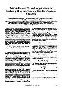
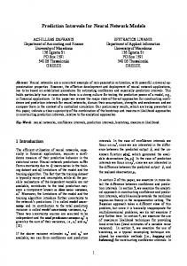
Fig. 2. Predicted vs measured OC for St. Louis four-input network.
much better validation performance than any of the MLR models and was slightly superior to the networks with two, four, and five inputs. For comparison, the best MLR model for this field was the four-regressor model with SSE values of 1.74 and 6.65 for calibration and validation, respectively. The best network performance for the Outlook field included four inputs and achieved SSE values of 0.37 and 0.67 in calibration and validation testing, respectively. The best MLR model utilized the same inputs and had a similar calibration SSE (0.30) but a larger validation SSE value of 1.56. Data points in Fig. 1 were tightly clustered with low OC contents and displayed nearly equal dispersion above and below the ideal unity-slope line. For the Swift Current field samples, the neural networks again performed better in validation than did the MLR models, with the five-input network having the best calibration and validation SSE values, 0.75 and 1.27, respectively. In contrast, the best MLR model used three regressors and had SSE values of 0.87 and 1.95 for calibration and validation, respectively. For the Watrous field data, the neural networks and MLR models displayed similar performance, with the networks performing slightly better. The best network used the same two inputs as the best MLR model. Calibration SSE values were similar for the network and linear model (2.28 and 2.54, respectively), but the network performed better during validation (SSE values were 5.10 and 7.73, respectively, for the network and linear model). The best network identified for the St. Louis field had four inputs, which were the same as those used in the best MLR model. Performance of the neural networks was similar to the performance of the MLR models for this field. The best network was only slightly better than the best MLR model, with calibration and validation SSE values of 3.26 and 4.82, respectively, for the network and 4.03 and 5.93, respectively, for the MLR model. The scatter plot (Fig. 2) showed no tendency for the network to under- or overestimate OC content. Data points were more widely dispersed about the ideal line than with other fields, however. This greater dispersion corresponded to a relatively large validation SSE value, considering that only 30 samples were present, versus 45 for the other four fields. Note that the range of OC contents in the St. Louis field was much greater than for the Outlook field.
For three fields (Outlook, Watrous, and St. Louis), the best neural network used the same inputs as the best MLR model. For the remaining two fields (Hepburn and Swift Current), the network with the best performance used different inputs. However, networks using the best MLR inputs for the latter two fields still provided very good performance. This appeared to confirm the strong correlation between the wavelengths selected and the OC content of the soils. At the start of network training, networks were automatically initialized with random weight and bias values. Thus, slightly different results were achieved even when training networks with identical architectures on the same data. However, the rapid training available with the current software allowed for multiple training sessions to be carried out within minutes. This contrasts with the experience of Sudduth (1991), who stated that one training session of 10 000 epochs required 49 hours, illustrating the improvements in processing speed achieved in the last decade. Overall, the neural networks provided improved predictive performance over the MLR models. The effort required to calibrate the MLR models and neural networks was similar, with MLR model selection and neural network training procedures requiring about the same amount of time and processing resources. A hardware implementation of a neural network would be significantly more complex than for a MLR model however, which should be considered when designing an infield sensor system.
7.4
CONCLUSIONS and RECOMMENDATIONS Twenty-five neural networks were trained for soil OC prediction using reflectance data as inputs. Calibration and validation data sets and input wavelengths were the same as previously used for MLR model development. The best network for each field was selected, and network performance was compared to that of the best MLR models. Neural networks provided superior predictive performance when compared with previously developed MLR models, even though the wavelengths used as network inputs were selected based on optimum linear model performance. Further improvements in predictive accuracy may be possible through selection of inputs to maximize nonlinear model performance.
LE GÉNIE DES BIOSYSTÈMES AU CANADA
INGLEBY and CROWE
Network development was greatly simplified by the availability of built-in network architectures and training routines in the software. Implementation of neural network modeling for predicting soil OC contents using reflectance data in a practical sensor system thus appears very promising. Prior to development of a soil OC sensor for field use, significant research efforts will be required to extend this work from the laboratory to the field. The effects of soil particle size, moisture levels, and surface debris on soil reflectance must be investigated in order to develop robust predictive models. To function across a range of soil types, the effects of soil parent materials on reflectance must be accounted for during calibration. Future work should also seek to identify the optimum input set for nonlinear predictive models. Variable selection routines for MLR models are already incorporated in statistical software. Development of similar algorithms for neural networks and other nonlinear modeling methods should be feasible. Performance of neural networks with optimized inputs is expected to be excellent. Such networks would be suitable for use in a practical real-time soil OC sensor. REFERENCES Brown, R.B. and J.-P.G.A. Steckler. 1995. Prescription maps for spatially variable herbicide application in no-till corn. Transactions of the ASAE 38(6): 1659-1666. Chen, S., K.-W. Hsieh and W.-H. Chang. 1999. Neural network analysis of sugar content in fruit juice. ASAE Paper No. 993083. St. Joseph, MI: ASAE. Demuth, H. and M. Beale. 1998. Neural Network Toolbox For Use With MATLAB, User’s Guide, Version 3. Natick, MA: The MathWorks Inc.
Volume 43
2001
Ingleby, H.R. 1999. Spectral reflectance measurements for organic matter sensing in Saskatchewan soils. Unpublished M.Sc. thesis. Department of Agricultural and Bioresource Engineering, University of Saskatchewan, Saskatoon, SK. Ingleby, H.R. and T.G. Crowe. 1999. Spectral reflectance measurements for organic matter sensing in Saskatchewan soils. Canadian Agricultural Engineering 41(2): 73-79. Ingleby, H.R. and T.G. Crowe. 2000. Reflectance models for predicting organic matter in Saskatchewan soils. Canadian Agricultural Engineering 42(2): 57-63. Jenkinson, D.S. 1988. Soil organic matter and its dynamics. In Russell’s Soil Conditions and Plant Growth, 11th edition, ed. A. Wild, Ch. 18, 564-607. New York, NY: John Wiley & Sons, Inc. Kushwaha, R.L. and Z.X. Zhang. 1997. Artificial neural networks modelling of soil-tool interaction. ASAE Paper No. 97-3067. St. Joseph, MI: ASAE. Liu, J. and C.E. Goering. 1999. Neural network for setting target corn yields. ASAE Paper No. 99-3040. St. Joseph, MI: ASAE. Sudduth, K.A. 1991. Analysis methods for multivariate data. ASAE Paper No. 91-3034. St. Joseph, MI: ASAE. Sudduth, K.A. and J.W. Hummel. 1991. Evaluation of reflectance methods for soil organic matter sensing. Transactions of the ASAE 34(4): 1900-1909. Sudduth, K.A. and J.W. Hummel. 1996. Geographic operating range evaluation of a NIR soil sensor. Transactions of the ASAE 39(5):1599-1604.
CANADIAN BIOSYSTEMS ENGINEERING
7.5