Improved Models for Predicting Ferrite Content in ...

Improved Models for Predicting Ferrite Content in Stainless Steel Welds J. M. Vitek and S. A. David Oak Ridge National Laboratory Oak Ridge, Tennessee 37831-6096 U. S. A.

Abstract As-welded ferrite content in stainless steels has a strong influence on weld properties. In addition, it can be used as an indicator of the solidification mode during welding. In the last 60 years, constitution diagrams have been used to predict ferrite content as a function of weld composition. Over the years these constitution diagrams have been improved but the basic approach used in the diagrams has not changed. Ferrite level is predicted as a function of chromium and nickel equivalent factors, which are determined by taking a weighted sum of specific alloying additions. These diagrams have been found to be very useful, but they are subject to important limitations. More recently, a new approach using artificial neural networks for predicting ferrite content in welds has been proposed. This approach has the advantage that complex interactions among alloying additions can easily be taken into account. This paper describes two such models that have been developed. The first predicts Ferrite Number (FN) as a function of composition only. This model is far more accurate than constitution diagrams in predicting FN over a wide composition range. A second neural network model has been developed more recently. This model quantitatively considers the influence of cooling rate and welding conditions on FN for the first time, an effect that is particularly important for laser welding, high speed welding, and welding of duplex stainless steels. The paper concludes with remarks on future directions for improvement in predictive models.

Introduction Stainless steel welds characteristically consist of two-phase austenite plus ferrite microstructures. Ferrite levels may vary from a few percent in austenitic stainless steel welds to more than 50% in duplex stainless steel welds. The ability to predict the ferrite content in these welds is essential for many reasons. To a large extent, the final ferrite content determines a weldment’s properties such as strength, toughness, corrosion resistance, and long-term phase stability. In addition, ferrite content is a useful

indicator of the mode of solidification, which strongly influences the hot-cracking propensity during welding. Over the years, various models have evolved to try to accurately predict the ferrite content in stainless steel welds*. Constitution diagrams, in which the overall alloy composition is converted into two factors, a chromium equivalent (Creq) and a nickel equivalent (Nieq), have been developed to predict FN in welds. One of the earliest constitution diagrams was that introduced by Schaeffler1. Many modified diagrams have been proposed since then2-7, with the WRC-1992 diagram7 being the most recent and most accurate. The various versions of constitution diagrams differ primarily in the coefficients that are used to convert the alloy composition into the Creq and Ni eq; an extensive review is given in reference 5. In most commonly used constitution diagrams, the weighted coefficients are constant, and this means that a given alloy addition’s influence is the same regardless of that element’s concentration or the concentration of any other alloying additions. In those cases where non-constant coefficients were proposed, the applicability of the diagram is limited to a restricted composition range. Clearly, constant coefficients cannot represent real behavior very well. For example, the effect of carbon should be very different depending on whether carbide forming elements are present or not. This limitation has been removed with the development of predictive models based on artificial neural network analyses8-11. Artificial neural networks are ideally suited for predicting ferrite content because they offer improved flexibility, robustness, and accuracy as a consequence of their use of non-linear regression methods. In this paper, two recently developed neural network models will be described. In the first, the predicted FN is based on the alloy composition, taking into account 13 different alloying additions. This model is significantly more accurate than the most recent constitution diagram. The second neural network

*Strictly speaking, ferrite content refers to a volume % ferrite while FN is an indicator of ferrite level but is not equal to the volume %. In this paper, ferrite content and FN will be used interchangeably to specify ferrite level. Vitek, page 1of 6

model considers cooling rate as well as composition as inputs to the model. It is well documented that cooling rate can have a significant impact on the final ferrite content12-19. Cooling rate can influence the ferrite level in two ways: (a) it can change the mode of solidification from primary ferrite formation at low cooling rates to primary austenite formation at high cooling rates, and (b) it can suppress the solid-state transformation of ferrite to austenite after solidification, with the extent of suppression increasing with increasing cooling rate. The effect of cooling rate was considered qualitatively by David et al14 but the new neural network model accounts for cooling rate effects quantitatively.

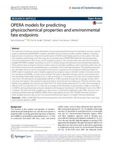
Neural Networks - General Neural networks are sophisticated non-linear regression routines that, when properly “trained”, allow for the identification of complex relationships between a series of inputs and one or more outputs. Networks consist of three layers: input, hidden, and output layers. Each layer contains nodes and the nodes from different layers are connected, as shown schematically in Fig. 1. The nodes correspond to specific inputs and outputs in the first and last layers, respectively. In the case of the FN neural networks, the input layer nodes are elemental concentrations (and cooling rate for the cooling-rate-inclusive network) and the single output layer node is the Ferrite Number. The value at one node is determined by a weighted sum of the nodes in the preceding layer. Training involves a repetitive process in which inputs are used to calculate the outputs, and these outputs are compared with the experimental output. Corrections to the weight factors that connect nodes are made so as to minimize the error between the calculated and actual output. The reader is referred to the literature for further details on neural networks in general20-21, and the FN neural networks in particular8,11.

Data Generation As described above, the development of a neural network involves training of the network with a training dataset that includes inputs (composition and cooling rate) and the associated outputs (FN). The accuracy and applicability of a neural network

Figure 1: Schematic diagram of a neural network showing the three layers and the connections between nodes. The lines connecting nodes are shown with different weights to indicate the variation in weight factors between nodes.

is determined to a large extent by the training dataset that is available - the larger the dataset, and the greater the range of inputs that it covers, the better the final network that is produced. For the composition-only neural network, the same data that were used to produce the WRC-1992 constitution diagram were used to generate the neural network model. This dataset was a compilation of data from several sources8. Thirteen elements were considered in the network: Fe, Cr, Ni, C, N, Mo, Mn, Si, Ti, Cu, V, Nb, and Co. In some cases, the concentrations of all of these elements were not available and how this deficiency was addressed is described in reference 8. For the cooling-rate-inclusive neural network, supplemental data from the literature were added to the WRC-dataset. In addition, new data were generated on a variety of austenitic and duplex stainless steel laser and high-speed arc welds. There were several problems that had to be addressed in generating the dataset for the cooling-rate-inclusive network. These included determining the cooling rate as a function of weld conditions, assigning a cooling rate to the extensive WRC-1992 data, and converting volume % ferrite measurements to FN. These issues and their resolution are described in detail elsewhere11.

Composition-Only Neural Network Model The composition-only neural network that is described here has been documented in detail elsewhere8-9 and has been named FNN-1999. Recently, another composition-only neural network has been developed10, using the same WRC-1992 dataset. Both models are significantly more accurate than the WRC-1992 constitution diagram. In this paper, results from the FNN-1999 model will be considered. A comparison of the WRC-1992 and FNN-1999 models is shown in Figs. 2a and 2b, where the calculated FN are plotted against the measured FN. It is clear that the degree of scatter is significantly reduced with the FNN-1999 model. Quantitatively, the root mean square (RMS) errors for the two models are 5.8 and 3.5, respectively, representing a 40% improvement for the FNN1999 model. The plots in Fig. 2 represent the degree to which the models can fit the data, and therefore they do not indicate the predictive accuracy of the two models. The predictability was assessed by comparing the predicted values with experimental values on another dataset that was not used in the model development9. For this comparison, the FNN-1999 neural network model also showed a significant improvement over the WRC-1992 model, with RMS errors of 2.3 and 2.6, respectively, corresponding to a 12% improvement. Perhaps the most significant advantage of the FNN-1999 model is that it allows for the effect of various elemental additions to change with overall alloy composition. Such variations in the influence of elemental additions were indicated by experimental measurements. For example, the model predicted that the effect of Si in an austenitic stainless steel is to increase the ferrite level at low Si concentrations but to decrease the FN slightly at higher Si contents9. As another example, it was predicted that the effect of V is reversed when considering an austenitic versus a duplex stainless steel. In the former, V decreases the FN slightly while Vitek, page 2of 6

in the latter, V increases FN significantly9. The same ability to identify elemental effects that vary with overall alloy composition was found for the other neural network model as well10. Thus, the neural network models are more accurate than the traditional constitution diagram and furthermore, they allow for greater flexibility when identifying the effects of alloying elements on FN.

Cooling-Rate-Inclusive Neural Network Model

Figure 2: Plots of predicted FN versus measured FN for the WRC1992 dataset. Predictions are made using the three different models: (a) WRC-1992, (b) FNN-1999, and (c) ORFN© .

As noted earlier, it has been well documented that cooling rate can have a strong influence on the as-welded FN. A new neural network model (ORFN©) has been developed recently that takes the cooling rate into account by adding a 14th input node corresponding to cooling rate11. The additional cooling rate variable is calculated using a simple analysis11 and may not be an accurate representation of the actual cooling rate. However, the analysis does not require the accurate calculation of the cooling rate11. Instead the requirement is that it accurately represents relative cooling rates for different weld conditions and this is expected to be the case. The calculated FN versus measured FN using the ORFN© model is shown in Fig. 2c for the WRC dataset. Examination of Figs. 2a, 2b, and 2c shows that the ORFN© model is comparable to the FNN-1999 model and is significantly more accurate than the WRC-1992 model. The RMS error for the ORFN© model is 3.9, or roughly the same as that for the FNN-1999 model. When examining the predictability of the new ORFN© model on an independent dataset, the RMS error for ORFN© is 1.8, or 22% better than FNN-1999 and 21% better than WRC-1992. The real advantage of the new, cooling-rate-inclusive ferrite prediction model is demonstrated when one examines data that include welds made at high speeds or with high power density processes (laser welds), where high cooling rates prevail. The predicted versus measured FN for the larger dataset that included laser weld data and high speed arc weld data is shown in Figs. 3a, 3b, and 3c, for the WRC-1992, FNN-1999, and ORFN© models, respectively. It is readily apparent that the two former models show a large degree of scatter compared to the latter model. Quantitatively, the RMS errors for the three models are 9.9, 11.0, and 4.7, respectively, corresponding to an improvement for the ORFN© model of over 50%! In Figs. 3a and 3b, a series of points are encircled. These data represent one example where FN measurements were made on welds of the same alloy but welded at different speeds and powers, and therefore different cooling rates. The WRC-1992 and FNN-1999 models predict the same FN value for all weld conditions since they do not take cooling rate into account. Thus, the agreement between experimental measurement and prediction is poor. This limitation is removed in the ORFN © model, resulting in a significant improvement in the accuracy of the predictions. A few examples of predictions using the ORFN© model will now be considered. In Fig. 4, the calculated FN is plotted as a function of the cooling rate (log scale) for a typical 308 stainless steel alloy composition. The predictions show a gradual increase in FN with cooling rate that is a consequence of the increasing degree to which the ferrite-to-austenite solid state transformation Vitek, page 3of 6

a)a)

Figure 4: Plot of predicted FN versus log cooling rate for a type 308 austenitic stainless steel (Fe-20.15Cr-10.68Ni-0.059C0.026N-1.92Mn-0.78Si-0.38Ti) using the ORFN© model.

b)b)

c)

c)

Figure 3: Plots of predicted FN versus measured FN for the expanded dataset that includes high-speed welds, laser welds, and additional duplex stainless steel welds. The predictions are made using the three different models: (a) WRC-1992, (b) FNN-1999, and (c) ORFN© .

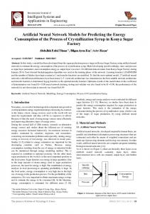
is suppressed as cooling rate increases. An increase in FN from ~15 to ~27 is predicted. Beyond a calculated cooling rate of ~104 °C/s, the FN decreases and this reflects the fact that the solidification mode changes from primary ferrite to primary austenite formation. Eventually, at calculated cooling rates greater than ~3x106 °C/s, the predicted FN is 0, indicating complete austenite solidification with no ferrite formation. The predicted variation of FN with cooling rate agrees with what is expected based on an understanding of the solidification and solid-state transformation behavior. The trend also agreed with experimental data11. It should be kept in mind that these results apply to the particular composition used for the alloy and they will vary as the alloy composition changes. A second example is shown in Fig. 5, where the predicted FN is plotted against peak power for a pulsed laser weld at constant weld speed. The alloy composition is the same 308 austenitic stainless steel composition that was used in Fig. 4. In this example, decreasing weld power corresponds to an increasing cooling rate. Once again, FN is predicted to increase with increasing cooling rate (decreasing laser power) to a maximum of ~27 and then FN is predicted to decrease, eventually reaching 0. In Fig. 5, the FN at the maximum power considered is ~21, which is larger than the FN at low cooling rates in Fig. 4, indicating that even at this high laser power, a moderately high cooling rate is expected and a higher FN than that found at low cooling rates is predicted. A final example is shown in Fig. 6, where the predicted FN is plotted versus sample thickness for a GTA weld on a type 312 stainless steel alloy. For duplex steels, the FN will increase monotonically with increasing cooling rate as the solid state transformation of ferrite to austenite is increasingly suppressed. For these alloys, the switch in solidification mode at high cooling rates, as found in austenitic stainless steels, will not take place. The model predicts that the as-welded FN will increases gradually from ~90 to ~110, corresponding to a nearly fully ferritic microstructure. The slight “hump” in the predicted FN versus thickness is an artefact due to the transition from 3D to 2D cooling conditions. In general, the ORFN© model predicts that the FN of duplex Vitek, page 4of 6

Figure 5 Plot of predicted FN versus pulsed laser power for a type 308 austenitic stainless steel (Fe-20.15Cr-10.68Ni-0.059C0.026N-1.92Mn-0.78Si-0.38Ti) using the ORFN© model.

Figure 6: Plot of predicted FN versus sample thickness for a type 312 stainless steel (Fe-29.92Cr-8.78Ni-0.11C-0.01N-1.68Mn0.2Mo-0.39Si) using the ORFN© model.

stainless steels will be sensitive to cooling rates at moderate values while the FN of austenitic stainless steels will vary the most at high cooling rates. A more detailed evaluation of the ORFN© model is presented in reference 11. There, the predictions are compared with experimental data and good agreement is found. The initial increase followed by a subsequent decrease in FN for austenitic stainless steels agrees with measured results. For duplex stainless steels, the gradual increase in FN also agrees with experiment. The model predictions are in stark contrast to those of the WRC-1992 and FNN-1999 models (and in fact all previous FN prediction models) which predict the same FN for a given alloy regardless of the weld conditions.

calculating the cooling rate based on the weld condition inputs and then using the calculated cooling rate as an input for the neural network model calculation. One characteristic of neural network models is that a unique model does not exist. Therefore, it is likely that future model developments will result in improved prediction capabilities, especially if additional, reliable data are used to train the networks. There are several assumptions and simplifications that were used in the development of the cooling-rate-inclusive model that should be mentioned. First, cooling rates were calculated using the simple Rosenthal equations11,22. A methodology for transitioning from 2D to 3D cooling conditions was developed and this was satisfactory but not perfect*. It must be noted that the model development requires the calculation of the proper relative cooling rates, and it does not require absolute accuracy in the calculation of the cooling rates. Nonetheless, improvements in the cooling rate assessment may be possible. Second, for the WRC portion of the entire dataset, which constituted a major fraction of the total training dataset, weld conditions were not available and cooling rates were assigned to the data. The development of a training dataset where all the cooling rates are calculated based on actual welding conditions would be preferred, but such a dataset is not available. Third, complications arose with respect to the measurement of ferrite content in high speed welds since the welds were small and not amenable to direct FN measurement. Thus, volume % ferrite was determined and a conversion from measured volume fraction ferrite to FN was required for some data. All of these limitations are discussed in greater detail in reference 11. Finally, the FN will vary with position in the weld since the solidification conditions are not uniform across the entire weld. Thus, in principle, it would be useful to add yet another variable in the neural network model development to account for the position within the weld. Such a model could be

Discussion The development of neural network models for predicting FN in stainless steel welds represents a significant improvement over conventional constitution diagrams. Alloying element interactions can be taken into account in a more complete manner, and the influence of additional variables, such as cooling rate, can be readily considered. The implementation of neural networks as a predictive tool has some advantages as well as disadvantages. The primary disadvantage is that, unlike the constitution diagrams, the model cannot be displayed in the form of a convenient figure that could be used directly. Instead, a calculation must be made, based on the values of the input variables and the neural network parameters. However, the calculation is a simple one that can be carried out instantaneously on any computer. The ability to calculate directly the FN can be an advantage to the user. For example, if the neural network is implemented in the form of a spreadsheet, then compositions can be inputted and the variations can be readily found. Parametric studies (as were done in Figs. 4-6) are particularly simple. In addition, the calculations can be programmed for a large dataset and a large throughput is possible. For the ORFN© model, where cooling rate was also considered, the spreadsheet can be set up to use composition and the weld conditions (power, speed, thickness) as inputs. The spreadsheet can then seamlessly predict FN by first

*The “hump” in Fig. 6 is an artefact that is a direct result of the imperfect transition from 2D to 3D cooling conditions as thickness increases. Vitek, page 5of 6

developed but the availability of the appropriate data is a necessity and the creation of such a database would involve a substantially larger effort. In spite of the limitations noted above, the new ORFN© model provides a predictive capability that has been heretofore completely absent. Thus, for example, even though the variation in FN with location within the weld is not known, the model allows one to determine the sensitivity of the FN value to the weld conditions for a given composition. Consequently, reasonable estimates of how the FN will change with location within the weld can be made. The effect of compositional modifications can be readily determined, and thus the relative sensitivity of different alloy compositions can be identified. The ORFN© model was developed for arc and pulsed laser welds and is not strictly applicable to other processes such as EB welding. However, once again, the sensitivity of FN for a given composition to changes in cooling rate can be easily calculated, and realistic estimates of the change in FN with weld conditions for other processes can be made. Thus, a new dimension to alloy design and weld optimization is available with the ORFN© that has been totally absent with earlier FN models.

References 1. 2. 3. 4. 5. 6. 7. 8. 9. 10.

11. 12.

Summary and Conclusions

13.

In the last few years, neural network models for predicting FN in stainless steel welds have been developed. These models are significantly more accurate than previously-developed constitution diagrams. Two neural network models were described in this paper. The first is a composition-only model that uses the concentrations of 13 elements to predict FN. The second model has been developed more recently and it includes cooling rate as well as composition when predicting FN. This latter model, ORFN©, represents the first prediction model that quantitatively accounts for the effect of weld conditions on FN. The ORFN© model correctly predicts the variation in FN due to solidification mode changes and suppression of the solid-state ferrite to austenite transformation at high cooling rates. The ORFN© model is particularly useful for high-speed welds, duplex stainless steel welds, and high-power density process welds, but it is applicable to all conditions.

14. 15. 16. 17. 18.

19. 20. 21. 22.

A. Schaeffler, Metal Progress, 56, 680-680B (1949) F.C. Hull, Weld. J., 52, 193s-203s (1973) W.T. DeLong, Weld. J., 53, 273s-286s (1974) N.I. Kakhovskii, V.N. Lipodaev, and G.V. Fadeeva, Avt. Svarka, 5, 55-57, (1985) D.L. Olson, Weld. J., 64, 281s-295s (1985) T.A. Siewert, C.N. McCowan, and D.L. Olson, Weld. J., 67, 289s-298s (1988) D.J. Kotecki and T.A. Siewert, Weld. J., 71, 171s-178s (1992) J.M. Vitek, Y.S. Iskander, and E.M. Oblow, Weld. J., 79, 33s-40s (2000) J.M. Vitek, Y.S. Iskander, and E.M. Oblow, Weld. J., 79, 41s-50s (2000) M. Vasudevan, M. Murugananth, and A.K. Bhaduri, to be published in Mathematical Modeling of Weld Phenomena, Institute of Materials, London (2002) J.M. Vitek, S.A. David, and C.R. Hinman, submitted for publication in Weld. J. (2002) J.M. Vitek, A. DasGupta, and S.A. David, Metall Trans A, 14A, 1833-1841 (1983) S. Katayama, and A. Matsunawa, ICALEO 84, Laser Inst America, Orlando, FL, 44, 60-67 (1984) S.A. David, J.M. Vitek, and T.L. Hebble, Weld. J., 66, 289s300s, (1987) M. Bobadilla, J. Lacaze, and G. Lesoult, J. Cryst. Growth, 89, 531-544 (1988) J.W. Elmer, S.M. Allen, and T.W. Eagar, Metall Trans A, 20A, 2117-2131 (1989) J.C. Lippold, Weld. J., 73, 129s-139s (1994) J.M. Vitek and S.A. David, Laser Materials Processing IV, eds. J. Mazumder, K. Mukerjee and B. L. Mordike, TMS, Warrendale, PA, 153-167 (1994) T. Koseki and M.C. Flemings, Metall Mater. Trans A, 28A, 2385-2395 (1997) D.E. Rumelhart, B. Widrow, and M.A. Lehr, Comm. ACM, 37, 87-92 (1994) C.M. Bishop, Rev. Sci. Instr., 65, 1803-1832 (1994) D. Rosenthal, Weld. J., 20, 220s-234s (1941)

Acknowledgments This research was sponsored by the U. S. Department of Energy, Division of Materials Science and Engineering and the U. S. Department of Energy Laboratory Technology Research Program, under contract DE-AC05-00OR22725 with UT-Battelle, LLC.

Vitek, page 6of 6