Neural Network Prediction of Radio Propagation - Semantic Scholar

AUSTRALIAN COMMUNICATION THEORY WORKSHOP PROCEEDINGS 2005

1

Neural Network Prediction of Radio Propagation Lei Qiu, Danchi Jiang and Leif Hanlen

Abstract— Preliminary work for predicting signal distributions in a local area, using a feature-based neural network is presented. The neural network is trained by radio signal measurements at known positions. After appropriately setting the parameters of nodes of the neural network, a corresponding virtual propagation environment is built, which reasonably represents the actual environment. Radio signal strength distribution is predicted by the virtual environment. A new method for radio signal measurement is introduced which mitigates the effect of small scale fading when determining the fingerprint of a position. Index Terms— radio propagation, neural networks, radio measurement, IEEE 802.11b

I. I NTRODUCTION Prediction of radio propagation in indoor environments is known to be a difficult problem, due to reflection, diffraction and scattering of radio waves. Numerous statistical and deterministic radio propagation models are available for predicting wireless signal spatial and temporal distributions [1–4]. The performance of these models is unsatisfactory due to their accuracy and/or computational complexity, especially in propagation environments with dense multi-path such as indoor scenarios. Many predictive methods use ray-tracing as a foundation [5]. Ray-tracing is a well known, and widely used radio propagation model, based upon the approximation of wireless signals as linear rays emanating from a point-like source. The rays are straight lines, perpendicular to the wavefront, possibly augmented with reflections and/or scattering [5, 6]. The model has been used in several scenarios, for example [1, 7] and takes its intuition from physical optics. Although raytracing is an effective theoretical tool for indoor wireless environments [8], a fine spatial resolution is required for accurate prediction. The cost of computation increases with increasing sample resolution and the details of structures along radio propagation path are critical to final prediction results. At high resolution, ray-tracing typically incorporates so-called “small scale” fading which varies on the order of a few wavelengths. However, for point-like receivers small scale fading is essentially not predictable for ranges beyond halfwavelength [11]. Moreover, including small-scale fading does not provide useful predictive information. For these reasons, we develop a ray-tracing like model which attempts to accurately match large-scale fading effects in the channel. We define large-scale fading as variations L. Qiu is with National ICT Australia, and the Australian National University, Canberra L. Hanlen and D. Jiang are with National ICT Australia, Locked Bag 8001, Canberra ACT 2601 Australia, and affiliated with The Australian National University, Canberra ACT 0200, Australia. National ICT Australia is funded through the Australian Government’s Backing Australia’s Ability initiative, in part through the Australian Research Council. e-mail: {Lei.Qiu,Danchi.Jiang,Leif.Hanlen}@nicta.com.au.

which are temporally and spatially coherent over a nonnegligible range. Specfically, for a “position” in space-time {r, t}, we expect that the fading at a “nearby” position {r + δ, t} will have similar characteristics, for δ  λ. We apply a feature-based neural network learning algorithm to predict the received radio signal distribution as a function of position r based on off-line measurements. We produce a “virtual environment model” where dominant features such as reflective walls and scattering bodies are provided as model parameters. We set up a neural network to “learn” this environment based on the wireless signal strength measured at particular (stochastic) positions. We use the trained neural network to predict the radio signal strength. Experimental results demonstrate the effectiveness of this algorithm. The remainder of this paper is arranged as follows. In section II two radio propagation models are given as preliminaries. We outline the characteristics and efficacy of the models. In section III provides an introduction to feature-based neural networks. The neural network learning algorithm is discussed in section IV. Section V shows how to set up the experiment and measurement examples. The “stochastic method” is compared with common static measurement approaches. The measured radio signal distribution and the learned signal distribution are compared in section VI and the prediction performance based on the two propagation models is analyzed. The last section is devoted to the conclusion and discussion of future work. II. R ADIO P ROPAGATION M ODELS Consider a frequency-flat fading environment, where the channel is given by y = ax + n and y is the receive symbol, x is the transmit symbol with (complex scalar) channel gain a and AWGN sample n. The channel comprises L paths, and the signal received is a weighted sum of signals from each path without ISI. This is the well-known discrete model for multipath channels [9, 10], such that L X a= |αi | e−jφi i=1

For any channel model, we must trade off prediction reliability with computation expense, and measurement resolution. In our case, we are limited to signal strength (real power) measurements. We consider two simple models for the power received at a particular point r in space. • Model 1: the signal received is a phasor sum of complex signals, which result in a particular real power. In this way, the common phasor model for electric signals provides a hidden model for the received power.

2

AUSTRALIAN COMMUNICATION THEORY WORKSHOP PROCEEDINGS 2005

•

Model 2: all received power is assumed to be a weighted sum of coherent power blocks (no phasor component) – so the underlying electrical source of the power measurement is ignored. The name “coherent power” reminds the reader that the underlying signals are effectively all in phase.

A. Propagation Model 1: electric signal Consider a single path, of a multi-path environment. An electric signal arrives at the receiver with phase (and amplitude) determined by path length and reflection characteristics. The electric field with distance di to transmitter at time t is given by [5]   2πdi E0 d 0 cos x(t) (1) Ei (di , t) = Γi di λ where E0 is the electric field (V/m) at a reference point with distance d0 to transmitter, λ is the wavelength of the radio wave. The constant Γi is the reflected field strength, in the case that the wave is reflected. For multiple waves the total electric field at a position is the scalar sum of all the components (LOS and/or NLOS) given by X E(r) = Ei (r) (2) i

The corresponding received signal power at the position r is [5] |E(r)|2 Gr λ2 Watts (3) P (r) = 480π 2 This model includes small scale fading, as is typically used for scattering models. Note that the power P is the “model parameter” which will be measured, not E. B. Propagation Model 2: coherent power Prediction of small-scale fading statistics is known to be an ill-posed problem [11]. Given the power measurements available at the receiver, we wish to estimate the value of a “large-scale” fading process: ie, one which may be modelled without recourse to phase information. For a multi-path signal, each path contributes to the power at receive location r. The power contributed by the k th path is [8] αP0 Y Pk (r) = σi (4) lk (r)2 i where Pk (r) is given directly from signal-strength measurements. Here α is a constant, related to the antenna pattern, carrier frequency and initial path direction, P0 is the transmitter power, lk (r) is the length of the unfolded path from transmitter to location r via path k, σi is the transmission or reflection coefficient of the ith wall along the path. We assume only a single reflection per path in this paper, so the total power at a position is given by P (r) =

L X k

L X αP0 σk Pk (r) = lk (r)2

may be arranged to perform equally well with the full phasor sum of model 1, under the relaxation that σ may take on negative values. III. N EURAL N ETWORKS AND L EARNING A LGORITHMS Artificial neural networks are well-developed for learning functional relationships [12] and comprehensive reviews exist, such as [13]. Artificial neural networks arise from imitations of biological neural systems, providing a simple application of parallel computation and have been extended to solve system learning and optimization problems [14, 15]. Any function may be approximated by a piece-wise linear function, which we shall denote as a “basis function”. Let φ(k, ρ) be the general basis function used for approximation, where k is the index of the function and ρ is the state. We may consider the state in terms of function samples, where the function is evaluated at a finite set of “states” ρi , i = 1, 2, . . .. Where there is no ambiguity, we shall interchange the state ρi and in index i. A function J(ρ) can be approximated by a basis: K X ˜ r) = J(i, rk φk (i), (6) k=0

where r = {r1 , . . . rK } are the weights associated with the basis set {φ0 (i), ..., φK (i)}. The best approximation, in an MMSE sense, for a given set of basis functions may be obtained via solving: 2 X ˜ r) . r = arg min (7) J(i) − J(i, r∈RK+1

i

Equation (6) represents a single layer neural network. For more complex (or higher dimensional) functions, multiple layers may be used. Such multi-layer neural networks are said to contain “hidden layers” which are composites of two or more single layer networks such as: ! K L X X ˜ r) = J(i, r(k)σ r(k, l)xl (i) , (8) k=1

l=1

where the base function σ(s) is a smooth monotonic function taking values in (0, 1) or such a function taking values in (−1, 1). i.e., 1+e1 −s or tanh(s). Sometimes, there are functions of the state known to be important or useful in the prediction. In these cases, intermediate functions, called features, are introduced to capture the important aspects of the current state. Let the feature vector associated with state i be denoted as f (i),Pthe single layer ˜ r) = network now can be written as J(i, k r(k)φk (f (i)). Features can be obtained by prior-knowledge of the network or heuristic policies. In this paper, the radio propagation models are used as feature functions. IV. F EATURE -BASED N ETWORK D ESIGN

(5)

k=1

Model 2 assumes no phasor effects in the field received: all signals arrive at the receiver coherently. We conjecture model 2

Both generic and kernel-based neural networks have been applied to the study of signal strength measurement and prediction issues, see for example [16, 17]. However, previous work has focussed on the application of generic learning

NEURAL NETWORK PREDICTION OF RADIO PROPAGATION

3

methods to the special class of the signal strength of wireless communication. In this paper, we use the feature-based learning method, which incorporates the special feature of the signal strength model under consideration. Rather than choose the usual sigmoidal function, as the basis, we use either radio propagation model 1 or model 2 instead. As such, the neural network itself has a strong physical meaning. In addition, because the neural network basis is selected closely with the real model, it is expected the resulted method can be more efficient and effective. At the off-line stage we measure the received signal at given positions and use this data to train the feature weights of the neural network, which are in the the hidden layer. The features are the position and reflection coefficient of reflectors (walls) or scatters. The output layer is the Neural Network cost function J, the difference between the measured power distribution and the estimated power distribution. The parameters of walls are adjusted according to the given power distribution map of a certain area, which has a certain grid size. In the one dimensional case, P (m) is the power at position rm where m = 1, 2, . . . , M . There are M known positions stored in database, and each rm is a labeling of a physical location. Since m uniquely specifies rm we may consider P as a function of m. We assume we know the position and reflection coefficient of N ideal walls, either from an iteration or an initial guess. Each wall will reflect its incident wave and contribute a signal component to a certain position rm . We either use propagation model 1 or model 2 to calculate the estimated power distribution P¯ (m, R) at the position rm . Here R is the array of the parameters of the N walls. The cost function J is defined as J=

M 2 1 X P (m) − P¯ (m, R) 2 m=1

(9)

and minimized by the fixed point equation: Rk+1 = Rk − γ

∂J ∂Rk

(10)

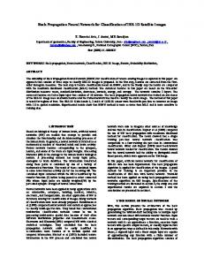
We set a threshold  for the cost function J, and for J <  the fixed point iterations are terminated. V. E XPERIMENTAL M EASUREMENT S ETUP For field measurements the Compaq N800V installed with Lucent ORiNOCO Gold 802.11b WLAN adaptor [18] was used as a measurement device. A single Lucent ORiNOCO AP-1000 Access Point (AP) was deployed as the transmitter. The Operating System (OS) for the laptop was Redhat 9.0 with kernel updated to 2.4.27. The adaptor driver version is 0.13-d [19] patched the scanning patch by Pavel Roskin [20, 21], Wireless Extension and Wireless tools [22] provide the received signal strength from different APs. The laptop uses Wireless Tools v.26 and Wireless Extensions v.16. The field measurements were taken at the National ICT Australia office in Canberra, Australia, shown in Figure 1. The transmitter was located at the end of a corridor and measurements were taken along the length of the corridor.

Fig. 1. NICTA Building, at Northborne Ave, Canberra. Line of measurements along corridor shown at left-hand edge. North is at top of page.

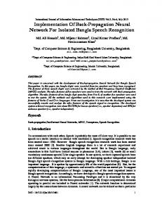
A. Static Method The receiver was placed at a position and the distance between receiver and transmitter measured. Then we ran a TCL/TK script to scan all the available APs in the neighborhood and store their signal strengths in database. After one second, we repeated the scanning again until the Maximum Scanning Number (MSN) is reached. The mean and maximum values of the MSN signal strengths at each position was stored. During the measurement cycle, the receiver position was held fixed. In the static measurement experiment small scale fading is observed. In Figure 2 we take M SN = 20 samples at a position. T /R distance means the distance between the transmitter and receiver. The unit of received signal power at the receiver is dBm. The measurement step size within distance from 380cm to 550cm is 5cm. Experiment results show the signal strength is stable in the temporal scale while suffering severe (and unpredictable) fading in the spatial scale. This is because small scale fading is typically due to phase effects and occurs on spatial scales smaller than a wavelength (λ ≈ 12cm). In dense multi-path, prediction of the fading characteristics is ineffective for extrapolation beyond approximately one wavelength λ [11], under the experimental setup used. Similar observations have been made in the temporal case [23] B. Fuzzy sampling method Given only simple power measurements, a metric is desirable which estimates the large scale fading characteristics of the field, without inappropriate emphasis on the small scale, local effects. A natural (statistical) approach would be to take a number of samples within a nearby region and to perform an averaging over the samples. We may ask “Why ignore small scale fading?” the answer to this comes from well known

4

AUSTRALIAN COMMUNICATION THEORY WORKSHOP PROCEEDINGS 2005

−45

−30

Measured Power Final Estimated Power Initial Estimated Power

−50 −55 Power (dBm)

Power (dBm)

−35

−40

−45

−60 −65 −70 −75 −80

−50

−85

−55 300

−90

400

500 600 T/R Distance (cm)

700

Fig. 2. Small scale fading, from measured data along corridor. Note scale is in cm. λ ≈ 12cm TABLE I M ODEL COMBINATIONS

Reflective walls Scattering bodies

Small scale model 1 (static) Ia Ib

Large scale model 2 (fuzzy) IIa IIb

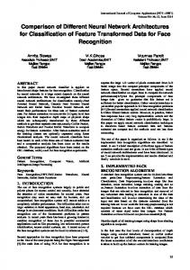
results in extrapolation of functions, such as the Nyquist sampling result, and [11]: if we wish to predict small scale fading, we must sample at well above the maximum rate of change in the fade, which requires known callibration points at a sampling density greater than λ/2. However, large scale fading is dominated by the free-space distance loss in power, and thus has a much lower rate of change over a local area, by comparison, |E(r)| is (approximately) wavelength invariant, and varies at a rate of −2d−3 . For each callibration position r, we measure the received signal strength at a set of positions in the near neighborhood by simply moving the receiver within a nearby region during the MSN scanning process. We use the area-averaged signal strength as the fingerprint of the position. This method is called “stochastic” method. Here the position is not a point but a small area. VI. E XPERIMENT R ESULTS AND A NALYSIS Our objective in this section is to evaluate several model combinations, toward providing a robust and sufficiently accurate modelling procedure. We have four combinations, which we summarise in Table I. In each case the neural network was trained with measurement data at a collection of data points, and the resulting prediction compared with additional points. A. Model 1 results Firstly we use reflectors as the neural network nodes in the hidden layer. The statically measured signal is shown in Figure 3. The transmitter is deployed at the origin. The measurements are performed at distances of 1m, 1.5m, 2m, . . . , 16m

2

4

6

8 10 T/R Distance (m)

12

14

16

Fig. 3. 8 Reflectors with Propagation Model 1. Crosses denote measurements, circled crosses mark training points.

from the transmitter, among which the step size is 0.5m. We use the first radio propagation model with eight reflectors. The circles are the training signal strength at known positions, namely at positions with distances of 1m, 2m, . . . , 16m from the transmitter. The position of the ith reflector is represented by ai X + bi Y +ci = 0. Including the reflection coefficient σi , the weight vector of the ith reflector is defined as [ai bi ci σi ]. All weight vectors constitute the weight matrix for the neural network. With knowledge of position of the reflector, we can calculate the unfolded length from the transmitter to the receiver, based on image theory. Here we only consider simple one-bounce scenario. In the training process, the converging is rather slow when the cost function is approximately equal to 650. The cost function is bounded above 640 as shown in Figure 7. It is shown in Figure 3 that the final estimated power distribution doesn’t match the measured power well. It differs little with the initial estimated power distribution. Given the same measured signal power distribution, we use sixteen scatterers as the hidden nodes. For each node the weight vector is [ai bi σi ], where (ai , bi ) is the X-Y axis of the scatter and σi is the reflection coefficient of the scatter. With phase term included in propagation model, this neural network is efficient in decreasing cost function, which demonstrates the first propagation model has strong capability in fitting the training data. In order to prevent overfitting, the cost function in Figure 4 is 18, though this neural network can converge its cost function close to zero. This figure shows that while the phasor addition model can be easily matched to the trained data, it suffers from wild fluctuations away from the measured data when used to predict signal strength. The reason is simple: small scale fading is highly reliant on local channel parameters, and thus sampling must be performed at or above the Nyquist sampling rate. Sadly, the sampling rate is bounded from above by λ/2 which requires a sampling density of greater than 3 samples per wavelength.

NEURAL NETWORK PREDICTION OF RADIO PROPAGATION

−45

5

0

Measured Power Final Estimated Power Initial Estimated Power

−50

−10

−55 −60

Power (dBm)

Power (dBm)

Measured Power Final Estimated Power Initial Estimated Power

−65 −70 −75 −80

−20

−30

−40

−85 −90

2

4

6

8 10 T/R Distance (m)

12

14

−50

16

Fig. 4. 16 Scatterers with Propagation Model 1. Crosses denote measurements, circled crosses mark training points. Note dominance of small-scale fading.

2

4

6

8 10 12 T/R Distance (m)

B. Model 2 results The prediction accuracy with the second radio propagation model can be improved by using a “stochastic” measurement method. We apply the radio propagation model 2 in our algorithm to train the neural network until the cost function J is relatively small. Once the training process is finished, we apply the weight matrix to calculate signal strength distribution at unknown positions. In Figure 5 four ideal reflectors are acting as the neural network hidden nodes with a final value of cost function around 17. Training signal strength is measured at positions with distances of 1m, 2m, . . . , 17m to the transmitter. The signal fluctuates smoothly, comparing with Figure 4 and Figure 3. We estimate signal distribution at positions of 1.5m, 2.5m, . . . , 15.5m. The error between predicted values and measured values is reasonably small. With the same training signal strength distribution, we used eight scatters as the hidden layer in Figure 6 giving eight nodes. In this figure the final value of cost function is around 14. The prediction can achieve the same level of accuracy as that by reflectors. In Figure 7 the computation complexity for the above four neural networks are given. Entry “Ia” in Table I suffers from the convergence bound of the cost function. “IIa” has similar problems but its bound is much smaller. “Ib” has good performance in converging to the training data but it is poor in signal prediction. “IIb” demonstrates its ability in predicting signal distribution with reasonable computation cost.

16

Fig. 5. 4 Reflectors with Propagation Model 2. Crosses denote measurements, circled crosses mark training points.

−10

Measured Power Final Estimated Power Initial Estimated Power

−20

Power (dBm)

Based on the learned features of the wireless propagation environment, it is possible to predict signal strength at other positions. We use measured signal strength distribution at 0.5m, 1.5m, . . . , 15.5m to validate the predicted values. The prediction result matches the measured data well within a distance of 4 meters from transmitter as shown in Figure 4.

14

−30 −40 −50 −60 −70

2

4

6

8 10 12 T/R Distance (m)

14

16

Fig. 6. 8 Scatterers with Propagation Model 2. Crosses denote measurements, circled crosses mark training points.

VII. S UMMARY AND F UTURE W ORK A new algorithm to predict wireless signal propagation environment, using feature-based neural network was presented. The neural network constructed a virtual propagation environment which reasonably represented the real environment. We apply a new method – “stochastic position” method – in field signal strength measurement. This method mitigates the effect of small scale fading when examining signal strength values. ACKNOWLEDGEMENTS The authors would like to thank Mr. Fergus McKenzieKay and Mr. Kim Holburn for their support in setting up the experiment system. R EFERENCES [1] Z. Chen, H. L. Bertoni, and A. Delis, “Progressive and approximate techniques in ray-tracing-based radio wave propagation prediction mod-

6

AUSTRALIAN COMMUNICATION THEORY WORKSHOP PROCEEDINGS 2005

900

16 Scatterers, Model 1 8 Reflectors, Model 1 4 Reflectors, Model 2 8 Scatterers, Model 2

800

Cost Function

700 600 500 400 300 200 100 0

5

10 15 20 Iteration Number (x 100)

25

30

Fig. 7. Mean square error compared with iteration number. Convergence occurs for cost function equal to zero. Model 1 does not converge as well as model 2, due to large variation. For reflectors (walls) model 1 did not always converge – note large final error for 8 reflectors, model 1.

[2]

[3] [4]

[5]

[6]

els,” IEEE Transactions on Antennas and Propagation, vol. 52, no. 1, pp. 240–251, Jan. 2004. S. Y. Seidel, T. S. Rappaport, S. Jain, M. L. Lord, and R. Singh, “Path loss, scattering, and multipath delay statistics in four european cities for digital cellular and microcellular radiotelephone,” IEEE Trans. Veh. Technol., vol. 40, pp. 721–730, 1991. G. L. T. et. al, “A statistical model of urban multipath propagation,” IEEE Trans. Veh. Technol., vol. 21, pp. 1–9, Feb. 1972. F. Ikegami, T.Takeuchi, and S. Yoshida, “Theoretical prediction of mean field strength for urban mobile radio,” IEEE Trans. Antennas Propagat., vol. 39, pp. 299–302, Mar. 1991. T. S. Rappaport, Wireless Communications, Principles and Practice, 2nd ed., ser. Prentice Hall Communications and Emerging Technologies Series. New Jersey, USA: Prentice Hall, Inc., 2002. R. A. Serway, Physics for Scientists and Engineers, with Modern Physics, 3rd ed., ser. Saunders Golden Sunburst Series. New York, USA: Saunders College Publishing, 1992.

[7] S. Coco, A. Laudani, and L. Mazzurco, “A novel 2-D ray tracing procedure for the localization of EM field sources in urban environment,” IEEE Transactions on Magnetics, vol. 40, no. 2, pp. 1132–1135, Mar. 2004. [8] S. J. Fortune, D. H. Gay, B. W. Kernighan, O. Landron, R. A. Valenzuela, and M. H. Wright, “WiSE design of indoor wireless systems: Practical computation and optimization,” IEEE Comput. Sci. Eng., vol. 2, pp. 58– 68, Mar. 1995. [9] J. G. Proakis, Digital Communications, 2nd ed., ser. Computer Science Series. New York, USA: McGraw-Hill, 1989. [10] B. Sklar, “Rayleigh fading channels in mobile digital communication systems part I: Characterization,” IEEE Commun. Mag., pp. 93–103, July 1997. [11] P. D. Teal and R. A. Kennedy, “Bounds on extrapolation of field knowledge for long-range prediction of mobile signals,” IEEE Trans. Wireless Commun., vol. 3, no. 2, pp. 672–676, Mar. 2004. [12] S. Haykin, Neural Networks: A Comprehensive Foundation. Upper Saddle River, NJ: Prentice-Hall, 1999. [13] Tech. Rep., http://www.dsi.unifi.it/neural/w3-sites.html. [14] D. Jiang and J. Wang, “A recurrent neural network for on-line design of robust optimal filters,” IEEE Transactions on Circuits and Systems - Part I: Fundamental Theory and Applications, vol. 47, no. 6, pp. 921–926, 2000. [15] ——, “On-line learning of dynamic systems in the presence of model mismatch and disturbance,” IEEE Transactions on Neural Networks, vol. 11, no. 6, pp. 1272–1283, 2000. [16] R. Battiti, T. L. Nhat, and A. Villani, “Location-aware computing: a neural network model for determining location in wireless LANs”, Tech. Rep. DIT-02-0083. [17] X. Nguyeny, M. I. Jordanyz, and B. Sinopoli, “A kernel-based learning

[18] [19] [20] [21] [22] [23]

approach to ad hoc sensor network localization”, Tech. Rep. UCBCSD04-1319. OriNOCO, “11bpcard,” Tech. Rep., http://www.proxim.com/products/ wifi/client/11bpccard/index.html. D. Gibson, “Orinoco driver,” Tech. Rep., http://ozlabs.org/people/ dgibson/dldwd/. J. Tourrilhes, “Orinoco information,” Tech. Rep., http://www.hpl.hp. com/personal/Jean“˙Tourrilhes/Linux/Orinoco.html. P. Roskin, “Scanning patch for v.13-d,” Tech. Rep., http://www.hpl.hp. com/personal/Jean“˙Tourrilhes/Linux/Orinoco.html. J. Tourrilhes, “Wireless tools for linux,” Tech. Rep., http://www.hpl.hp. com/personal/Jean“˙Tourrilhes/Linux/Tools.html. Z. Shen, J. Andrews, and B. Evans, “Short range wireless channel prediction using local information,” in The Thirty-Seventh Asilomar Conference on Signals, Systems and Computers, vol. 1, 9–12 Nov. 2003, pp. 1147–1151.