neural networks applied in electromagnetic interference problems

NEURAL NETWORKS APPLIED IN ELECTROMAGNETIC INTERFERENCE PROBLEMS DAN D. MICU1, LEVENTE CZUMBIL1, GIORGIOS CHRISTOFORIDIS2, EMIL SIMION1

Key words: Electromagnetic interference, High voltage power lines, Artificial intelligence, Neural networks, Underground metallic pipelines. Problems regarding the electromagnetic interferences between high voltage power lines and underground metallic pipelines are studied. To evaluate the magnetic vector potential for different constructive geometries of a specific interference problem, a neural networks based artificial intelligence technique is implemented. To find the optimal solution, different neural network architectures are tested. Results gained with neural networks are compared to finite element solutions considered as standard ones.

1. INTRODUCTION In many cases to reduce construction costs and due to government regulations, which restrict access to new right-of-ways, supply utilities (gas, water or oil) are forced to share for long distances the same distribution corridors with high voltage power transmission lines (HVPL) or a.c. railway systems. Taking into account this right of way the gas, water or oil supply underground metallic pipelines (MP) are exposed to induced a.c. currents and voltages. In case of one or two phase faults on HVPL, the induced a.c.voltage in unmitigated MP can reach thousands of volts. This could be very dangerous on both the operating personal and structural integrity of the pipeline, due to corrosive effects [1]. Solving problems that involve power systems electromagnetic fields, electromagnetic interference, and grounding tend to be a complex issue, because many interrelations between them exist. Almost any attempt to simulate problems involving current circulating outside phase conductors or induced currents by inductive effects (in soil, neutral ground wires, metallic pipelines) should take into account many aspects regarding the electromagnetic interferences and electromagnetic fields. To solve the differential equations which describe these complex interference problems it assumes in most of the cases the use of specific 1 2

Technical University of Cluj-Napoca, Romania, [email protected] Technological Institute of Kozani, Greece, [email protected]

Rev. Roum. Sci. Techn. – Électrotechn. et Énerg., 57, 2, p. 162–171, Bucarest, 2012

2

Neural networks applied in electromagnetic interference problems

163

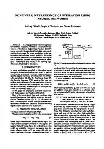
numerical methods, like finite element method (FEM), which transforms the electromagnetic interference problem into a numerical one [2]. Although FEM yielded solutions are very accurate, regarding to the problem complexity, the computing time of this method increases with the geometry, its mesh, material characteristics and requested evaluation parameters. The study of electromagnetic interference between HVPL and MP with FEM for different system configurations requires expensive computing time because, for each new problem geometry taken under consideration FEM involves a new mesh and new calculations. Therefore, a scaling method of the results from one configuration case to another may be of interest if it provides less computing time. To decrease the computing time, needed to study new problem geometries, an artificial intelligence based method, a neural network (NN) solution, is proposed by the authors. To identify the optimal neural network solution different architectures were implemented and tested. Obtained results were compared to FEM solutions, considered standard ones. 2. ELECTROMAGNETIC INTERFERENCE PROBLEM The authors purpose is to evaluate the magnetic vector potential (MVP), induced on the MP for an electromagnetic interference problem presented in [4, 5]. The problem, presented in Fig. 1, refers to an underground metallic gas pipeline which shares for 25 km the same distribution corridor with a 145 kV HVPL at 50 Hz frequency.

Fig. 1 – Top view of the parallel exposure.

It is assumed that a phase to ground fault occurs at point B, far away outside the common HVPL–MP distribution corridor. The earth current associated with this fault has a negligible action upon the buried pipeline. This fact allows us to

164

Dan D. Micu et al.

3

assume only an inductive interference caused by the flowing fault current in the section where the HVPL runs parallel to the buried gas pipeline. The HVPL consists of two steel reinforced aluminium conductors per phase. Sky wire conductors have a 4 mm radius, the gas pipeline has a 0.195 m inner radius, a 0.2 m outer radius and a 0.1 m coating radius. The characteristics of the materials in this configuration have the following properties: the soil is assumed to be homogeneous; MP and sky wires have an σ = 7.0E+05 S/m conductivity and a µr = 250 relative permeability [4]. End effects are neglected, leading to a two dimensional (2D) problem which depends on the separation distance d between HVPL and MP, on the soil resistivity ρ, on the x and y coordinates of the point where the magnetic vector potential is desired to be determined. Figure 2 shows the studied configuration cross section:

Fig. 2 – Cross section of the system taken under investigation.

Thus, taking into account the cross section of the studied problem, the z direction component of the magnetic vector potential Az and of the total current density Jz are described by the following system of equations:

 1   µ 0µ r     

 ∂2 A ∂2 A  ⋅  2z + 2z  − jωσAz + J sz = 0 ∂y   ∂x − jωσAz + J sz = J z

(1)

∫∫ J ds = I , z

i

Si

where σ is the conductivity, ω is the angular frequency, µ0 is the permeability of the free space (µ0 = 4·π·10-7 H/m), µr is the relative permeability of the

4


165

environment, Jsz is the source current density in the z direction and Ii is the imposed current on conductor i of Si cross section. To solve the system (1) for a given problem geometry (HVPL-MP separation distance, soil resistivity) with FEM, it takes from 20 to 50 minutes depending on mesh discretization. This computing time has to be repeated for each problem geometry (soil resistivity/separation distance) that we want to study. In order to eliminate the computational time needed to evaluate MVP values for each problem geometry, the authors implemented a neural network solution to scale the MVP values for a set of known problem geometries. 3. NEURAL NETWORK CONCEPTS Neural Networks (NN) belong to a group of artificial intelligence techniques (AI), for data analysis that do not resemble with other classical analysis techniques. AI is learning about the chosen subject from the data provided to them, rather than being defined by user. NN get their knowledge by detecting relationships between input and output data [6]. A. Structure of an artificial neuron The most complex neural network in nature is the human brain. This inspired scientists in designing artificial neural networks. Like in nature, the major building block of any neural network is the artificial neuron.

Fig. 3 – Structure of a: a) biological neuron; b) artificial neuron.

The artificial neuron like the biological one (Fig. 3) is a system which has a variable number of inputs u k , k = 1, m (dendrites) and only one output y (axon). The inputs of the artificial neurons are multiplied by some wk parameters, called weighs and added to each other. The weighted inputs sum is added to a parameter b called bias [7]. Then the last sum, denoted by h , is used as an argument of the function which produces the artificial neurons output. This function is called transfer function and can take various forms, specific to each neuron. This is the

166

Dan D. Micu et al.

5

equivalent to nucleus of the biological neuron. Thus the artificial neurons output is described by the following relation: m

y = f a (h), where h = ∑ (u k ⋅ w k ) + b .

(2)

k =1

B. Neural network structure A group of artificial neurons, which work in parallel, their inputs and outputs have the same destination from a layer. Each neural network must contain at least one layer of neurons, but can join as many as someone projects. The layer gathering the neurons which give the neural networks output is called output layer. Layers which contain the neurons interposed between the global inputs of the neural network and the inputs of the neurons from the output layer are called hidden layers [8]. Usually, there are used feed-forward NN which contain a hidden layer and an output layer. Figure 4 presents the simplified block diagram of a two layer feed-forward neural network.

Fig. 4 – Feed-forward neural network.

From this block diagram, it can be deduced the relation which defines a feedforward NN outputs, if we know its inputs uk , k = 1, m . The hidden layer neurons output is described by the following relation:

 ν j = f a1 h1j = f a1  

( )

∑ (u

k

k

 ⋅ wkj ) + b1j  . 

(3)

So, the final outputs of a feed-forward neural network will be given by:

 y i = f a 2 hi2 = f a 2   

( )

∑ (w j

kj

 ⋅ f a1 h 1j + b 2j  .  

( ))

(4)

6


167

C. Training a neural network Training of a neural network is the process in which it is taught to provide the desired output values.

Fig. 5 – Feed-forward neural network.

According to the Fig. 5, NN weights are adjusted depending on the error between the actual NN outputs and the desired ones. This error is evaluated by a performance function. In most of the cases the mean square error is used as performance function:

E=

1  n * yi − yi ⋅ n  i =1

∑(

)  . 2



(5)

4. NEURAL NETWORK IMPLEMENTATION In order to determine precisely the magnetic vector potential, in each point of the studied domain, the amplitude and the phase of MVP has to be evaluated. To obtain more accurate results, considering the different variation range of these to values: 10-6 ÷10-4 [Wb/m] for amplitude, and respectively –180°÷180° for phase, the authors chose to implement two different neural networks – one for amplitude and one for phase – instead of implementing a single NN which provide both amplitude and phase. These two NN have as input values the parameters which describe the presented 2D problem: • d – separation distance between HVPL and MP (between 10 m and 2000 m); • ρ – the resistivity of the soil (between 30 Ω·m and 1000 Ω·m); • x, y – coordinates of the point where the MVP will be evaluated. To implement the proposed two NN it was used the Neural Networks toolbox from MatLab software. This software was chosen because it enables the creation of almost all types of NN from perceptrons (single layer networks used for classification) to more complex architectures of feed-forward or recurrent networks. In order to create a feed-forward neural network in MatLab the following function has to be used:

168

Dan D. Micu et al.

7

net = newff(P,T,S,TF,BTF,BLF,PF), where: • • • • • • •

(6)

P – is a RxQ1 matrix of Q1 representative R-element input vectors; T – is a SNxQ2 matrix of Q2 representative SN-element target vectors. S – is a vector representing the number of neurons in each hidden layer; TF – is a vector representing the transfer function used for each layer; BTF – is the back propagation function used to train the NN; BLF – is the weight/bias learning function; PF – is performance evaluation function.

In order to find the optimal NN solutions to evaluate the amplitude and phase of MVP different NN architectures were implemented. A basic feed-forward NN architecture with one hidden layer and one output layer has been chosen. The number of neurons in the hidden layer was varied from 5 to 30 with a step of 5 neurons. The transfer function of the output layer was set to purelin (the linear transfer function) and the transfer function on the hidden layer was varied between tansig (the hyperbolic tangent sigmoid transfer function), logsig (the logarithmic sigmoid transfer function and purelin. Also performance evaluation function was varied between mse (mean square error), msereg (mean square error with regularization performance) and sse (sum squared error). To train the different NN architectures the Levenberg-Marquardt training method and the descendent gradient with momentum weight learning rule has been implemented. As training data base a set of MVP values evaluated with FEM and presented in [4] were used. These MVP values were calculated in different points up to 15 different problem geometries (soil resistivity/separation distance) obtaining a set of 37 input/output pairs used to train the proposed NN. Table 1 presents some of the training data. Table 1 Input/Output pairs used to train the proposed NN No 1 5 9 14 18 23

x

y

[m]

[m]

[m]

70 800 400 70 1000 300

70 818.25 384.81 40 1022.5 290.26

d

-15 -13.5 -7.82 0 0 -15.8

ρ [Ωm] 30 30 70 100 100 500

MVP Ampl. Phase 10-3 [º] [Wb/m] 36.1 -22.8 3.88 -82.61 17.2 -44.46 55.9 -18.53 7.23 -67.27 35.5 -26.74

8

Neural networks applied in electromagnetic interference problems 28 30 33 37

700 150 1500 2000

670 150.55 1499.1 2030

-22.5 -16.99 -17.48 -5

700 900 900 1000

26 53 15.6 12.2

169

-33.74 -19.7 -46.35 -52.73

To obtain a higher accuracy for the results given by the two neural networks, the training database presented in [4] was multiplied twenty times. The training process for both amplitude and phase neural networks took from 10 seconds to 1 minutes, depending on NN architecture. Once the NN are trained they can provide automatically the amplitude, respectively the phase of MVP for any combination of input data. To obtain the output value, given by an implemented NN, the following MatLab function has be used: sim(NET,X,T),

(7)

where: NET – is the implemented neural network; X – is a R × Q1 matrix of Q1 representative R-element input vectors; T – is a SN × Q1 matrix of Q1 representative SN-element target vectors. In order to identify the optimal NN architecture for both amplitude and phase, and see how these react in the presence of totally new problem geometries, the implemented NN were tested by providing as input values the database presented in Table 2. The obtained results were compared with MVP values obtained with FEM calculation. Table 2 Input/Output pairs used to train the proposed NN No 1 2 3 4 5 6 7 8

d [m] 70 70 400 300 700 1000 1000 1500

x

y

[m]

[m]

40 81.66 392.25 281.66 690.36 1007.50 1015 1524.77

-15 -27.03 -25.56 -27.03 -15.80 0 -30 -6.93

ρ [Ωm] 100 30 70 500 700 70 100 900

MVP Ampl. 10-3 [Wb/m] 53.8 32.90 16.7 37.5 25.6 5.68 7.16 15.40

Phase [º] -19.34 -25.57 -46.05 -25.93 -34.07 -72.98 -69.22 -46.56

After analysing maximum and average percentage error, between the obtained results as output values of the implemented NNs and results obtained with FEM calculation for both testing and training data sets, the authors had chosen the optimal NN architectures.

170

Dan D. Micu et al.

9

In case of the NN which calculates the amplitude, the optimal NN architecture it would be a feed-forward NN with 10 neurons and tansig transfer function on the hidden layer, respectively a mean square error function used for performance evaluation. This optimal NN architecture register a maximum error of 1.72% and average error of 0.71% for the testing data set; all the other tested NN architectures percentage average errors are grater than 2%. Figure 6 presents the absolute deviation between the results obtained with the optimal NN architecture and those calculated with FEM for the testing data set.

Fig. 6 – Absolute deviation for optimal amplitude NN.

In case of NN which calculates the phase, the optimal architecture it would be a feed-forward NN with 5 neurons and logsig transfer function on the hidden layer, respectively a sum square error function used for performance evaluation. This optimal NN architecture presents a maximum error of 5.47% and average error of 1.54% for the testing data set; all the other tested NN architectures percentage maximum error are grater than 10%. Figure 7 presents the absolute deviation between the results obtained with the optimal NN architecture and those calculated with FEM for the testing data set.

Fig. 7 – Absolute deviation for optimal phase NN.

10


171

5. CONCLUSIONS The authors have proposed the use of an artificial intelligence technique to scale the MVP values for any geometrical configuration for a specific electromagnetic interference problem, from a set of known problem geometries, in order to reduce computation time for new problem configurations.From figure 6 and 7 it can be observed that absolute deviation of the solutions provided by the identified optimal NN architectures, are almost insignificant for both the amplitude and phase NN, to those provided by FEM. The method using neural networks, implemented for the MPV evaluation for different geometrical configurations, is a very effective one, especially if we take into account the fact that the solutions provided by neural networks are obtained instantaneously and we do not have to pay expansive calculus as with FEM. ACKNOWLEDGMENTS The authors are grateful to the Romanian Ministry of Scientific Research and Technology, for the financial support in the frame of the TE_253/2010_CNCSIS project “Modeling, Prediction and Design Solutions, with Maximum Effectiveness, for Reducing the Impact of Stray Currents on Underground Metallic Gas Pipelines”, No. 34/2010. Also the paper was supported by the project "Doctoral studies in engineering sciences for developing the knowledge based societySIDOC” contract no. POSDRU/88/1.5/S/60078, project co-funded from European Social Fund through Sectorial Operational Program Human Resources 2007-2013. Received on February 15, 2011

REFERENCES 1. F. Dawalibi, Analysis of electrical interference from power lines to gas pipelines. Part I –Computation methods, IEEE Trans. on Power Delivery, 4, 3, pp. 1840-1848 (1989). 2. Dan D. Micu, I. Lingvay, C. Lingvay, L. Darabant, A. Ceclan, Numerical evaluation of induced voltages in the metallic underground pipelines, Rev. Roum. des Sci. Techn. – Électrotechn. et Énerg., ISI Journal, 54, 2, pp. 175-184 (2009). 3. * * *, Guide Concerning Influence of High Voltage AC Power Systems on Metallic Pipelines, CIGRE Working Group 36.02, Canada, 1995. 4. K. J. Satsios, D. P. Labridis, P. S. Dokopoulos, An Artificial Intelligence System for a Complex Electromagnetic Field Problem: Part I – Finite Element Calculations and Fuzzy Logic Development, IEEE Trans. on Magnetics, 35, 1, pp. 516-522, 1999. 5. K. J. Satsios, D. P. Labridis, P. S. Dokopoulos, An Artificial Intelligence System for a Complex Electromagnetic Field Problem: Part II – Method Implementation and Performance Analysis, IEEE Trans., 35, 1, pp. 523-527 (1999). 6. S. Al-Badi, K. Ellithy, S. Al-Alawi, Prediction of Voltages on Mitigated Pipelines Paralleling Electric Transmission Lines Using an Arificial Neural Network, The Journal of Corrosion Science and Engineering, 10 (2007). 7. M. Caudil, C. Butler, Understanding Neural Networks: Computer Exploration, Vol. 1 & Vol. 2, MA: MIT Press, Cambridge, 1992. 8. H. Demuth, M. Beale, Neural Networks Toolbox. Users’ Guide, Ver. 3. The MATHWORKS Inc., 1998.