Neural Networks Based Colour Measuring for Process Monitoring and ...

Neural Comput & Applic (2000)9:227–242  2000 Springer-Verlag London Limited

Neural Networks Based Colour Measuring for Process Monitoring and Control in Multicoloured Newspaper Printing A. Verikas1,2, K. Malmqvist1, and L. Bergman1 1

Intelligent Systems Laboratory, Halmstad University, Halmstad, Sweden; 2Department of Applied Electronics, Kaunas University of Technology, Kaunas, Lithuania

This paper presents a neural networks based method and a system for colour measurements on printed halftone multicoloured pictures and halftone multicoloured bars in newspapers. The measured values, called a colour vector, are used by the operator controlling the printing process to make appropriate ink feed adjustments to compensate for colour deviations of the picture being measured from the desired print. By the colour vector concept, we mean the CMY or CMYK (cyan, magenta, yellow, and black) vector, which lives in the three- or fourdimensional space of printing inks. Two factors contribute to values of the vector components, namely the percentage of the area covered by cyan, magenta, yellow and black inks (tonal values) and ink densities. Values of the colour vector components increase if tonal values or ink densities rise, and vice versa. If some reference values of the colour vector components are set from a desired print, then after an appropriate calibration, the colour vector measured on an actual halftone multicoloured area directly shows how much the operator needs to raise or lower the cyan, magenta, yellow and black ink densities to compensate for colour deviation from the desired print. The 18 months experience of the use of the system in the printing shop witnesses its usefulness through the improved quality of multicoloured pictures, the reduced consumption of inks and, therefore, less severe problems of smearing and printing through. Correspondence and offprint requests to: A. Verikas, Centre for Imaging Sciences, Halmstad University, S-30118 Halmstad, Sweden. Email: antanas.verikas얀ide.hh.se

Keywords: Colour classification; Colour printing; Decision fusion; Graphic arts; Neural networks

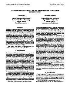
1. Introduction Multicoloured pictures in newspapers are most often created by printing dots of cyan (C), magenta (M), yellow (Y) and black (K) inks upon each other through screens having different raster angles. Figure 1 illustrates an example of an enlarged view of a small area of a newspaper picture that contains dots of all of the four inks. A key factor in high quality multicolour printing of pictures is to measure and control the amount of the four inks transferred to the paper. This paper deals with the measurement

Fig. 1. An enlarged view of a part of a newspaper picture that was created by printing dots of cyan, magenta, yellow and black inks.

228

of the amount of inks and generation of signals for controlling the amounts. Nowadays, the usual way to obtain the quantitative values for controlling the amount of inks in newspaper printing is by measuring the ink densities in specific printed test areas in the newspaper, for example in a colour bar, as shown in Fig. 2. The publisher seldom accepts such test areas. Besides, such measurements are indirect and hard to handle for the operator controlling the printing process. The operator is faced with a hard task of deciding how to change the densities of the four inks in order to improve the quality of pictures. This often leads to over-inked printing. The over-inked printing results in higher costs for inks, as well as serious problems of smearing and printing through. By measuring solid print ink densities, an operator can only obtain very fuzzy information about how to control the printing process. This can easily result in attempts to correct the printing process by increasing ink densities, in spite of the fact that the process is already running in the over-inked phase. Moreover, measuring the solid print density does not take into consideration the effect of dot gain and light scattering that appear in a multicoloured screen area. The right consideration of these phenomena has crucial importance for achieving a high quality of halftone multicoloured prints in newspapers. The operator would feel much more secure having an instrument, instead of a densitometer which, when placed on a multicoloured picture, would show how much he or she needs to increase/decrease the amount of cyan, magenta, yellow and black inks, if compared with some reference pre-print. In the case of measuring in an arbitrary part of a picture, a positioning problem may occur when comparing the measured values with the reference values taken from the reference pre-print. However, double greybars that are widely used in newspaper printing in Sweden and other countries as well, suit well for that purpose. One half of the double grey-bar is printed with the three inks cyan, magenta and yellow, while the other half is printed as a black

Fig. 2. Example of a colour bar containing cyan, magenta, yellow, and black colours.

A. Verikas et al.

halftone screen, as shown in Fig. 3. Such double grey-bars are easily hidden from a reader by printing them as a double grey-line, for example. Another important tool printing shops lack today is an instrument providing the possibility to examine the picture obtained at a microscopic level, and compare the picture with the desired result. By examination at a microscopic level, we mean an inverse colour separation of an image taken from the printed picture and an examination of the printed result obtained separately for each ink used. This would give a better understanding of the interaction of different types of paper, ink and printing devices. Achieving colourimetric reproduction from a printing device typically involves two steps. First, the printing device is characterised by identifying a mapping that relates the device-dependent input signals, for instance C, M, Y and K, to the colour of resulting printed patch, usually specified in a deviceindependent colour space such as L*a*b*. Secondly, a colour error correction transform is derived. The error correction transform is essentially an inverse of the characterisation mapping. The transform maps the colour specification in the device independent colour space to the C, M, Y and K ink amounts required to obtain the specified colour. Characterisation of the printing device, colour error correction, as well as trans-media colour matching, are the main problems in colour reproduction. Characterisation of printing device and colour correction are often complex non-linear transformations, which are derived from numerous measurements or models of a printing device. The derived transformations are usually folded into lookup tables. Among the sources of errors in these transforms are inaccuracies in lookup table approximations, noise in the data, inaccuracy in the model of the printing device, and the limited number of data used. The errors

Fig. 3. An example of a double grey-bar.

Colour Measuring for Process Monitoring and Control

limit the final accuracy of the transforms. Moreover, characteristics of the printing device often drift over a period of time. Thus re-characterisation, and therefore more measurements, are required. A printing device is most often characterised by using the optimised spectral Neugebauer model [1,2]. The least squares, the weighted least squares, and the total least squares regression methods are the main techniques used to estimate parameters of the model [1,2]. Since the characterisation, colour correction and matching transformations do not readily lend itself to linear mathematical solutions, there is a need to use other techniques, which are capable of nonlinear modelling. Artificial neural networks have proved themselves to be capable of discovering complex mapping functions using powerful learning algorithms. In colour research, artificial neural networks have been used for discovering transformations between different colour spaces [3,4], colour gamut mapping [5], cross-media colour matching [6], calibrating spectrophotometers [7,8], and colour error reduction in television receivers [9]. In this project, we use artificial neural networks for colour measuring on halftone multicoloured pictures in newspapers. The values obtained are used by the operator controlling the printing process to make appropriate ink feed adjustments to compensate for colour deviations of the picture being measured from the desired print. In this paper, we present a method and a tool for colour measurements directly on printed halftone multicoloured pictures, including the double greybars, as well as for inverse colour separation. Assuming the reference print is provided, a double grey-bar, for example, the developed measuring device when placed on an actual double grey-bar directly shows how much the operator needs to raise or lower the cyan, magenta, yellow and black ink densities in order to correct colours of the double grey-bar being measured. We introduce the concept of colour impression [10,11]. By this we mean the CMY or CMYK vector (colour vector), which lives in the three- or four-dimensional space of printing inks. Two factors contribute to values of the vector components, namely the percentage of the area covered by cyan, magenta, yellow and black inks (tonal values) and ink densities. The values of the components are obtained by registering the RGB image from the measuring area, transforming the RGB image to its L*a*b* counterpart, and then mapping the set of the average L*a*b* values for the area to the triplet or quadruple of CMY or CMYK, respectively. We use artificial neural networks to learn and perform the mapping L*a*b*

229

→ CMY(K). The procedure of the inverse colour separation is involved when learning the mapping. By inverse colour separation, we mean the decomposition of the RGB image into nine binary images, namely, ‘White image’, ‘Cyan image’, . . ., ‘Green (CY) image’, . . ., ‘CMY image’ and ‘Black (K) image’. Values of all pixels of the White image are equal to zero, except those corresponding to the areas of the picture that have not got any ink during the printing process. Values of such pixels are equal to one. Accordingly, values of pixels collected into the Green (CY) image are set to one if they correspond to the areas of the picture printed with both cyan and yellow inks. The meaning of the other types of binary images is straightforward. Based on the separation results the C, M, Y and K values (the percentage of the area covered by the different inks) are easily estimated and used as targets for learning the mapping L*a*b* → CMY(K). We note that such an inverse colour separation is valuable not only as an auxiliary tool for performing the transformation from L*a*b* to CMY, but also on its own, since it provides a possibility to inspect the printing result. We use algorithms based on artificial neural networks for performing the inverse colour separation. A detailed description of the algorithms can be found elsewhere [12,13]. The colour vector expresses integrated information about the tonal values and ink densities. This is a valuable property, since we never know exactly what actual tonal values we will obtain. Values of the colour vector components increase if tonal values or ink densities rise, and vice versa. If, for some primary colour, ink density and tonal value do not change, the corresponding component of the colour vector remains constant. Such a behaviour of the colour vector makes it much easier for the operator to adjust the printing process. If some reference values of the colour vector components are set from a pre-print, then the colour vector directly shows how much the operator needs to raise or lower the cyan, magenta, yellow and black ink densities in order to compensate colour deviation of the picture being measured. During the experimental investigations, we have found a good correlation between components of the colour vector and ink densities. The rest of the paper is organised as follows. In the next two sections we briefly describe the concept of colour impression and the tools used. Section 4 presents the colour space used. The method for inverse colour separation is briefly described in Section 5. Section 6 presents a method for accomplishing the transformation from the set of L* a*b* values to the colour vector. Section 7 summar-

230

A. Verikas et al.

ises the results of experimental investigations. Finally, Section 8 presents conclusions of the work.

2. The Concept of Colour Impression Colour impression of a printed picture depends both upon actual tonal values and ink densities. By actual tonal values we mean the nominal tonal values ⫹ the mechanical dot gain ⫹ the optical dot gain. The most common reason for the mechanical dot gain is that the viscosity of the ink cannot be high enough to avoid some spreading when the dot has been deposited on the blanket. There are two types of optical dot gain. The first type is dependent on the frequency response of the human eye, while the other type of optical dot gain is caused by the substrate, as most of the light reaching the paper surface penetrates into it, scatters and later emerges through the top and bottom surfaces. An operator controlling the printing process never knows the actual tonal values and controls the process by adjusting densities of inks. This is not an easy task for the operator, since it is not clear how big adjustments should be made for cyan, magenta, yellow and black, respectively. The degree of adjustments needed may depend upon the type of paper and inks, humidity, the duration of the printing process and other factors. The reason for introducing the concept of the

colour vector of colour impression is to integrate information from both actual tonal values and ink densities, and to show how much an operator controlling the printing process needs to raise or lower the cyan, magenta, yellow and black ink densities, in order to compensate the colour deviation of a picture being measured in reference to some preprint. Figure 4 shows the main window of the colour impression software. The components of the colour vector are shown on the right-hand side of the window as colour bars. There are five measurements shown in Fig. 4. One measurement, shown as a column of colour bars in the figure, stands for one set of ink keys controlling ink feed in a printing press. The five measurements shown are taken from one newspaper page having five sets of ink keys each. There is a space reserved for visualising two such pages in the main window. On the left-bottom part of the figure the history of the measurements is shown for the magenta colour. Values of the colour vector components range between 0 and 100. The black strips on the colour bars indicate values of the colour vector components measured on some reference picture, for example on a double grey-bar. Having this information the operator can see exactly how the feeds of inks should be changed. For example, in the figure, the adjustments need to be performed to eliminate the colour deviations are shown in relative units bellow the colour bars. The

Fig. 4. The main window of the colour impression software.

Colour Measuring for Process Monitoring and Control

231

left-upper part of the window displays the image used to calculate the colour vector components. When using a double grey-bar the ‘black’ component of the colour vector is measured on the part of the bar printed as a black halftone screen. The CMY components of the colour vector are measured on the opposite half of the bar. Both measurements are made at the same time.

3. Tools and Data The equipment we use consists of a measuring device, a frame-grabber, a PC and software. For the image acquisition a specially designed measuring device was developed consisting of a one-chip CCD colour camera and six photo diodes as the light source. The resolution used was such that an image consisting of 512 ⫻ 512 pixels was recorded from an area of 5 ⫻ 8 mm2. All pictures we used were printed on an ordinary newsprint paper of approximately 45 g/m2 weight. All the input/output signals of the neural networks are normalised to fall into the interval [0,1]. The use of a CCD colour camera for measuring colour prints can be a point of contention. However, note that we make only relative comparisons when measuring on colour prints. Besides, the device we developed is tuned to a customer’s data set during the training process as it is explained in the following sections.

4. Colour Space Used In general, colours differ in both chromaticity and luminance. A method of combining these variables is required in order to measure the difference between colours. Colour image acquisition equipment such as a CCD colour camera obtains the RGB values, which can be directly used for representing colours in the RGB colour space {R,G,B} ⫽

冕

E(␭)O(␭)F(␭)d␭

(1)

where E(␭) expresses spectral properties of the illumination source, O(␭) is spectral reflectance function of an object, and F(␭) stands for three spectral sensitivity functions of the colour camera. However, different acquisition equipment gives us different RGB values for the same incident light. One more drawback of the RGB colour space is that the metrics does not represent colour differences in a uniform scale, making it difficult to evaluate

the similarity of two colours from their distance in the space. To meet the requirement of uniformity of distribution of colours the Commission Internationale de l’Eclairage (CIE) has recommended using one of two alternative colour spaces: L*u*v* or L*a*b* colour space [14,15]. It is a common practice to use the L*a*b* colour space for describing absorbing materials such as pigments and dyes. Therefore, we used the L*a*b* colour space in all procedures that involve colour distance calculations and colour transformations. However, when performing the inverse colour separation we use the colour space based on colour difference signals, the definition of which will be given shortly. To map the RGB values into the L*a*b* colour space, the RGB values are first transformed to the XYZ tristimulus values as follows: X ⫽ a11R ⫹ a12G ⫹ a13B

(2)

Y ⫽ a21R ⫹ a22G ⫹ a23B

(3)

Z ⫽ a31R ⫹ a32G ⫹ a33B

(4)

with the coefficients aij being determined by a colourimetric characterisation of the hardware used. XYZ tristimulus values can describe any colour. It is often convenient to discuss ‘pure’ colour in the absence of luminance. For that purpose, the CIE defines x and y chromaticity co-ordinates: x⫽

X X⫹Y⫹Z

(5)

y⫽

Y X⫹Y⫹Z

(6)

A colour plots as a point in an (x,y) chromaticity diagram. However, the distribution of colours observed in the (x,y) chromaticity diagram is also non-uniform. A dominant wavelength correlates very non-uniformly with the perception of hue and excitation purity with the perception of saturation. Having XYZ tristimulus values the L*a*b* colour space is defined as follows [14]: L* ⫽ 116(Y/Yn)1/3 ⫺ 16, if Y/Yn ⬎ 0.008856 (7) L* ⫽ 903.3(Y/Yn), if Y/Yn ⱕ 0.008856

(8)

a* ⫽ 500[X/Xn)

⫺ (Y/Yn) ]

(9)

b* ⫽ 200[(Y/Yn)1/3 ⫺ (Z/Zn)1/3]

(10)

1/3

1/3

where Xn,Yn,Zn are the tristimulus values of X,Y and Z for the appropriately chosen reference white. If any of the ratios X/Xn, Y/Yn and Z/Zn is equal to or less than 0.008856, it is replaced in the above formulae by:

232

A. Verikas et al.

7.787f ⫹ 16/116

(11)

where f is X/Xn, Y/Yn or Z/Zn, as the case may be [14]. New measures are provided in the colour space which correlate with hue and saturation more uniformly. For example, CIE hue-angle Hab [14]: Hab ⫽ arctan(b*/a*)

(12)

The Euclidean distance measure can be used to measure the distance (⌬E) between the two points representing the colours in the colour space: ⌬E*ab ⫽ [(⌬L*)2 ⫹ (⌬a*)2 ⫹ (⌬b*)2]1/2

(13)

We use the colour space based on the colour difference signals f1, f2 and f3 when performing the inverse colour separation. The task of the colour separation is to assign each pixel of an image being analysed into one of nine colour classes as it is explained in the next section. Note that we do not measure any colour distances for accomplishing the inverse colour separation. If we assume the random variables R, G and B to be of equal variances (␴2) and covariances (only variances of the variables have been normalised to be equal to one in our experiments), the covariance matrix of these variables can be written as:

冘

冤冥 1rr

⫽␴

2

r1r

(14)

rr1

where r is the correlation coefficient. The eigensolution of the covariance matrix gives the following eigenvectors (ei): e1 ⫽ {1,1,1}t, e2 ⫽ {1,0,⫺1}t, e3 ⫽ {1,⫺2,1}t and the corresponding eigenvalues (␭i): ␭1 ⫽ ␴2(1⫹2r), ␭2 ⫽ ␭3 ⫽ ␴2 (1⫺r), where t means a transpose. The linear transform of the {R,G,B} vector by the eigenvectors produces other random variables f1, f2 and f3: f1 ⫽ R ⫹ G ⫹ B, f2 ⫽ R ⫺ B, f3 ⫽ R ⫺2G ⫹ B, which are almost uncorrelated. The choice of the f1 f2 f3 colour space was based on experimental testing. Five colour spaces, namely, RGB, HSI, CIELuv, CIELab and f1 f2 f3 have been tested in the inverse colour separation and compared experimentally. The f1 f2 f3 colour space provided the highest classification accuracy [12,13]. Moreover, the linear transformation RGB → f1 f2 f3 is much faster to perform than the non-linear one RGB → L*a*b*.

5. Inverse Colour Separation We perform the inverse colour separation by determining the colour of every pixel of the image

taken from a printed picture. Hierarchical modular neural networks are used for solving the colour classification task. When mixing dots of cyan, magenta and yellow colours, eight combinations are possible for each pixel in the picture. The combination CMY produces the black colour. However, in practice, black ink is most often also printed. We assume the black ink to be opaque and therefore C⫹K ⫽ M⫹K ⫽ Y⫹K ⫽ C⫹M⫹Y⫹K ⫽ K. Therefore, we have to distinguish between nine colour classes, namely C, M, Y, W (white paper), CY, CM, MY, CMY (black resulting from overlay of cyan, magenta, and yellow) and K (black resulting from black ink or black ink plus any other component). The variables f1, f2 and f3 serve as input to the colour classification neural network. To achieve an acceptable classification error and a high average classification speed we use a hierarchical committee of neural networks [12,13]. The committee solves the classification task in two stages. In the first stage, each pixel is assigned to one of six clusters of colours, namely, {C}, {W}, {Y}, {CY}, {M,MY} and {CM,CMY,K}. In the second stage, the clusters {M,MY} and {CM,CMY,K} are further divided. We use this approach since the colours {M,MY} and {CM,CMY,K} form two clusters of highly similar colours when pictures of newspaper printing quality are considered. In addition to the variables f1, f2 and f3, we extract some features (minimum, maximum, average values of the variables f1, f2 and f3) from the surroundings of the pixel being analysed when classifying pixels from these clusters of similar colours. See elsewhere [12,13] for details on the classification procedure.

6. Transformation from L*a*b* to CMY We consider two versions of the required mapping L*a*b* → CMY(K). Assuming that double grey-bars are used as measuring areas, two separate mappings, namely L*a*b* → CMY and L*a*b* → K are learned. We use the first mapping to obtain the CMY values for the coloured part of the double grey-bar, and the second one for getting the K value for the black part of the bar. Measuring on arbitrary areas of CMYK pictures requires the mapping L*a* b* → CMYK, which is not unique since different CMYK signals may yield same L*a*b* values. As suggested by Tominaga [16], we solve this problem by learning the mapping in two steps, as shown in Fig. 5. In the first step, the neural network B is trained to learn the mapping CMYK → L*a*b*. The network’s B weights are then frozen, and the identity

Colour Measuring for Process Monitoring and Control

233

Fig. 5. Network structure for determining mapping CMYK → L* a*b*. Fig. 6. A general structure of the transformation network.

mapping L*a*b* → L*a*b* is learned by optimising weights of the network A in the concatenated structure. After convergence, the network A is ready to perform the desired mapping L*a*b* → CMYK. 6.1. Structure of the Transformation Network Artificial neural networks can learn complex mapping functions, however, they are unstable to perturbations in a learning set. The sensitivity of neural networks to a composition of the learning set may cause serious problems when learning sets are small and rather noisy. This is the case in our application, since to make the colour measuring approach be easy manageable in practice, we use quite small training sets. Besides, the training sets are rather noisy since in newspaper printing it is still hard to achieve a high quality printing result. To cope with the neural networks stability problem we use Bayesian regularisation [17,18] and committees of neural networks for learning the desired mappings. It is well known that regularisation as well as a combination of many different estimators can improve the accuracy of the estimate for unseen data. We use a neural networks committee of the type presented in Fig. 6 for learning each of the mappings L*a*b* → CMY, L*a*b* → K and L*a*b* → CMYK. Each member of the committee is a two hidden layer perceptron and performs the same task. All the hidden nodes of the members of the committees possess sigmoidal transfer functions while the output nodes are linear. The outputs of the members of the committee are then combined to obtain the committee output. By using two hidden layers we obtained a more efficient approximation in the sense of achieving the same level of accuracy with fewer weights in total than in the one hidden layer case.

This is probably to the fact that neurons of a single hidden layer tend to interact with each other globally, and this interaction makes it difficult to improve the approximation at one point without worsening it at some other point [19]. 6.2. Combining Answers of Committee Members A variety of schemes have been proposed for combining multiple estimators. The most often used approaches include: average [20,21], weighted average [22–26], selection of the best in some region of the input space [27], fuzzy integral [28,29], and the Dempster-Shafer theory [30]. See Verikas et al. [31] for a comparative study of different combination schemes. We can say that a combiner assigns relative weights of importance to estimators in one way or another. The weights can be data dependent [31,32], or can express the worth averaged over the entire space [22,23]. The use of data dependent weights, when properly chosen, provides a higher accuracy of the estimate [31]. In this work, we integrate two methods, namely, a weighted average and the selection of the best in some region of the input space when combining outputs of the committee members. Let yi(x) denote the actual output of the ith member of the committee. A weighted combination of outputs of a set of L networks (a committee output) can then be written as

冘␭ L

y(x) ⫽

i

i⫽1

(x)yi(x)

(15)

234

A. Verikas et al.

where the weights ␭i(x) need to be determined. Note that the weights depend upon x. To estimate the weights, we first distribute a number Nrf of reference points mi in the colour space and determine the prediction error for each member of the committee in the neighbourhood of every reference point. The reference points are distributed by performing the frequency-sensitive competitive learning [31]. The average squared prediction error for the ith member in the neighbourhood of the jth reference point can be written as eij ⫽ E{储yi(x) ⫺ t(x)储2}

(16)

where t(x) is the target output vector and E{·} denotes the expectation calculated in the neighbourhood of the jth reference point. In the experimental tests presented in this paper, we calculated the average empirical error instead of the expected error. The weight of the ith committee member in the neighbourhood of the jth reference point is given by

␭ij ⫽

exp(⫺␩ eij)

冘 L

(17)

exp(⫺␩ eij)

i⫽1

where ␩ is a constant. Since the weights ␭ij can be different in various regions of the colour space, we say that the weights ␭i depend upon x. Now, given input x, the output of the committee is determined in two steps. First, the nearest reference point k is found: k ⫽ arg

min

d(x,mi)

(18)

i⫽1,. . .,Nrf

where d(x,mi) is the distance between vectors x and mi. Then the output of the committee is given by

冘␭ L

y(x) ⫽

(x)yi(x)

ik

(19)

i⫽1

6.3. Training Committee Members Numerous previous works on neural networks committees have shown that an efficient committee should consist of networks that are not only very accurate, but also diverse, in the sense that the networks make their errors in different regions of the input space [33–35]. One way to increase the diversity is to use special sampling techniques for collecting learning sets to train committee members. Bootstrapping [36,37], Boosting [38] and AdaBoosting [39,40] are the most often used approaches for data sampling when training members of neural network committees. Boosting is a complex tech-

nique compared to bootstrapping. Some studies show that boosting may create committees that are less accurate than a single network [41]. Boosting may suffer from overfitting in the presence of noise [41,42]. In our application, data sets are rather noisy. Therefore, we have chosen the bootstrapping sampling technique. We train each member of the committee by minimising the following objective function:

␤ E ⫽ ␤ED ⫹ ␣Ew ⫽ 2 ⫺ tnk}2 ⫹

␣ 2

冘

冘冘 ND

Q

{yk(xn;wi)

(20)

n⫽1 k⫽1

Niw

(wij)2

j⫽1

where xn stands for the nth input data point, ND is the number of input data, Q is the number of outputs in the network, wi is the weight vector of the ith member, Niw is the number of weights in the ith member of the committee, and ␣ and ␤ are objective function hyper-parameters. The second term of the objective function performs regularisation. We use the Levenberg–Marquardt algorithm for neural network training [43] and Bayesian techniques to optimise regularisation [18,44]. In the Bayesian approach, the weights of the network are considered as random variables. Once we observe the data D we can write down an expression for the posterior probability distribution for the weights, which we denote by p(w兩D,␣,␤,M), using Bayes’ theorem p(w兩D,␣,␤,M) ⫽

p(D兩w,␤,M) p(w兩␣,M) p(D兩␣,␤,M)

(21)

where M is the particular neural network model used, p(w兩␣,M) is the prior probability distribution for the weights, p(D兩w,␤,M) is the data likelihood function, and p(D兩␣,␤,M) is the normalisation factor. Assuming that the prior distribution for the weights is Gaussian and the target data is generated from a smooth function with additive zero-mean Gaussian noise, and provided the data points are drawn independently, the probability densities can be written p(D兩w,␤,M) ⫽ p(w兩␣,M) ⫽

1 exp(⫺␤ED) ZD(␤)

1 exp(⫺␣Ew) Zw(␣)

(22) (23)

where ZD(␤) ⫽ (2␲/␤)ND/2 and Zw(␣) ⫽ (2␲/␣)NW/2. The optimal weights maximise the posterior probability p(w兩D,␣,␤,M). The way in which the hyperparameters ␣ and ␤ are determined can be found in Foresee and Hagan [44].

Colour Measuring for Process Monitoring and Control

6.4. Data for Training Committee Members The input to the transformation network is given by the mean values of the variables L*,a* and b*, averaged over a certain area on a printed picture, when performing transformation from L*a*b* to CMY(K). The input data are measured on a number of test patches. An example of several such patches is given in Fig. 7. We keep the same ink density and vary tonal values when printing the test patches. To train the network, each input vector must be paired with the desired output vector, namely the values of the colour vector components. We recall that values of the colour vector components depend on both actual tonal values and ink densities. Since all the test patches were printed keeping the same, nominal, ink densities, we used an estimate of the actual tonal values of the patches as the desired output vector. The procedure of the inverse colour separation is used to estimate the actual tonal values. Based on the separation results the C, M, Y and K values (the percentage of the area covered by the different inks) are easily estimated and used as targets for learning the mapping L*a*b* → CMY(K). Figure 8 gives an example of an image taken from one of the test patches as well as the result of the inverse colour separation. The cyan, magenta and yellow areas are highlighted in the corresponding pictures. As can be seen from the figure, after the colour separation the estimate of the actual tonal values can be easily obtained. In what follows, ‘the actual tonal values’ mean the estimate of the actual tonal values.

7. Experimental Tests Experiments we present here concern the colour measurements on the double grey-bars. To

Fig. 7. An example of several test patches used to collect data for training the transformation network.

235

accomplish the measurements we trained two committees of two-hidden-layer perceptrons for performing two separate mappings, L*a*b* → CMY and L*a*b* → K. After some experiments, we included ten members of the same architecture in each of the committees. The architectures used have been found from cross-validation experiments and were fixed to be of 3-8-5-3 nodes for performing the mapping L*a*b* → CMY, and of 3-2-2-1 nodes for performing the second mapping L*a*b* → K. As already has been mentioned we used the bootstrapping sampling technique and Bayesian regularisation when training members of the committees. We do not give experiments with the inverse colour separation, since they have been described elsewhere [12,13]. 7.1. Data for Training the Transformation Networks To collect data for training the committee performing the mapping L*a*b* → CMY, 216 test patches, like those presented in Fig. 7, were designed and printed. Many exemplars of such test sheets were printed. The nominal tonal values in the successive test patches were varied in 20% steps, namely 0, 20, 40, 60, 80, 100, for each cyan, magenta and yellow. For example, nominal tonal values in the test patches presented in Fig. 7 vary as follows. Cyan – from top to bottom: 0, 20, 40, 60, 80, 100%, magenta in the same way from left to right, and yellow is constant and equals 80%. The test patches measured 1.4 × 1.4 cm2 and were printed with approximately the same ink density, namely: cyan – 0.99, magenta – 1.05 and yellow – 0.91. To account for local variations in ink densities and spectral properties of the paper, three measurements were made (three different colour images taken from three different test sheets were recorded) for each of the test patch. Mean values of the variables L*,a* and b* were calculated from each of the images and collected into a M × 3 (M ⫽ 216* 3 ⫽ 648) matrix X to form input data for training the committee performing the mapping L*a*b* → CMY. Then the actual tonal values were determined for each of the images by performing the inverse colour separation. By collecting the actual tonal values into a M × 3 (M ⫽ 648) matrix D, we obtained the desired output values for training networks of the committee. The tonal values of the test patches printed to train the committee performing the mapping L*a* b* → K were varied in 3% steps. Thus, sheets with

236

A. Verikas et al.

Fig. 8. An example of a colour separation result.

34 different test patches of black halftone screens were printed to collect data for learning the mapping. We kept approximately constant ink density when printing the test patches. Data measured on three of the sheets, 102 points in total, were included in the learning set for training the committee. 7.2. Data Used to Test the Colour Impression Concept During the training process, the neural network learns the non-linear relationship, for constant ink densities, between the L*a*b* and the actual tonal values. However, the L*a*b* values measured on an arbitrary colour patch depend on both actual tonal values and ink densities. Therefore, to prove the usefulness of the colour impression concept we need to show that there is a good correlation between the ink densities used and the colour vector components measured. Three series of test-prints, we call them the cyan series, the magenta series, and the yellow series in the sequel, were produced where the solid print densities for the cyan, magenta, and yellow inks were systematically varied, one at a time. A sketch of the test-print layout is shown in Fig. 9. Five measuring areas in half-tone pictures were chosen to measure the colour vector components. Solid print ink densities were measured by a densi-

Fig. 9. Test-print layout.

tometer on colour bars situated in the same columns as the measuring areas. Figure 10 shows the halftone pictures used to measure the colour vector components. The white circles mark the five measuring points. The halftone pictures were printed using cyan, magenta and yellow inks only. Therefore, properties of the obtained mapping L*a*b* → CMY have been studied in this experiment. 7.3. Results of the Tests We measured the colour vector components and the corresponding ink densities in all five measuring

Colour Measuring for Process Monitoring and Control

237

Fig. 10. The halftone pictures used to measure the colour vector components.

points and for each series of the test-prints. Figures 11 and 12 illustrate the results of the measurements for the magenta series when measuring the colour vector components in point No 4 (the

girl picture). In both figures, ‘square’ is used to plot the measurements of cyan, ‘pentagon’ – the measurements of magenta, and + the measurements of yellow.

Fig. 11. Densitometer measurements for the magenta series.

238

A. Verikas et al.

Fig. 12. Colour vector components for the magenta series when measuring in point No 4.

As can be seen from Figs 11 and 12, there is a good correspondence between the patterns of variation of the colour vector components and the densitometer measurements. The value of the correlation coefficient between magenta components of the colour vector and solid ink density has been found to be rm ⫽ 0.981. The values of the correlation coefficient for the cyan and yellow series have been found to be rc ⫽ 0.971 and ry ⫽ 0.986. Similar values of the correlation coefficient have also been obtained for the other measuring points. It should be noted that the ink density pattern presented in Fig. 11 is a smoothed one, since the values presented are the average values of several measurements. Actually, a variation of 5–10% was observed on the same test-print when ink density was measured. On the other hand, some discrepancy between measurements of ink densities and the corresponding components of the colour vector is very likely to happen, since these two types of measurements are performed in different environments. The colour vector components are measured directly on halftone pictures, while ink densities are measured on solid print areas. When measuring the colour vector components we take into account distortions that come from overlay of several inks. We can say, that components of the colour vector reflect the reality of the print, while the solid ink density measurements reflect the greatly simplified reality. 7.4. Testing in Printing Shops The developed approach for measuring colour has been implemented as a measuring device and tested

in several printing shops in Sweden. The device was configured to measure on the double grey-bars. The primary goal of colour measuring was to measure the colour vector components during the printing process, compare the components with the given reference values, and to give the discrepancies to the operator as signals for adjusting the ink feeds to compensate for the colour deviations. Besides the main colour measuring function the instrument possesses several other useful functions such as a tool to measure tonal values on paper or a printing plate and others [10]. The instrument developed is also very helpful for printers when arguing with advertisers about the colour deviations observed in the printed material. Several prototypes of the device have been made. One of the prototypes is already for 18 months used in daily production in a printing shop in Halmstad, Sweden. The score given to the instrument by printers of the printing shop is very high. The possibility to measure all the four colours at the same time on halftone screen areas, the high measuring speed, the possibility to examine the printing result and to track the history of the printing process, the simplicity of use are the main features mentioned to characterise the instrument. The measuring device will be available on the market this year. Figure 13 illustrates an example of a history of the printing process as recorded by the instrument in one of the printing shops visited. In the case presented in the figure, the printing process has been running for about five hours. Every tenth minute a newspaper was picked from the production line and the colour measurements were made on the double

Colour Measuring for Process Monitoring and Control

239

Fig. 13. A history of colour measurements taken in a printing shop.

grey-bars of each ink zone of two pages of the newspaper. The double grey-bars were printed at the bottom of each page. Figure 13 illustrates the results of the measurements for column (ink zone) 5 of the pages, where ‘pentagon’ denotes the cyan component of the colour vector, ‘diamond’ stands for the magenta component, ‘⫹’ denotes the yellow component, and ‘square’ stands for the ‘black’ component of the colour vector. During the printing process, very large colour deviations have been observed in the pictures printed on page 22 in the ink zone controlled by the fifth ink key. The bottom part of the figure witnesses the large variations of the ‘yellow’ component of the colour vector measured on the double grey-bar corresponding to the fifth column of page 22. A very good correspondence has been found between the observed colour deviations and the measured variations of the ‘yellow’ component of the colour vector. Figure 14 illustrates stability of the colour measurements obtained from the instrument developed. The ‘cyan’ and the ‘black’ colour vector components are presented in the upper and the bottom parts of the figure, respectively. The measurements were made on 16 newspapers picked from the series of more than 120,000 exemplars. The same material was measured three times. In the first series of the measurements, each exemplar picked was measured immediately. There was a one-week time interval between the next series of the measurements. As can be seen from Fig. 14, in all the three series of the measurements, the colour vector components show the same pattern of variation. The little shift observed in the curves presented appears due to the

change of colour print properties over time. The same degree of stability was also observed for the other two colour vector components.

8. Discussion, Conclusions and Future Work The offset printing process requires the operator to make appropriate and timely on-line adjustments of ink feed to compensate for colour deviations from the desired print. Nowadays, the usual way to obtain the quantitative values for controlling the amount of inks in newspaper printing is by measuring the ink densities in specific printed test areas in the newspaper, for example in a colour bar. By performing such indirect measurements an operator is faced with the hard task of deciding how to change densities of four inks in order to improve the quality of pictures. Besides, the publisher seldom accepts such test areas. Moreover, such measurements are time consuming, since they are made separately for each ink used. In this paper, we have presented a method for colour measurements directly on printed halftone multicoloured pictures or double grey-bars. Such double grey-bars are easily hidden from a reader by printing them as a double grey-line, for example. We introduced the concept of the CMY or CMYK colour vector, which lives in the three- or fourdimensional space of printing inks. Two factors contribute to the values of the vector components, namely, tonal values and ink densities. The colour vector expresses integrated information about the

240

A. Verikas et al.

Fig. 14. Stability of colour measurements.

tonal values and ink densities. If some reference values of the colour vector components are set from a preprint, the colour vector then directly shows how much the operator needs to raise or lower the cyan, magenta, yellow and black ink densities to compensate for the colour deviations of the picture being measured. The values of the components are obtained by registering the L*a*b* image from the measuring area, and then transforming the set of registered L*a*b* values into the triplet or quadruple of CMY or CMYK values, respectively. We presented a neural networks based approach for performing such a transformation. To ensure robustness, in the case of the noisy environment and small training sets used, committees of regularised neural networks are employed to solve the task. Experimentally, we have shown the validity of the proposed approach of colour measurements in halftone multicoloured newspaper pictures. We have found a good correlation between components of the colour vector and ink densities. The ability of the tool developed to perform the inverse colour separation provides a possibility to examine the obtained picture at a microscopic level and to compare the picture with the desired result separately for each ink used. This gives a possibility to study the interaction between different types of paper, ink and printing devices. The system developed provides a way of fast and objective comparison between two pictures and also enables the user to examine variations in the printing process over time. The 18 months experience of the use of the system in the printing shop witnesses its usefulness through the improved quality of multi-

coloured pictures, the reduced consumption of inks and, therefore less severe problems of smearing and printing through. We plan to make the following two steps in the future work. First, we are going to ‘clone’ the measured colour discrepancies based actions of the operator making appropriate on-line adjustments to compensate for colour deviations from the desired print. For that reason, the relationship between the discrepancies provided by the instrument developed and the operator actions taken to adjust the ink feed will be learned. When learning the relationship we also exploit knowledge about the state of the printing press. The knowledge is available from the control system of the press. Next, the colour measurements and ink feed adjustments will be performed automatically ‘on the fly’. Acknowledgements. We gratefully acknowledge the support we have received from The Swedish National Board for Industrial and Technical Development as well as from the Holmen and SoraEnso companies.

References 1. Balasubramanian R. Optimisation of the spectral Neugebauer model for printer characterisation. J Electronic Imaging 1999; 8(2): 156–166 2. Xia M, Saber E, Sharma G, Tekalp AM. End-to-end color printer calibration by total least squares regresion. IEEE Trans Image Process 1999; 8(5): 700–716 3. Usui S, Arai Y, Nakauchi S. Color management using neural networks. In: Kasabov N et al. (eds), Progress

Colour Measuring for Process Monitoring and Control

4. 5.

6. 7.

8.

9. 10.

11. 12. 13. 14. 15. 16. 17. 18. 19. 20. 21.

22.

23.

24.

in Connectionist-Based Information Systems, Vol 2. Springer-verlag, 1997; 1141–1144 Tominaga S. Color notation conversion by neural networks. Color Res & Applic 1993; 18: 253–259 Nakauchi S, Usui S. Color gamut mapping on mutual color conversion by neural networks, In: Kasabov N et al. (eds) Progress in Connectionist-Based Information Systems, Vol. 2. Springer-verlag, 1997; 1145–1148 Boldrin E, Schettini R. Faithful cross-media color matching using neural networks. Pattern Recognition 1999; 32: 465–476 Lee HP, Qiu G, Luo MR. Calibrating spectrophotometers using neural networks. Proc SPIE, Color Imaging: Device-Independent Color, Color Hard Copy and Graphic Arts, Vol. 3300, San Jose, CA, 1998; 274–282 Qiu G, Lee HP, Luo MR. Adaptive modelling colour measurement errors. Proc SPIE, Polarisation and Color Techniques in Industrial Inspection, Vol. 3826. Munich, Germany, 1999; 185–194 Xu S, Crilly PB. Application of neural networks on color error reductions in television receivers. IEEE Trans Consumer Electronics 1993; 39: 630–635 Malmqvist K, Verikas A, Bergman L, Malmqvist L. Malcolm – a new partner in graphic art quality control. Proc TAGA 51st International Annual Technical Conference, Vancouver, Canada, 1999; 473–484 Verikas A, Malmqvist K, Malmqvist L, Bergman L. A new method for colour measurements in graphic arts. Color Res & Applic 1999; 24(3): 185–196 Verikas A, Malmqvist K, Bergman L. Colour image segmentation by modular neural network. Pattern Recognition Lett 1997; 18: 173–185 Verikas A, Malmqvist K, Bergman L, Signahl M. Colour classification by neural networks in graphic arts. Neural Comput & Applic 1998; 7: 52–64 Wyszecki G, Stiles WS. Color Science. Concepts and Methods, Quantitative Data and Formulae, 2nd ed. J Wiley, 1982 Hunt RWG. Measuring Colour. Ellis Horwood, 1991 Tominaga S. Color control of printers by neural networks. J. Electronic Imaging 1998; 7(3): 664–671 Bishop C. Neural Networks for Pattern Recognition. Oxford University Press, 1995 MacKay DJ. Bayesian interpolation. Neural Computation 1992; 4: 415–447 Haykin S. Neural Networks. A comprehensive foundation. Prentice Hall, 1999 Taniguchi M, Tresp V. Averaging regularised estimators. Neural Computation 1997; 9: 1163–1178 Munro PW, Parmanto B. Competition among networks improves committee performance. In: Mozer MC, Jordan MI, Petsche T (eds), Advances in Neural Information Processing Systems 9, MIT Press, 1997; 592–598 Sollich P, Krogh A. Learning with ensembles: How over-fitting can be useful. In: Touretzky DS, Mozer MC, Hasselmo HE (eds), Advances in Neural Information Processing Systems 8, MIT Press, 1996; 190–197 Krogh A, Vedelsby J. Neural network ensembles, cross validation, and active learning. In: Tesauro G, Touretzky DS, Leen TK (eds), Advances in Neural Information Processing Systems 7, MIT Press, 1995; 231–238 Heskes T. Balancing between bagging and bumping. In: Mozer MC, Jordan MI, Petsche T (eds), Advances

241

25.

26.

27.

28. 29. 30.

31.

32.

33.

34.

35.

36. 37. 38. 39.

40.

41.

in Neural Information Processing Systems 9, MIT Press, 1997; 466–472 Merz CJ, Pazzani MJ. Combining neural network regression estimates with regularised linear weights. In: Mozer MC, Jordan MI, Petsche T (eds), Advances in Neural Information Processing Systems, MIT Press, 1997; 564–570 Verikas A, Signahl M, Malmqvist K, Bacauskiene M. Fuzzy committee of experts for segmentation of colour images. Proc 5th European Congress on Intelligent Techniques and Soft Computing, Vol 3. Aachen, Germany, 1997; 1902–1906 Woods K, Kegelmeyer WP, Bowyer K. Combination of multiple classifiers using local accuracy estimates. IEEE Trans Pattern Analysis and Machine Intelligence 1997; 19: 405–410 Cho SB, Kim JH. Combining multiple neural networks by fuzzy integral for robust classification. IEEE Trans Systems, Man and Cybernetics 1995; 25: 380–384 Gader PD, Mohamed MA, Keller JM. Fusion of handwritten word classifiers. Pattern Recognition Lett 1996; 17: 577–584 Le Hegarat-Mascle S, Bloch I, Vidal-Madjar D. Introduction of neighborhood information in evidence theory and application to data fusion of radar and optical images with partial cloud cover. Pattern Recognition 1998; 31(11): 1811–1823 Verikas A, Lipnickas A, Malmqvist K, Bacauskiene M, Gelzinis A. Soft combination of neural classifiers: A comparative study. Pattern Recognition Lett 1999; 20: 429–444 Tresp V, Taniguchi M. Combining estimators using non-constant weighting functions. In: Tesauro G, Touretzky DS, Leen TK (eds), Advances in Neural Information Processing Systems 7, MIT Press, 1995 Waterhouse S, Cook G. Ensemble methods for phoneme classification. In: Mozer MC, Jordan MI, Petsche T (eds), Advances in Neural Information Processing Systems 9, MIT Press, 1997; 800–806 Maclin R, Shavlik JW. Combining the predictions of multiple classifiers: Using competitive learning to initialise neural networks. Proc 14th International Conference on Artificial Intelligence 1995 Optitz DW, Shavlik JW. Generating accurate and diverse members of a neural-network ensemble. In: Touretzky DS, Mozer MC, Hasselmo ME (eds), Advances in Neural Information Processing Systems 8, MIT Press, 1996; 535–541 Efron B, Tibshirani R. An introduction to the bootstrap. Chapman & Hall, 1993 Zhang J. Developing robust non-linear models through bootstrap aggregated neural networks. Neurocomputing 1999; 25: 93–113 Avnimelech R, Intrator N. Boosting regression estimators. Neural Computation 1999; 11: 499–520 Freund Y, Schapire RE. A decision-theoretic generalisation of on-line learning and an application to boosting. J Computer and System Sciences 1997; 55: 119–139 Ratsch G, Onoda T, Muller KR. Regularizing AdaBoost. In: Kearns MS, Solla SA, Cohn DA (eds), Advances in Neural Information Processing Systems 11, MIT Press, 1999; 564–570 Optiz D, Maclin R. Popular ensemble methods: An empirical study. J Artificial Intelligence Research 1999; 11: 169–198

242

42. Dietterich TG. An experimental comparison of three methods for constructing ensembles of decision trees: Bagging, Boosting, and Randomisation. Machine Learning 1999; 1: 1–22 43. Hagan MT, Menhaj M. Training multilayer networks

A. Verikas et al.

with the Marquardt algorithm. IEEE Trans Neural Networks 1994; 6(5): 989–993 44. Foresee FD, Hagan MT. Gauss-Newton approximation to Bayesian learning. Proc IEEE International Joint Conference on Neural Networks, 1997; 1930–1935