TIR Systems Ltd. 7700 Riverfront Gate Burnaby, BC Canada V5J 5M4
1 800 663 2036 T 604 294 8477 F 604 294 3733 www.tirsys.com
___________________________________________________________________________
Neural Networks for LED Color Control By: Ian Ashdown
Copyright 2004 Society of Photo-Optical Instrumentation Engineers. This paper was published in Proceedings of SPIE, Vol. 5187, pp. 215 - 226, Third International Conference on Solid State Lighting, and is made available as an electronic reprint with permission of SPIE. One print or electronic copy may be made for personal use only. Systematic or multiple reproduction, distribution to multiple locations via electronic or other means, duplication of any material in this paper for a fee or for commercial purposes, or modification of the content of the paper are prohibited.
Neural Networks for LED Color Control Ian Ashdown† Research Department TIR Systems Limited ABSTRACT The design and implementation of an architectural dimming control for multicolor LED-based lighting fixtures is complicated by the need to maintain a consistent color balance under a wide variety of operating conditions. Factors to consider include nonlinear relationships between luminous flux intensity and drive current, junction temperature dependencies, LED manufacturing tolerances and binning parameters, device aging characteristics, variations in color sensor spectral responsivities, and the approximations introduced by linear color space models. In this paper we formulate this problem as a nonlinear multidimensional function, where maintaining a consistent color balance is equivalent to determining the hyperplane representing constant chromaticity. To be useful for an architectural dimming control design, this determination must be made in real time as the lighting fixture intensity is adjusted. Further, the LED drive current must be continuously adjusted in response to color sensor inputs to maintain constant chromaticity for a given intensity setting. Neural networks are known to be universal approximators capable of representing any continuously differentiable bounded function. We therefore use a radial basis function neural network to represent the multidimensional function and provide the feedback signals needed to maintain constant chromaticity. The network can be trained on the factory floor using individual device measurements such as spectral radiant intensity and color sensor characteristics. This provides a flexible solution that is mostly independent of LED manufacturing tolerances and binning parameters. Keywords: Neural networks, radial basis functions, light-emitting diodes, lamp chromaticity, correlated color temperature.
1. INTRODUCTION Multicolor LED-based lighting fixtures have brought a new degree of freedom to architectural lighting design: dynamic color control. Looking beyond today’s focus on entertainment lighting, we will soon have the ability to adjust not only the luminous intensity of a lighting fixture (or luminaire), but also its correlated color temperature (CCT) and tint3. This in turn introduces a new challenge: how do we maintain a consistent color balance while adjusting the intensity? More generally, how do we simultaneously maintain both consistent color and intensity under a wide range of operating conditions? We may talk of the need for optical feedback control systems, but what does this involve in terms of practical hardware implementations? There is no easy answer. Unlike an incandescent lamp, we cannot simply design a dimmer switch and manufacture it for a few dollars. Having control of three or four colors in a multicolor LED-based luminaire introduces three or four degrees of freedom. In addition, we need to consider nonlinear relationships between luminous flux intensity and drive current, junction temperature dependencies, LED manufacturing tolerances and binning parameters, and device aging characteristics. A successful design logically includes optical feedback from a sensor that monitors both color and intensity. This introduces additional design issues such as variations in color sensor spectral responsivities, sampling rates, and feedback loop response times. We must also be concerned with the approximations introduced by linear color spaces when translating the sensor signals into a model of human color vision.
†
[email protected]; phone 1-604-294-8477; fax 1-604-294-3733; http://www.tirsys.com; TIR Systems Limited, 3999 North Fraser Way, Burnaby, BC, Canada V5J 5H9.
2. HBLED PARAMETERS To better understand the problem, it is first necessary to enumerate the various high brightness LED (HBLED) parameters that may influence the luminaire intensity and chromaticity. For the purposes of this paper, one manufacturer’s product specifications14-16 are used as an example. No endorsement of these products is intended or implied. 2.1
Dominant Wavelength
The dominant wavelengths of LEDs are dependent upon the junction temperature. Typical values for one-watt HBLEDs by color are: Color Red Amber Green Blue
Wavelength Sensitivity 0.05 nm/ºC 0.09 nm/ºC 0.04 nm/ºC 0.04 nm/ºC
Assuming an ambient temperature range of 10 to 40° Celsius for indoor architectural lighting, the shift in dominant wavelength over this range is 2.7 nanometers for amber. Based on studies performed by MacAdam18, our ability to perceive differences in color in this region of the spectrum is roughly 0.9 nm. Similarly, the shift in dominant wavelength for blue is 1.2 nanometers over a 30-degree temperature range. Our ability to perceive differences in color in this region of the spectrum is roughly 0.3 nm. The shift is therefore equivalent to 4 MacAdam ellipse diameters, which is within ANSI recommended tolerances1 for lamp chromaticities. More realistically, ambient temperature shifts within an indoor environment will likely remain within a few degrees over time periods of a minute or less. The more important issue then is the change in junction temperature as the HBLEDs are dimmed. Assuming a maximum allowable junction temperature of 120° Celsius and an ambient temperature of 20° Celsius, the temperature range becomes 100° Celsius. This leads to dominant wavelength shifts of 5 nm for red HBLEDs and 4 nm for blue LEDs. In terms of MacAdam ellipses, these represent roughly 6 and 13 ellipse diameters respectively. These may be significant changes in themselves, but they are for fully saturated colors over the full range of intensity. We are unable to recognize small chromaticity changes under such conditions. (MacAdam ellipses represent just noticeable differences in chromaticity at constant luminance.) Moreover, an architectural dimming control implies a nominally “white” light source. In this situation, all three (or four) HBLED colors will be exhibit similar dominant wavelength shifts. Plotted on the CIE 1931 chromaticity diagram7, the result will be a slight rotation of the Maxwell triangle representing the color gamut. The change in the white light chromaticity should be minimal (approximately 0.05 units) even under worst-case changes in junction temperature. 2.2
Excitation Purity
For blue HBLEDs, excitation purity tends to decrease with increasing dominant wavelength (Figure 2). Taking the manufacturer’s product literature14 as an example, the average excitation purity for HBLEDs with a dominant wavelength of 460 nm is close to 1.0 (based on the CIE 1931 chromaticity diagram and an equal-energy achromatic stimulus). However, for a dominant wavelength of 490 nm, it has decreased to 0.85. For green HBLEDs, the situation is reversed – the excitation purity tends to be minimized at 520 nm and increases with increasing wavelength. Again taking the product literature as an example, it is on average 0.72 at 520 nm and increases to 0.93 at 550 nm. For red HBLEDs, excitation purity shift is not an issue. Over the dominant wavelength range of 620 nm to 645 nm, the red HBLEDs are essentially indistinguishable from monochromatic light sources with the same wavelength. It must be emphasized that these excitation purity values are averages. Again referring to the manufacturer’s literature, the range of purity values are roughly: Dominant Wavelength 460 nm 490 nm
Purity ± 1 percent ± 2 percent
2
520 nm 550 nm
± 5 percent ± 1 percent
These do not however take into consideration our ability to discriminate various colors. If the range in excitation purity is expressed in terms of MacAdam ellipses, they are roughly comparable for both green and blue HBLEDs. While it is difficult to tell from the graphical information, the range of excitation purity appears to span 5 to 6 ellipse diameters. This is roughly comparable with the recommended ANSI chromaticity tolerances for fluorescent lamps1 of 4 MacAdam ellipses. (Fluorescent lamp manufacturers generally have production tolerances of 2 to 3 ellipse diameters. Future improvements in HBLED manufacturing will likely result in similar production tolerances.) 2.3
Spectral Broadening
The spectral bandwidth of HBLED spectral distributions is dependent on junction temperature. While it is somewhat illdefined for InGaN (blue and green) HBLEDs, it is predicted by:
∆λ = 1.25 × 10 −7 λ2T
(1)
for AlInGaP and AlGaAs (amber and red respectively) HBLEDs, where λ is in nm and T is in Kelvin . Based on this equation, the FWHM for a red HBLEB with a peak wavelength of 625 nm and a junction temperature of 25° Celsius should be 14.6 nm. Referring to the manufacturer’s literature16, it is 20 nm. More to the point however is the increase in bandwidth with increasing temperature. Assuming a worst-case junction temperature of 120° Celsius, the predicted FWHM is 20 nm – an increase of 40 percent. The result is a decrease in excitation purity. Whether this is significant is open to question, as this range of junction temperatures implies a full range of intensity. For moderate changes in junction temperature with nominally white light sources, spectral broadening can most likely be ignored. 33
2.4
Junction Temperature
The most important HBLED parameter is the decrease in relative luminous flux output with increasing junction temperature. Again referring to the example products16, green HBLEDs have a linear coefficient of –0.45 units / deg. C., while blue HBLEDs have a coefficient of –0.0006 units / deg. C., over a range of –20 to 120° Celsius for the junction temperature (Figure 3). Red and amber HBLEDs differ in that they have more pronounced and nonlinear luminous temperature dependencies. This is significant in that the color balance of an RGB cluster of HBLEDs is therefore nonlinearly dependent on the junction temperature and hence (assuming passive cooling) the ambient temperature. Worse, the instantaneous junction temperature is dependent on the drive current. Large changes in drive current (either PWM or analog) will cause the HBLED junction temperatures to change; the magnitude and rate of change will depend on the heat sink design. The HBLEDs may have turn-on times of 100 nanoseconds or less, but the junction temperature may not stabilize for several seconds (depending on the thermal resistance and heat capacity of the heat sinks). For an RGB cluster, this can result in noticeable color changes as the HBLEDs adjust to their new thermal equilibria. 2.5
Drive Current
Control of the luminous flux output of HBLEDs can be achieved using two drive techniques: amplitude and pulse width modulation (PWM). The latter technique has the advantage that the HBLEDs can be dimmed in a linear fashion over a range of three to four decades33. However, there are advantages to using amplitude modulation in terms of power supply stability and efficient driver design. Amplitude modulation does however introduce several issues at low drive currents. Blue HBLEDs in particular tend to have their spectral distributions shift towards yellow, resulting in noticeable color shifts at drive currents that are less than 10 percent of the maximum33. At very low drive currents, blue HBLEDs may faintly emit yellow rather than blue light. Another problem is that the relationship between luminous flux and drive current is sublinear for blue and green HBLEDs, while the relationship for red and amber HBLEDs is essentially linear. In addition, the luminous flux output
3
for the same drive current can vary by as much as 2:1 at 30 percent of full rated current, depending on the individual devices14. Finally, the relationship between peak wavelength and drive current is approximately log-linear over a range of two decades. Žukauskas et al.33 reported that red AlGaAs and amber AlInGaP LEDs have positive coefficients of approximately 8 nm and 5 nm respectively over a range of 1 to 40 mA, while green and blue AlInGaN LEDs have negative coefficients of approximately –14 nm and –5 nm respectively over the same range. (The relationship for higher HBLED currents was not documented.) 2.6
Luminous Flux Depreciation
The luminous flux depreciation over time is log-linear. Amber and red HBLEDs typically exhibit 20 percent depreciation after 4,000 hours of operation at full rated current, while blue and green HBLEDs are somewhat better with 20 percent depreciation after 6,000 hours16. However, these values are dependent on the junction temperature, and may be subject to change with improved HBLED process technology. 2.7
Intensity and Color Binning
It is important to remember that any specific HBLED parameters presented above are based on averaged or sample measurements. Productions devices vary in their performance characteristics, as indicated by the industry practice of binning by color and intensity. Even within bins, the intensity may vary considerably (±15 percent in the case of one manufacturer’s products15), and color binning is done by dominant wavelength only without consideration of excitation purity. The problem with this approach is that the photometric and colorimetric characteristics of individual devices tend to be distributed randomly within their respective bins (although devices from the same batch may be better correlated14). Further, the binning is typically performed at nominal rated current and one percent duty factor without heat sinking to avoid thermal stabilization issues15. This makes sense for production line testing, but it does not really characterize the device for most applications – the junction temperature is 25° Celsius rather than the usual design range of 75 to 100° Celsius.
3. SENSOR PARAMETERS In addition to the HBLED parameters, it is necessary to consider the devices used to monitor the luminaire’s luminous and spectral radiant flux output. While there are many possible designs for photometric and colorimetric sensors, reasonable design criteria for the current application include: • • • •
Wide dynamic range Tricolor sensors Digital outputs Inexpensive and small
With these criteria in mind, a suitable device is the TAOS TCS230 color sensor28. It is an 8-pin integrated circuit that offers a programmable gain light-to-frequency converter with filtered red, green, and blue channels for colorimetric measurements, as well as a broadband channel with approximately CIE V(λ) spectral responsivity7 for photometric measurements. The device can be directly interfaced with an inexpensive microcontroller, where its variable frequency output and programmable gain provide an effective 18-bit (roughly 200,000:1) dynamic range for each channel without the need for analog-to-digital converters. Again, this product is used as an example only; no endorsement is intended or implied. Other products may require a different analysis of their characteristics. 3.1
Performance Characteristics
The difficulty with mass-produced sensors is that they tend to have widely varying characteristics. The TCS230 is no exception. The variance of the broadband sensor responsivity is 1.5:1, while those of the colorimetric sensors are 1.9:1 (blue), 2.4:1, (green), and 1.7:1 (red)28.
4
On the other hand, the all-digital design provides the device with less than 0.5 percent full-scale non-linearity, 0.5 percent per volt supply voltage sensitivity, and ±200 ppm per degree Celsius temperature coefficient. This means that the device will be extremely stable under a wide range of operating conditions. 3.2
Spectral Responsivity Distribution
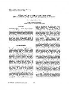
The photodiode spectral distributions are more problematic. As shown in Figure 4, there is considerable overlap between the green and blue photodiode responsivities, even with an external infrared blocking filter. This complicates the analysis of colorimetric measurements, but it is not an insurmountable problem. What is missing from the manufacturer’s data sheet is the expected variance in photodiode spectral responsivities. Without this information, it is difficult to analytically design a reliable architectural dimming control that includes color control for multicolor HBLED-based luminaires.
4. PSYCHOPHYSIOLOGICAL PARAMETERS If an architectural dimming control is to offer the full color gamut of RGB HBLEDs, the user will naturally expect it to provide perceptually linear operation. For example, the control might include dials or sliders for hue, saturation and intensity. Assuming constant saturation and intensity, the hue control should provide linear changes in hue throughout the color gamut. This is an inherently nonlinear control problem. Linear control of the RGB intensities will provide nominally linear movement through the CIE 1931 chromaticity diagram, which is perceptually nonlinear. This nonlinearity can be alleviated but not eliminated by performing a linear transformation to the CIE 1960 L u v color space7. There are other complicating factors. The various CIE color spaces assume that color at a given luminance is linearly additive, but it is not. For example, adding red and white light generally produces a pinkish light whose perceived brightness is less than the sum of the individual lights – they are subadditive. Conversely, violet and white lights are superadditive. We also perceive deeply saturated colors as being brighter than photometric measurements indicate. Red colors can appear up to four times brighter, while violet colors can appear up to nine times brighter6. Another example is that the isocontour lines of constant hue with respect to saturation are nonlinear in any linear color space19. These nonlinearities are fairly subtle in terms of architectural lighting, but they should still be taken into consideration. Finally, the human visual system has a nonlinear response to luminance that is approximately described by Stevens’ power law27: B ∝ L0.5
(2)
where B is perceived brightness and L is luminance. This relationship is commonly incorporated in high-end architectural and theatrical dimmers, where it is referred to as “square law dimming.” Designing a dimming control to take all of these factors into account is a definite challenge. Not only are the psychophysiological parameters nonlinear, some of the basic vision research needed to characterize them is still incomplete.
5. OPERATIONAL PARAMETERS The operational parameters of an architectural dimming control consist of input and output parameters. 5.1
Input Parameters
The obvious input parameters for an architectural dimming control are the spectral radiant intensities as determined by the sensor, and also the approximate luminous intensity. The latter input can be obtained either by appropriately scaling and summing the red, green, and blue sensor inputs or measuring it directly. (The sensor technically measures spectral irradiances and illuminance; relative HBLED intensities are inferred from these measurements.) A previous paper by the author3 suggested that a multicolor HBLED dimming control should allow the user to orthogonally adjust both the correlated color temperature (CCT) and the tint in CIE 1960 L u v color space. To this can be added not only intensity control, but also “daylight harvesting” wherein the sensor monitors the ambient illumination of an interior space and dims the luminaires according to the amount of daylight penetration.
5
The ability to control the color further allows the correlated color temperature of the luminaires to automatically track the daylight chromaticity. This can be done even when there is no significant daylight penetration into the interior space, the advantage being that occupants will have a psychophysiological connection to the outside environment and hourly weather26. Daylighting and human factors research has shown that the optimal design of a daylight harvesting system requires more than simple linear feedback20. While there is still debate over the best approach (and indeed there is unlikely to be a universal solution), it will probably involve a nonlinear transfer function in the feedback loop. 5.2
Output Parameters
The output parameters for an architectural dimming control are the instantaneous drive current values for each color channel. This means at a minimum three channels for red, green, and blue HBLEDs. Future generations of HBLEDbased luminaires may incorporate amber HBLEDs to improve the color rendering indices33; they may also include independent control of individual HBLEDs from different color bins to provide better colorimetric control with varying luminous intensity.
6. DESIGN GOALS The design goals for an architectural dimming control can now be stated in view of the above: • • •
Maintain constant intensity Maintain constant chromaticity Provide fast response to intensity or chromaticity changes with negligible overshoot
The last design goal is particularly important. Above all else, the lighting system (luminaires, sensors and dimming controls) should not be seen to “hunt” for the specified intensity and chromaticity in response to new user setting. At the same time, specifying new intensity and chromaticity values should result in any dimming control producing results that are essentially independent of variations in HBLED and sensor parameters, regardless of the operating conditions. Reviewing the above reveals the most significant HBLED design parameters to be junction temperature, binning (intensity and color), thermal time constants, and nonlinear color space mapping. Similarly, the significant sensor design parameters are per-channel responsivities. (The variances of the spectral responsivities are unknown.) Taken together, these represent operational dependency on a dozen or more variables. The conventional approach to such a problem is to implement a proportional integral-derivative (PID) controller whose feedback control signal is a weighted sum of the instantaneous error, the integral of the error, and the derivative of the error:
∫
m = K c e + K i edt + K d de dt
(3)
where Kc is the instantaneous error (proportional term) weight, Ki is the integral term weight, and Kd is the derivative term weight. These weights are then determined experimentally using the Ziegler-Nichols or a similar feedback loop tuning method32. However, this approach implicitly assumes that the process being controlled is linear. The combination of junction temperature dependencies, square law dimming, and color space mapping may therefore preclude the effective use of linear PID controllers. The simplest approach to controlling nonlinear systems is to linearize the error signal, which can then be used as an input to a PID controller. The problem then becomes one of determining an appropriate nonlinear mapping function.
7. NEURAL NETWORKS Neural networks are known to be universal approximators capable of representing any continuously differentiable bounded function9. While they have not previously been used for architectural dimming or HBLED applications, they have been applied to related problems such as color printer and scanner characterization2, 30, digital image color correction and conversion29, color appearance models4, white point estimation and camera calibration5, 31, color constancy8, and spectrophotometer calibration11.
6
In this paper we use a radial basis function (RBF) neural network to represent the multidimensional function and provide the feedback signals24 needed to maintain constant chromaticity. It is not necessary or even desirable to have an analytic expression for the function. Instead, a neural network can be trained to learn the function with example input data and known or desired output data. The network can therefore be trained on the factory floor using a predetermined set of inputs (i.e., intensity and chromaticity settings) and the desired responses. The neural network implicitly learns the multidimensional function defined by the sensor and HBLED characteristics of each luminaire. This provides a flexible solution that is mostly independent of LED manufacturing tolerances and binning parameters. 7.1
Radial Basis Function Networks
As shown in Figure 5, the RBF network is a feedforward architecture with an input layer, one hidden layer, and an output layer. The input layer has n neurons‡, corresponding to the n elements of the input vector x. The hidden layer has h neurons and one bias neuron, with each input neuron fully connected to the h hidden layer neurons. Each hidden layer neuron (including the bias neuron) is connected to the m output neurons, and has the following activation function§: x − ci i = 1,2, , n exp − y i = 2σ 2 (4) i=0 1 which, apart from the bias neuron, is an n-dimensional Gaussian function with center c and width σ. The expression x − c represents the Euclidean distance from the input vector x to the hidden layer neuron center c in the
K
multidimensional space ℜ n . Each output layer neuron represents one of m possible outputs for the input vector. The output values of these neurons are given by: zj =
h
∑ yi wij i =0
j = 1,2,
K, m
(5)
where wij is the weight between the ith hidden layer neuron and the jth output layer neuron. In operation, an arbitrary input vector x is presented to the RBF network. Each hidden layer neuron computes its output, and the results are presented to the output layer. Each output layer neuron performs a linear weighted summation of the hidden layer neuron outputs. The input vector x is thereby nonlinearly mapped to the output vector z. Considered in terms of an architectural dimming control (Figure 1), an RBF network will have n = 7 input neurons for the sensor inputs and m = 3 output neurons for the HBLED driver outputs. The number of hidden neurons will vary, depending on the complexity of the multidimensional function to be approximated. A generic dimming control design is shown in Figure 1, where the feedback loop consists of the spectral radiant and luminous flux transferred from the HBLEDs to the color sensors. The RBF network linearizes these error signals for presentation to the PID controller.
7.2
Training RBF Networks
Training an RBF network consists of: (1) determining the centers and widths of the hidden layer neuron activation functions; and (2) determining the weights needed for the output layer neurons. There are numerous training strategies, ranging from selecting hidden neuron centers at random from a training set of input vectors13 to applying regularization theory12, 25.
7.2
Center Determination
For center determination, Moody and Darken21 and Musavi et al.22 used k-means clustering to minimize the number of hidden layer nodes needed to approximate the input-output mapping. That is, the training set of input vectors x is ‡
A neural network neuron is a simplified computational model of a biological neuron. It can be thought of as a nonlinear amplifier, typically with a gain of unity or less. § The neuron activation function is equivalent to an amplifier transfer function in that it specifies the output signal in terms of the input signal.
7
clustered in ℜ n by class, with each cluster being assigned to a hidden layer node. More recently, Hwang and Bang10 proposed an efficient one-pass clustering algorithm that they called APC-III. It is more efficient than k-means clustering because it requires only a single pass through the training set. Moreover, it tends to produce an appropriate number of clusters because it determines the radius of a cluster based on the distribution of training vectors.
7.2.2
Width Determination
For width determination, Moody and Darken21 used a simple heuristic that Hwang and Bang10 found worked well in practice. It is: Find the distance to the center of the nearest cluster which belongs to a different class and assign this value multiplied by β to the width. for which Hwang and Bang used β = 0.5.
7.5
Weight Calculation
The weights assigned to the output layer of neurons can be iteratively determined using the Least-Mean-Square (LMS) algorithm (e.g., Haykin9). This algorithm can be expressed as: Input: training vector x Var: d desired response e error η learning parameter w weight vector DO e = d - wTx w = w + ηex WHILE not converged
The rate of convergence for the LMS algorithm can be problematic. Haykin9 offered the heuristic that the number of iterations required is typically ten times the dimensionality of the input space. It is also acutely dependent on the correlation between input vectors in the training set. On the other hand, Luo17 proved that RBF networks will always converge (albeit to a possibly local minimum) when the LMS algorithm is used. There are variations of the LMS algorithm (e.g., Pandya23) that offer faster convergence. However, they are either more prone to local minima convergence or numerically sensitive to the input data. The LMS may be slow to converge, but it is robust and its stochastic nature favors convergence to the global minimum.
8. EXPERIMENTAL RESULTS As of this writing, a hardware implementation of the above architectural dimming control is still under development. In the interim, a mathematical model has been created as a testbed for firmware development and validation. It supports random color and intensity binning, junction temperature dependencies, ambient temperature, thermal resistance, heat capacity, and photodiode spectral responsivities. Preliminary experiments with this model have demonstrated that RBF networks in combination with PID controllers are capable of maintaining perceptually constant intensity and chromaticity under a range of operating conditions. It was decided however that it would be premature to publish these results without physical validation of hardware implementations. An issue worth mentioning is the non-additivity of saturated colored lights that was briefly discussed in Section 4. The luminance of various colors is based on the CIE V(λ) spectral responsivity function7, which was determined by flicker photometry. This technique yields more consistent results than heterochromatic brightness photometry, but it does not adequately describe how we perceive broad expanses of saturated colors. This has important consequences for multicolor HBLED-based luminaires that provide a full color gamut. Surprisingly, this issue has yet to be investigated
8
by the vision research community. This work has necessarily become part of our research program to develop an architectural dimming control, and will be the subject of a future paper.
9.
CONCLUSIONS
This paper describes the rationale, design, and implementation of an architectural dimming control for multicolor HBLED-based luminaires. An in-depth review of the design parameters demonstrates that the control function is necessarily nonlinear, and so a radial basis function (RBF) neural network is proposed to linearize the input to a linear proportional integral-derivative (PID) controller. Unfortunately, the scope of the research has grown steadily and substantially. The research is still in progress, and quantitative results are not yet available for presentation. Nonetheless, the fundamental principles of radial basis functions for feedback control are sound, and we remain confident that they will prove useful for multicolor HBLED dimming control.
REFERENCES 1. 2. 3. 4. 5. 6. 7. 8. 9. 10. 11. 12. 13. 14. 15. 16. 17. 18.
ANSLG. 2001. Specifications for the Chromaticity of Fluorescent Lamps, ANSI C78.376-2001. Rosslyn, VA: American National Standards Lighting Group – National Electrical Manufacturers Association. Artusi, A., and A. Wilkie. 2001. “Color Printer Characterization Using Radial Basis Function Networks,” Color Imaging: Device-Independent Color, Color Hardcopy, and Graphic Arts VI, PIE Vol. 4300, pp. 70–80. Ashdown, I. 2002. “Chromaticity and Color Temperature for Architectural Lighting,” Solid State Lighting II, SPIE Vol. 4776, pp. 51–60. Campadelli, P., C. Gangai, and R. Schettini. 1999. “Learning Color-Appearance Models by Means of FeedForward Neural Networks,” Color Research and Application 24(6):411–421. Cardei, V., B. Funt, and K. Barnard. 1999. “White Point Estimation for Uncalibrated Images,” Proceedings of the IS&T/SID Seventh Color Imaging Conference: Color Science, Systems and Applications, pp. 97–100. Chapanis, A., and R. M. Halsey. 1955. “Luminance of Equally Bright Colors,” Journal of the Optical Society of America 45(1):1–6 (January). CIE. 1986. Colorimetry, 2nd Edition, CIE Publication 15.2-1986. Vienna, Austria: CIE Central Bureau. Funt, B.V., and V. C. Cardei. 1999. “Bootstrapping Color Constancy,” Human Vision and Electronic Imaging IV, SPIE Vol. 3644, pp. 421–428. Haykin, S. 1999. Neural Networks: A Comprehensive Foundation, Second Edition. Upper Saddle River, NJ: Prentice Hall. Hwang, Y.-S., and S.-Y. Bang. 1997. “An Efficient Method to Construct a Radial Basis Function Neural Network Classifier,” Neural Networks 10(8):1495-1503. Lee, H. P., and M. R. Luo. 1998. “Calibrating Spectrophotometers Using Neural Networks,” Color Imaging: Device-Independent Color, Color Hardcopy, and Graphic Arts III, SPIE Vol. 3300, pp. 274–282. Leonardis, A., and H. Bischof. 1998. “An Efficient MDL-Based Construction of RBF Networks,” Neural Networks 11(5):963–973. Lowe, D. 1989. “Adaptive Radial Basis Function Nonlinearities and the Problem of Generalization,” First IEE International Conference on Artificial Neural Networks, pp. 171–175. Lumileds Lighting. 2002. Lumileds Seattle Seminar Notes. October 17, Seattle, WA. Lumileds Lighting. 2002. Luxeon Product Binning and Labelling, Lumileds Technical Datasheet AB21. San Jose, CA: Lumileds Lighting. Lumileds Lighting. 2003. Power Light Source Luxeon Emitter Data Sheet, Lumileds Technical Datasheet DS25. San Jose, CA: Lumileds Lighting. Luo, Z.-Q. 1991. “On the Convergence of the LMS Algorithm with Adaptive Learning Rate for Linear Feedforward Networks,” Neural Computation 2(3):226-245. MacAdam, D. L. 1942. “Visual Sensitivities to Color Differences in Daylight,” Journal of the Optical Society of America 32(5):247–274.
9
19. MacAdam, D. L. 1972. “Perceptually Uniform Spacing of Equiluminous Colors and the Loci of Constant Hue,” Proceedings of the Symposium on Color Metrics, pp. 147–159. (Reprinted in Selected Papers in Colorimetry – Fundamentals, SPIE Milestone Series, Volume MS77, 1993.) 20. Mistrick, R., C.-H. Chen, A. Bierman, and D. Felts. 2000. "A Comparison of Photosensor-Controlled Electronic Dimming In A Small Office." Journal of the Illuminating Engineering Society 29(1):66–80. 21. Moody, J., and C. J. Darken. 1989. “Fast Learning in Networks of Locally-Tuned Processing Units,” Neural Computation 1:281-294. 22. Musavi, M. T., W. Ahmed, K. H. Chan, K. B. Faris, and D. M. Hummels. 1992. “On the Training of Radial Basis Function Classifiers,” Neural Networks 5:595-603. 23. Pandya, A. S., and R. B. Macy. 1996. Pattern Recognition with Neural Networks in C++. Boca Raton, FL: CRC Press. 24. C. Pereira, J. Henriques, and A. Dourado. 1997. “Adaptive RBFNN versus Self-Tuning Controller: An Experimental Comparative Study”, Proceedings of European Control Conference (ECC 97), Brussels, Belgium. 25. Poggio, T., and F. Girosi. 1990. “Networks for Approximation and Learning,” Proceedings of the IEEE 78(9):1481–1497 (September). 26. Rea, M. S., M. G. Figueiro, and J. D. Bullough. 2002. “Circadian Photobiology: An Emerging Framework for Lighting Practice and Research,” Lighting Research & Technology 34(3):177-190. 27. Stevens, J. C., and S. S. Stevens. 1963. “Brightness Function: Effects of Adaptation,” Journal of the Optical Society of America 53:375–385. 28. TAOS. 2003. TCS230 Programmable Color Light-To-Frequency Converter, Data Sheet TAOS046. Plano, TX: Texas Advanced Optoelectronic Solutions Inc. 29. Tominaga, S. 1998. “Color Conversion Using Neural Networks,” Color Imaging: Device-Independent Color, Color Hardcopy, and Graphic Arts III, SPIE Vol. 3300, pp. 66–75. 30. Vrhel, M. J., and H. J. Trussell. 1999. “Color Scanner Calibration via a Neural Network,” Proceedings of IEEE ICASSP ’99, Vol. 6, pp. 3465–3468. 31. Zhou, S., and D. Zhao. 1998. “Neural Network Method for Characterizing Video Cameras,” Electronic Imaging and Multimedia Systems II, SPIE Vol. 3561, pp. 62–68. 32. Ziegler, J. G., and N. B. Nichols. 1942. “Optimum Settings for Automatic Controllers,” Transactions of the ASME 64:759–768. 33. Žukauskas, A., M. S. Shur, and R. Caska. 2002. Introduction to Solid-State Lighting. New York, NY: WileyInterscience.
Intensity Sensor Color Sensors Intensity Control
Radial Basis Function Neural Network
Red HBLEDs PID Controller
HBLED Drivers
Green HBLEDs
Blue HBLEDs Chromaticity Controls
Figure 1 – Generic Dimming Control Design
10
0.9 520 530 0.8
540
510 0.7
550 560
0.6
570
500 0.5
580
y
590
0.4 0.3
600
610 630
490
0.2 480
0.1
470 460
0.0 0.0
0.1
0.2
0.3
0.4
0.5
0.6
0.7
0.8
x Figure 2 – HBLED chromaticity ranges (adapted from Ref. 14)
2.2 2
Relative Light Output
1.8 1.6 1.4
Red
1.2
Green Blue
1
Amber
0.8 0.6 0.4 0.2 0 -20
0
20
40
60
80
100
120
Junction Temperature (Celsius)
Figure 3 – Junction Temperature Dependencies (adapted from Ref. 16)
11
1 0.9
Relative Responsivity
0.8 0.7 Red
0.6
Green
0.5
Blue 0.4
Clear
0.3 0.2 0.1
74 0
70 0
66 0
62 0
58 0
54 0
50 0
46 0
42 0
38 0
34 0
30 0
0
Wavelength (nm) Figure 4 – Photodiode Spectral Responsivity (adapted from Ref. 28)
y0
Bias
y1 x1
z1
x2
zm xn yh
Figure 5 – Radial Basis Function Neural Network Architecture
12