Psychological Review 2010, Vol. 117, No. 4, 1113–1143
© 2010 American Psychological Association 0033-295X/10/$12.00 DOI: 10.1037/a0020311
Neurally Constrained Modeling of Perceptual Decision Making Braden A. Purcell, Richard P. Heitz, Jeremiah Y. Cohen, Jeffrey D. Schall, Gordon D. Logan, and Thomas J. Palmeri Vanderbilt University Stochastic accumulator models account for response time in perceptual decision-making tasks by assuming that perceptual evidence accumulates to a threshold. The present investigation mapped the firing rate of frontal eye field (FEF) visual neurons onto perceptual evidence and the firing rate of FEF movement neurons onto evidence accumulation to test alternative models of how evidence is combined in the accumulation process. The models were evaluated on their ability to predict both response time distributions and movement neuron activity observed in monkeys performing a visual search task. Models that assume gating of perceptual evidence to the accumulating units provide the best account of both behavioral and neural data. These results identify discrete stages of processing with anatomically distinct neural populations and rule out several alternative architectures. The results also illustrate the use of neurophysiological data as a model selection tool and establish a novel framework to bridge computational and neural levels of explanation. Keywords: perceptual decision making, stochastic accumulator models, mental chronometry, frontal eye field
resembles an accumulation to threshold (Hanes & Schall, 1996) sparked a synthesis of mathematical psychology and neurophysiology (Beck et al., 2008; Boucher, Palmeri, Logan, & Schall, 2007; Bundesen, Habekost, & Kyllingsbaek, 2005; Carpenter, Reddi, & Anderson, 2009; Ditterich, 2006b; Mazurek, Roitman, Ditterich, & Shadlen, 2003; Niwa & Ditterich, 2008; Ratcliff, Cherian, & Segraves, 2003; Ratcliff, Hasegawa, Hasegawa, Smith, & Segraves, 2007; Schall, 2004; Wang, 2002; Wong, Huk, Shadlen, & Wang, 2007; Wong & Wang, 2006). This synthesis is powerful because neurophysiology can constrain key assumptions about the representation of perceptual evidence, the mechanisms that accumulate evidence to threshold, and how the two interact. In this article, we describe a modeling approach that assumes a visual-to-motor cascade in which perceptual evidence drives an accumulator that initiates a behavioral response. We make the crucial assumption that the evidence representation and the accumulation of evidence can be identified with the spike discharge rates of distinct populations of neurons. These neural representations can be used to distinguish among alternative models of perceptual decision making. We distinguished models by the quality of their fits to distributions of response times (RTs) and their predictions of neuronal dynamics that accumulate to a threshold to produce a response. A model in which the flow of information to a leaky integrator is gated between perceptual processing and evidence accumulation provides the best account of both behavioral and neural data, while feed-forward inhibition and lateral inhibition are less important parameters.
Mathematical psychology has converged on a general framework to explain the time course of perceptual decisions. Models that assume perceptual information accumulates to a response threshold provide excellent accounts of decision-making behavior (Bogacz, Brown, Moehlis, Holmes, & Cohen, 2006; Nosofsky & Palmeri, 1997; Palmeri, 1997; Ratcliff & Rouder, 1998; Ratcliff & Smith, 2004; Smith & Van Zandt, 2000; Usher & McClelland, 2001). These accumulator models entail at least two distinct processes: (a) A stimulus must be encoded with respect to the current task to represent perceptual evidence, and (b) some mechanism must accumulate that evidence to reach a decision. Models that assume very different decision-making architectures can account for many of the same behavioral phenomena (S. Brown & Heathcote, 2005; S. D. Brown & Heathcote, 2008; Ratcliff & Smith, 2004). Recently, the observation that the pattern of activity of certain neurons
This article was published Online First September 6, 2010. Braden A. Purcell, Richard P. Heitz, Jeremiah Y. Cohen, Jeffrey D. Schall, Gordon D. Logan, and Thomas J. Palmeri, Department of Psychology, Vanderbilt University. This work was supported by the Temporal Dynamics of Learning Center (SBE-0542013), a National Science Foundation (NSF) Science of Learning Center; Robin and Richard Patton through the E. Bronson Ingram Chair in Neuroscience; NSF Grants BCS-0218507, BCS-0446806, and BCS0646588; Air Force Office of Scientific Research Grant FA9550-07-10192; a grant from the James S. McDonnell Foundation; and National Institutes of Health Grants RO1-MH55806, RO1-EY13358, P30EY08126, and P30-HD015052. We thank G. Woodman for sharing code for the neurophysiological analyses and the Vanderbilt Advanced Center for Computing for Research and Education for access to the high-performance computing cluster (http://www.accre.vanderbilt.edu/research). Correspondence concerning this article should be addressed to Thomas J. Palmeri, Department of Psychology, Vanderbilt University, PMB 407817, 2301 Vanderbilt Place, Nashville, TN 37240-7817. E-mail:
[email protected]
Accumulator Models of Decision Processes Evidence accumulation must be preceded by the perceptual encoding of stimuli according to the current task and potential responses to produce the evidence that accumulates. Perceptual encoding takes time, and this delays the start of the accumulation (see Figure 1). Perceptual processing time has traditionally been 1113
PURCELL ET AL.
1114
we review support for the hypothesis that certain neurons in particular brain structures implement the perceptual processing and evidence accumulation proposed by these models.
Neural Basis of Perceptual Decisions
Figure 1.
Stochastic accumulator model illustration.
estimated as a free parameter (e.g., Ratcliff & Smith, 2004). The product of perceptual processing is known as drift rate and is often estimated as a free parameter that is allowed to vary between stimulus conditions and to vary between and within trials (Ratcliff & Rouder, 1998; but see Ashby, 2000; Logan & Gordon, 2001; Nosofsky & Palmeri, 1997; Palmeri, 1997; Palmeri & Tarr, 2008). Many models assume that drift rate is constant over the course of a trial (Ashby, 2000; Nosofsky & Palmeri, 1997; Ratcliff & Rouder, 1998), but other models assume that it varies within a trial (Ditterich, 2006a, 2006b; Heath, 1992; Lamberts, 2000; Smith, 1995, 2000; Smith & Ratcliff, 2009; Smith & Van Zandt, 2000). Systematic variability in RT across stimulus conditions is generally attributed to systematic variability in drift rate. Many models also allow the starting point (baseline) of the accumulation and the threshold to vary across stimulus conditions (S. Brown & Heathcote, 2005; Ratcliff & Rouder, 1998) and propose different sources of intertrial and intratrial variability (e.g., Ratcliff & Smith, 2004). Alternative models propose different mechanisms for how evidence is combined and accumulated to a threshold (reviewed by Bogacz et al., 2006; Smith & Ratcliff, 2004). Independent race models and their discrete analogue independent counter models assume that evidence for each response accumulates independently; the first accumulator to reach threshold determines which response is made (Smith & Van Zandt, 2000; Vickers, 1970). Drift diffusion models (Ratcliff, 1978; Ratcliff & Rouder, 1998) and their discrete analogue random walk models (Laming, 1968; Link & Heath, 1975; Nosofsky & Palmeri, 1997; Palmeri, 1997) assume that perceptual evidence in favor of one response simultaneously counts as evidence against competing responses. Competing accumulator models (Usher & McClelland, 2001) assume that accumulators’ support for alternative responses is mutually inhibitory; as evidence in favor of one response grows, it inhibits alternative responses more strongly in a winner-take-all fashion (Grossberg, 1976b). These alternative models can vary in other respects, such as whether integration of evidence is perfect or leaky. Different accumulator models make many different assumptions about the representation of perceptual evidence and the mechanisms that use it. We asked whether the assumptions that are necessary to account for behavioral data are consistent with neurophysiological data by systematically evaluating major model assumptions within a modeling framework in which both model inputs and outputs are neurally constrained. Our approach is valid if and only if the data are from neurons that instantiate the perceptual processing and evidence accumulation in question, that is, if the linking propositions (Schall, 2004; Teller, 1984) that map model components to brain structures are valid. In the next section,
The past 10 years have witnessed a new focus of research on the neurophysiological basis of decisions about where and when to move the eyes (Glimcher, 2003; Gold & Shadlen, 2007; Schall, 2003; Smith & Ratcliff, 2004). Three major structures have been studied most extensively: the frontal eye field (FEF), the superior colliculus (SC), and the lateral intraparietal area (LIP). These structures are densely interconnected and comprise a diversity of neuron types. We focus on two major subpopulations of neurons, those with tonic responses to visual stimuli and no saccade-related modulation, termed visual neurons, and those with a very weak modulation after stimulus presentation but pronounced growth of discharge rate preceding saccade production, termed movement neurons (also referred to as buildup neurons). Tonic visual neurons are found in FEF, SC, and LIP, while movement neurons are found in FEF and SC, but much less frequently in LIP. FEF and SC receive converging projections from numerous visual cortical areas (see Figure 2; Schall, Morel, King, & Bullier, 1995; Sparks, 1986). FEF and SC movement neurons issue commands to brainstem nuclei to execute saccadic eye movements (Scudder, Kaneko, & Fuchs, 2002; Sparks, 2002). FEF and SC are also connected with brain regions implicated in cognitive control, including medial frontal and dorsolateral prefrontal cortex (Schall & Boucher, 2007; Schall, Morel, et al., 1995; Stanton, Bruce, & Goldberg, 1995) and the basal ganglia (Goldman-Rakic & Porrino, 1985; Hikosaka & Wurtz, 1983). Thus, these areas lie at the
Figure 2. Connectivity between visual cortical areas and the oculomotor system. Middle temporal (MT), visual area V4, visual area TEO, visual area TE, and lateral intraparietal area (LIP) project to the frontal eye field (FEF). LIP and FEF project to the superior colliculus (SC). FEF and SC project to the brainstem saccade generator. Not pictured are connections between prefrontal cortex and FEF, from LIP to SC, and from the substantia nigra pars reticulata of the basal ganglia to SC and to FEF via the mediodorsal nucleus of the thalamus.
NEURALLY CONSTRAINED MODELING OF DECISIONS
junction between perceptual and motor processing and are anatomically situated to influence the decision to move the eyes (Munoz & Schall, 2003). In monkeys performing visual search, tonic visual neurons modulate their activity to select the target (see Figure 3B); this has been observed in FEF (Schall & Hanes, 1993), SC (Basso & Wurtz, 1997; McPeek & Keller, 2002), and LIP (Ipata, Gee, Goldberg, & Bisley, 2006; Thomas & Pare´, 2007). The selection process is independent of movement production (Juan, Shorter-Jacobi, & Schall, 2004; Murthy, Ray, Shorter, Schall, & Thompson, 2009; Murthy, Thompson, & Schall, 2001; Sato & Schall, 2003; Schall, Hanes, Thompson, & King, 1995; Thompson, 2005; Thompson, Bichot, & Schall, 1997; Thompson, Hanes, Bichot, & Schall, 1996). Tonic visual neurons in FEF, SC, and LIP are hypothesized to represent the behavioral relevance of an object in their receptive field (Findlay & Gilchrist, 1998; Goldberg, Bisley, Powell, & Gottlieb, 2006; Thompson & Bichot, 2005). The findings supporting this hypothesis include the observation that the time course and magnitude of selection (the difference in activity when a target vs. a distractor is in a visual neuron’s receptive field) depend on target– distractor similarity (Bichot & Schall, 1999; Sato, Murthy, Thompson, & Schall, 2001; Sato, Watanabe, Thompson, & Schall, 2003), set size (Basso & Wurtz, 1997; Cohen, Heitz, Woodman, & Schall, 2009b), and task contingencies (Sato & Schall, 2003; Thompson, Bichot, & Sato, 2005; Zhou & Thompson, 2009). Movement neurons in FEF and SC initiate a saccade when their spike rate reaches a threshold (see Figure 3C; J. W. Brown, Hanes, Schall, & Stuphorn, 2008; Dorris, Pare´, & Munoz, 1997; Everling & Munoz, 2000; Fecteau & Munoz, 2003; Hanes, Patterson, & Schall, 1998; Hanes & Schall, 1996; Murthy et al., 2009; Pare´ & Hanes, 2003; Ratcliff et al., 2003, 2007; Sparks & Pollack, 1977; Woodman, Kang, Thompson, & Schall, 2008). The time when
1115
movement neuron activity begins increasing and the rate at which it grows to threshold account for random variability in RT (Hanes & Schall, 1996; Thompson & Schall, 2000; Woodman et al., 2008). The time when movement neuron activity begins increasing accounts for changes in RT when the difficulty of a perceptual decision is manipulated (Woodman et al., 2008). This activity has been associated with the dynamics of accumulator models (Boucher et al., 2007; Carpenter, 1999; Carpenter et al., 2009; Carpenter & Williams, 1995; Ratcliff et al., 2003, 2007). However, the neural source of the variability in accumulation time is not identified (but see Bundesen et al., 2005). Visual neurons are often assumed to represent a source of input that drives movement neurons to threshold (Bruce & Goldberg, 1985; Carpenter, Reddi, & Anderson, 2009; Hamker, 2005b; Heinzle, Hepp, & Martin, 2007; Schiller & Koerner, 1971), but this assumption has not been rigorously evaluated. Another line of research has identified a representation of perceptual evidence for a motion direction discrimination task with the activity of neurons in visual area MT (middle temporal; Ditterich, Mazurek, & Shadlen, 2003; Shadlen, Britten, Newsome, & Movshon, 1996) and the evidence accumulation process with the growth of activity in LIP (Roitman & Shadlen, 2002; reviewed by Gold & Shadlen, 2007). The findings that support this claim include the stimulus-dependent growth of activity of LIP neurons (A. K. Churchland, Kiani, & Shadlen, 2008; Roitman & Shadlen, 2002), the effects of MT and LIP microstimulation on performance (Ditterich et al., 2003; Hanks, Ditterich, & Shadlen, 2006; Salzman, Britten, & Newsome, 1990; Salzman, Murasugi, Britten, & Newsome, 1992), and the effects of motion pulse stimuli on behavior and LIP activity (Huk & Shadlen, 2005). Models based on these linking propositions provide a reasonably clear account of performance in terms of neural processes and statistical principles
Figure 3. Saccade visual search task and frontal eye field (FEF) activity during search. Panel A illustrates example stimulus arrays used for color search (top), motion search (middle; arrows indicate direction of motion), and form search (bottom). The color and motion search included a manipulation of target– distractor similarity, with an example of easy on the left and hard on the right. The form search included only one difficulty condition. Right panels show examples of FEF visual (Panel B) and movement (Panel C) neuron activity during visual search. Easy trials are shown in red, hard trials are shown in green. Solid lines are trials in which the target was in the visual neuron’s receptive field or movement neuron’s movement field, and dashed lines are trials in which the target was outside the neurons’ response fields.
PURCELL ET AL.
1116
(Beck et al., 2008; Ditterich, 2006b; Lo & Wang, 2006; Mazurek et al., 2003; Wang, 2002). However, the activity of neurons in MT and other early visual areas is more dependent on stimulus features than task performance (Law & Gold, 2008). Also, LIP does not initiate saccades (Pare´ & Wurtz, 2001; Wurtz, Sommer, Pare´, & Ferraina, 2001). Some additional processing is necessary to initiate the final choice to act. For saccade generation, FEF and SC movement neurons are the most likely candidates. Thus, we propose that a different set of linking propositions is necessary to explain the full duration of the decision process. We explored a range of accumulator models based on two linking propositions: (a) Perceptual evidence is associated with the activity of visual neurons in FEF, and (b) the accumulation of that evidence is associated with the growth of activity to a threshold by movement neurons in FEF. While this model is based on data obtained from FEF, we believe that the signals produced by FEF visual neurons correspond to counterparts in LIP and SC. Other investigators have described the tonic visual neurons in LIP as integrating sensory signals from extrastriate cortex (Gold & Shadlen, 2007). In this study, we focused on the accumulation process occurring in FEF movement neurons that lead to the initiation of the response, and therefore, we consider the visual neurons as the source of perceptual evidence. Similarly, we believe that the signals produced by FEF movement neurons correspond to counterparts in SC.
Overview At the heart of our theory are the linking propositions that perceptual evidence is reflected in the firing rates of FEF visual neurons and the accumulation of evidence is reflected in the firing rates of FEF movement neurons. We used a novel modeling approach to test the validity of these assumptions. Rather than modeling neural inputs to an accumulator, we used observed visual neuron firing rates as the evidence that was accumulated over time. Figures 4 and 5 illustrate the approach. Visual neuron activity was
recorded from the FEF of monkeys performing a visual search task. Neurons with the target in their receptive field drove an accumulator representing a saccade to the target, and neurons with a distractor in their receptive field drove a response to a distractor. The models predicted a saccadic response when an accumulator unit activity reached a fixed threshold. Saccadic RT was the time to reach the threshold plus the brief oculomotor ballistic time. If visual neuron activity is the perceptual evidence, then the model should correctly predict the observed RT distributions. If movement neuron activity is the accumulation of evidence, then the accumulator model dynamics should predict the movement neuron dynamics observed in neurophysiological recordings (e.g., Boucher et al., 2007; Ditterich, 2006b; Ratcliff et al., 2003, 2007). In the next section, we give the details of the experimental and modeling methodology and present the behavioral and neural data to be predicted. Following the methods, we ask whether visual neuron activity is sufficient to predict behavior and, if so, what architectural assumptions for signal transformation are required. Several models provide a good fit, while others can be ruled out because they fail to predict behavior. We then ask whether the same models can predict the dynamics of movement neurons using the same parameters that fit the behavior. The models with conventional parameters of leakage, feed-forward inhibition, and lateral inhibition fail. However, models in which the flow of information from visual neurons to movement neurons is gated provide the best account of behavior and neural data; feed-forward and lateral inhibition are not necessary. We conclude by discussing the implications of these results for theories of decision making and neural function.
Behavioral and Neurophysiological Methods and Results We analyzed behavioral and neurophysiological data from awake behaving monkeys that have been the basis of previous publications (Bichot, Thompson, Rao, & Schall, 2001; Cohen,
Figure 4. Simulation methods. Spike trains were recorded from frontal eye field visual neurons during a saccade search task. Trials were sorted into two populations according to whether the target (top) or distractors (bottom) were within the neuron’s response field. N spike trains were randomly sampled from each population to generate a normalized activation function that served as model input on a given simulated trial.
NEURALLY CONSTRAINED MODELING OF DECISIONS
1117
Figure 5. General model architecture. Two visual units represent activity when a target is in the neuron’s receptive field, vT, and when a distractor is in the neuron’s response field, vD. The activity of the visual units (far left) on a trial is determined from samples of neural activity as shown in Figure 4. Visual neuron activity serves as input to movement units representing a saccade to the target, mT, and distractor, mD. Models were defined by setting parameters equal to zero to eliminate connections shown in dashed grey (see text for details). RT ⫽ response time.
Heitz, et al., 2009b; Cohen et al., 2007; Sato et al., 2001; Schall, Sato, Thompson, Vaughn, & Juan, 2004; Thompson et al., 2005; Woodman et al., 2008). In this section, we describe how the behavioral and neural data were collected and analyzed and summarize the primary observations. Then, we turn to a detailed discussion of the modeling methods and results that are the focus of our new efforts.
Behavioral Training and Testing Methods Five macaque monkeys (Macaca radiata, Macaca mulatta) were trained to perform a visual search task in which reward was contingent upon a single saccade from fixation to a singleton target among a set of distractors. Animals were required to maintain focus on a central fixation point at the start of each trial. After a variable delay (⬃600 ms), the fixation point vanished, and the search array appeared. Monkeys were rewarded if their first saccade was directed to the target. The array consisted of one target and seven distractors randomly located at eight isoeccentric locations equally spaced around the fixation point. During testing, the eccentricity of the array was adjusted depending on the receptive field properties of isolated neurons. The animal had one opportunity to make a saccade to and maintain fixation on the target for reward. Figure 3A illustrates the search arrays. Three sets of stimuli were used: a set in which the target was defined by color (Sato et al., 2001), a set in which the target was defined by direction of motion within a circular aperture of moving dots (Sato et al., 2001), and a set in which the target differed from distractors in shape (Cohen, Heitz, et al., 2009b). The color and motion search tasks included easy and hard conditions determined by target– distractor similarity. For the color search task, the easy condition required a saccade to a green target among red distractors, while the hard condition required a saccade to a green target among yellow-green distractors; on other sessions, monkeys searched for red among green or red among yellow-
red distractors. For the motion search task, the easy condition required a saccade to a target in which 100% of the dots moved to the right among distractors in which 100% of the dots moved to the left. The hard condition required a saccade to a target with only 50%– 60% of the dots moving in a particular direction; on other sessions, the opposite set of dot motion directions for targets and distractors was used. Easy and hard conditions were randomly interleaved within each session. For the form search task, the target was a T among rotated distractor Ls; on other sessions, an opposite set of targets and distractors was used. No target– distractor similarity manipulation was included in the form search for Monkey Q, although it also took place in the context of other manipulations not analyzed here. The difficulty of this task has been established in humans (Duncan & Humphreys, 1989), and animal performance corresponded to performance in the hard condition of the color and motion search tasks (Cohen, Heitz, et al., 2009b), therefore we label these data as another kind of hard search in all figures and tables. Monkey F performed the color search task. Monkeys L and O performed the motion search task. Monkey M performed both color (Mc) and motion (Mm) search during separate recording sessions that are distinguished in the model fits described below. Monkey Q performed form search. Only movement neurons, no visual neurons, were recorded from Monkey O.
Behavioral Results We were primarily interested in the distribution of saccadic RTs for the various search conditions. Each data set was fitted individually; Table 1 summarizes the observed behavior by monkey and task. In addition, we fitted a pooled data set that combined across Data Sets F, L, Mc, and Mm; observed RT quantiles for the individual data sets were averaged using a standard Vincentizing procedure (Ratcliff, 1979). Figure 6 displays the cumulative RT distributions for each animal and for the pooled RT distribution. Analyses of individual monkeys and the pooled data revealed a
PURCELL ET AL.
1118 Table 1 Mean Response Times and Percent Correct Easy search
Hard search
Monkey (task)
Mean RT in ms (SD)
% Correct
Mean RT in ms (SD)
% Correct
F (color) L (motion) Mm (motion) Mc (color) Q (form) Pooled
187 (38.9) 266 (30.1) 228 (32.2) 209 (21.4) — 210 (43.9)
95.8 98.6 88.2 97.1 — 94.4
228 (67.6) 314 (72.9) 271 (67.0) 349 (96.0) 373 (161.7) 274 (87.4)
70.3 94.5 73.3 78.7 85.6 75.7
Note. Dashes indicate that the animal did not perform an easy version of this task. RT ⫽ response time.
significant difference in mean RT for easy versus hard search, all paired t(22) ⬎ 7.79, p ⬍ .05.
Neurophysiological Methods and Analyses Single-unit neurophysiological recordings in the FEF of behaving monkeys were made using procedures that have been described in detail elsewhere (Schall, Hanes, et al., 1995; Thompson et al., 1996). Before being tested on the visual search task, animals performed a memory-guided saccade task to characterize the response properties of the isolated neuron and define it as a visual neuron, movement neuron, or other neuron (Bruce & Goldberg, 1985). Animals were trained to fixate a central point while a peripheral target was flashed in the receptive field for 80 ms. The task required animals to maintain fixation for 400 –1,000 ms after the fixation spot disappeared. For reward, the animal made a saccade to the remembered location of the target after the fixation spot disappeared. Neural activity during a memory-guided saccade task was used to classify neurons. Neurons were classified as visual neurons if their firing rate rapidly increased in response to the presentation of the visual stimulus in their receptive field but showed no increase
in activation prior to a saccade. Neurons were classified as movement neurons if their activity remained at baseline in response to the presentation of the visual stimulus but showed an increase in activation prior to a saccade within their movement field, the area of the visual field to which a saccade is executed when activity reaches threshold. FEF neurons have heterogeneous response properties (Bruce & Goldberg, 1985), and two groups of visually responsive neurons were excluded from our analyses. First, FEF visuomovement neurons that show both visual and movement-related activity were excluded. There is neurophysiological (Murthy et al., 2009; Ray, Pouget, & Schall, 2009) and biophysical (Cohen, Pouget, Heitz, Woodman, & Schall, 2009) evidence that visuomovement neurons are a distinct class of neurons apart from pure visual and movement neurons. The simulations presented in this article are limited to pure visual and pure movement neurons because the distinction between these populations is well established both functionally (Murthy et al., 2009; Thompson, 2005; Thompson et al., 1997) and anatomically (Pouget et al., 2009; Segraves, 1992). We also conducted simulations in which visuomovement neurons were included, and the key model predictions were unchanged. Nevertheless, there is evidence that visuomovement neurons may reflect a corollary discharge to update visual processing (Ray et al., 2009), and so it remains an open question to what degree visuomovement neurons can be functionally grouped with either pure visual or pure movement neurons. Second, FEF phasic visual neurons that show a brief visual response to a stimulus that does not select the location of the target were excluded from our analyses (Bruce & Goldberg, 1985; Thompson et al., 1996). This assumes that the neurons that signal relevant stimuli are the neurons that contribute most strongly to preparation of a response (e.g., Bichot, Thompson, et al., 2001; Ghose & Harrison, 2009; Purushothaman & Bradley, 2005; but see Shadlen et al., 1996). A visual neuron was said to select the target if the area under the receiver-operating characteristic (ROC) curve calculated from trials in which a target was in the neuron’s receptive
Figure 6. Observed behavioral data. Cumulative distribution of correct response times (RTs). RTs from easy trials are red, hard are green. Each panel indicates a different data set. Monkey F (color search), L (motion search), M (Mc ⫽ color, Mm ⫽ motion search), pooled (Vincentized RT distribution from F, L, and M), and Q (form search).
NEURALLY CONSTRAINED MODELING OF DECISIONS
field and trials in which a distractor was in the neuron’s receptive field reached 0.70 prior to the mean saccade RT in either difficulty condition (Thompson et al., 1996). We also explored simulations that included neurons that did not reach 0.70 in ROC area. Larger samples of trials were necessary to signal the location of the target, but major conclusions were unaffected. Inclusion criteria for movement neurons were as follows: All neurons that showed a sharp increase in activity immediately preceding the saccade during the memory-guided search task were included in the movement neuron analyses. We also included a small number of movement neurons that showed a minimal visual response but predominately responded immediately prior to saccade. Movement neurons recorded with less than 30 correct behavioral trials were not included. We also adopted several trial-specific inclusion criteria: (a) Only trials in which a saccade was correctly made to the target were included1; (b) trials in which the animal broke fixation early, failed to maintain fixation on the target, or shifted gaze away from the search array entirely were not included in these simulations (⬍0.7% total trials); (c) trials in which the animal anticipated the target location (RT ⬍ 100 ms) or the animal did not respond within a time window (RT ⬎ 2,000 ms) were excluded from analysis (⬍0.03% of total trials); and (d) trials in which a distractor fell within the neuron’s receptive field but the target appeared in an adjacent location were excluded for two reasons: First, FEF receptive fields are irregularly shaped, and it is difficult to guarantee that the target is completely outside the neuron’s receptive field. Second, a subset of visual neurons exhibits enhanced suppression of stimuli at the border of the receptive field, and the effect of this inhibition will be inconsistent across different neurons (Schall & Hanes, 1993; Schall, Hanes, et al., 1995; Schall et al., 2004).
Neurophysiological Results A total of 64 visual neurons met the inclusion criteria outlined above (11 neurons from F, three from L, six from Mm, four from Mc, and 40 from Q).2 Figure 3B shows the response of a representative visual neuron during easy and hard visual search. Visual neurons typically show an initial indiscriminate response to both target and distractor in their receptive field after a search array appears. However, over time, visual neuron activity evolves to signal the location of the target before a saccade is generated. Across neurons, target selection is achieved by a decrease of the response evoked by distractors and the maintenance or enhancement of the response evoked by a target. Divergence between target and distractor activity is delayed, and the difference is slower to evolve for hard search than for easy search (Bichot & Schall, 1999; Cohen, Heitz, et al., 2009b; Sato et al., 2001). Activity patterns were similar during color, motion, and form search. Of primary interest is whether visual neuron activity is sufficient to be the representation of perceptual evidence that is accumulated by movement neurons. Sixty-one movement neurons met the inclusion criteria described above (34 neurons from F, five from L, five from Mm, four from Mc, three from O, and 10 from Q). Figure 3C shows the activity of a representative movement neuron during the
1119
easy and hard conditions of the visual search task when a saccade was made to the target. The figure illustrates the characteristic buildup of movement neuron activity prior to a saccade to a target. There is often little activity of movement neurons that would signal a saccade to a distractor, although this varies across neurons. When trials are aligned on the time of saccade initiation, activity rises to a constant threshold level immediately prior to the eye movement. This pattern holds across difficulty conditions. Further quantitative analyses of both movement neurons and simulated model accumulators are reported later in this article.
Modeling Methodology A fundamental innovation of our approach was to use the actual spike rate of recorded neurons as the input to alternative accumulator models. For each monkey, visual neuron activity recorded during individual trials of the visual search tasks was divided into two populations (see Figure 4). The first population consisted of trials that were recorded when the target fell in the neuron’s receptive field. The second population consisted of trials that were recorded when a distractor fell in the neuron’s receptive field. For each simulated trial, we randomly sampled, with replacement, N spike trains from the population of trials in which the target fell in a neuron’s receptive field—the input to the accumulator for a decision to saccade to the target location—and N trials from the population of trials in which a distractor fell in a neuron’s receptive field—the input to the accumulator for a decision to saccade
1
The task is relatively simple, and there were very few error trials, particularly in the easy condition. To evaluate the model’s predictions of errors, populations of trials would need to be split into the following two populations: (a) trials in which the target appeared in the neuron’s receptive field but a saccade was made to another distractor and (b) trials in which a distractor appeared in a neuron’s receptive field and a saccade was made to that location. The number of error trials that met these criteria was very low in most of these data sets, making simulations where visual neuron activity drives accumulator models impossible. We should note that FEF visual neurons do select the location of the distractor to which an erroneous saccade is made during saccade search tasks (Cohen, Heitz, Woodman, & Schall, 2009a; Thompson et al., 2005; but see Trageser, Monosov, Zhou, & Thompson, 2008). This is in agreement with the predictions of our framework. 2 Our simulations randomly sampled trials of activity with replacement. Each data set provided a sufficiently large number of trials from which to sample when the target was in the neuron’s receptive field (easy: F, 883; L, 267; Mm, 432; Mc, 177; pooled, 1,759; hard: F, 635; L, 271; Mm, 451; Mc, 195; Q, 5,696; pooled, 1,552) and when a distractor was in the neuron’s receptive field (easy: F, 2,202; L, 501; Mm, 730; Mc, 746; pooled, 4,179; hard: F, 1,586; L, 517; Mm, 778; Mc, 689; Q, 11,724; pooled, 3,570). The complete data sets for L and M were not large, L: 11 neurons total (five visual), Mm: 18 neurons total (seven visual), Mc: 11 neurons total (six visual), but there were no consistent differences between these data sets and other data sets that used a larger population of neurons (F, Q, pooled). One data set, Mc, consistently fit the data worse than other data sets. This may have been due to lower trial numbers.
1120
PURCELL ET AL.
to the distractor location.3 The number of trials sampled from each population was varied systematically from N ⫽ 1 to 24. Fits were not improved by increasing N above this range, which reflects our choice to only sample from visual neurons that select the location of the target (e.g., Bichot, Thompson, et al., 2001).4 We generated an average activation function (spike density function) from the collection of spike train trials by convolving the spikes with a kernel resembling a postsynaptic potential (Thompson et al., 1996). This visual neuron activation function was the input to each accumulator on a simulated trial. Trials from multiple neurons were combined into a single average activation function. The tonic firing rates of FEF neurons are highly variable, therefore we weighted the input from each neuron by the reciprocal of its maximum firing rate. The result was a normalized activation function for visual neuron input for target and distractor with a maximum of 1 and minimum of 0. This computation was necessary so that contributions were not overly weighted by neurons that discharged, on average, at a much higher rate. It is plausible that the brain implements a similar normalization operation (Grossberg, 1976a; Heeger, 1992). Visual neuron activity was recorded throughout the duration of the visual search task. Each simulated trial began 300 ms before the presentation of the visual search array while the animal fixated the center of the screen. The models were active from this point until the saccade decision was made; in other words, input flowed continuously throughout the simulation. Starting simulations at a constant time prior to the appearance of the search array eliminated the need for free parameters that would determine the initial value of the accumulator (the starting point, or baseline), the duration of perceptual processing (predecision time, or the time when the accumulation begins), and any parameters that would govern how those values vary across trials and conditions. Instead, intratrial changes depended entirely on the nonstationary input function derived from the recorded visual neuron activity (see Figures 3B and 4). This also allowed us to explore predicted model dynamics from before the search array onset until the saccade was made, which had important implications for model selection. Visual neurons were classified according to the object in their receptive field, but this classification is meaningful only up until a saccade is made and gaze shifts. This raises the question, What should be done with the firing rates for neurons on trials in which a saccade occurred before the model reached threshold? Simply dropping postsaccade activity inflated variability in the visual signals and caused simulations to terminate without any response, which causes problems for the fit routine where initial parameters may predict very long RTs. Our solution was to extrapolate visual neuron activity beyond the time when a saccade was made when that particular neuron was recorded on a particular trial with a longer RT. The distribution of interspike intervals for cortical neurons is approximately Poisson (Rodieck, Kiang, & Gerstein, 1962), so we generated spike trains according to a homogeneous Poisson process with a rate parameter equal to the mean spike rate in the interval 20 ms to 10 ms prior to a saccade. Essentially, this extended the neuronal spike train at a constant rate. Importantly, for well-fitting models that predicted the observed range of RTs, these extrapolated portions of visual neuron input contributed little to the predicted model activation. On each simulated trial, the model input consisted of two visual activations: vT (t), activation from visual neurons with the targets in
their receptive field, and vD(t), activation from visual neurons with distractors in their receptive field. The visual neuron inputs varied across time and across trials because of the random sampling from recorded neurophysiological trials. Each model consisted of two movement units: mT (t), activation of a movement neuron representing a saccade to the target, and mD(t), activation a model movement neuron representing a saccade to a distractor. RT was
3 In our simulations, we used two accumulators (target vs. distractor) rather than eight (one for each stimulus in the array) or far more than eight (total number of accumulating neurons thought to reside in FEF). Essentially, we have assumed that input driven by each distractor (nonadjacent to the neuron’s receptive field) is pooled into a single unit that races against the target-driven activity. This assumption was necessary for these data sets because increasing the number of accumulators would decrease the populations of trials from which model input could be sampled, and the number of neurons and trials from these previously recorded physiology sessions was already rather limited. In other words, for most of the individual data sets, there were not sufficient trials to simulate a model in this way. The data sets we used all included a fixed set of eight stimuli and always contained a target, so models did not need to predict changes in RT or neural activity with set size. Because the neuron shows maximal activation when the target is in its receptive field, it is unlikely that model predictions would qualitatively change by including multiple competitors. In addition, the vast majority of accumulator model applications have been in the context of two-alternative forced-choice tasks, so this framework also allows us to relate more directly to that broader family of models. To ensure that our conclusions do not depend critically on modeling only two locations, we simulated preliminary versions of the models using an accumulator for multiple locations using the data set, Q, that contained enough trials to sample activity for multiple distractors. The behavioral and neural predictions of the model were qualitatively similar when multiple accumulators were used. 4 How many neurons contribute to a perceptual decision is an open question. The range of the sampled trials used in our simulations is consistent with the findings of other studies examining reliability of neural coding (e.g., Bichot, Thompson, et al., 2001; Ghose & Harrison, 2009). One possible explanation for the small number of sampled neurons is that decisions may be preferentially based on neurons that most reliably signal the relevance of a stimulus (Purushothaman & Bradley, 2005). Even so, these estimates may seem very low relative to the total number of neurons in a given brain region. This may be explained in two ways: First, phasic visual neurons that do not select the target may contribute to the pooled response that ultimately drives movement neurons. We tested models that included sampling from both selective visual neurons and nonselective visual neurons that do not reach 0.70 in ROC area. Not surprisingly, larger samples were needed for the model to reliably select the correct location of the target. Second, the benefits of pooling across many neurons may be limited by correlated noise between neurons (Shadlen et al., 1996). This would put an upper limit on the signal-to-noise ratio of the pooled visual neuron signal, which would be reflected in a relatively low number of sampled trials required in the simulations. While noise correlations between individual FEF visual neurons are relatively weak (⬃0.1; Bichot, Thompson, et al., 2001; Cohen et al., 2010), even small correlations can have profound effects on pooled activity across a large number of neurons (Cohen et al., 2010; Shadlen et al., 1996). Note that for our simulations, the pooled visual activity across our trials was necessarily independent because the neurons were not recorded simultaneously; therefore, we refrain from drawing strong conclusions about the size of the actual neuronal pool based on the present analyses. Future simulations using simultaneously recorded pairs of neurons or simulating spike trains with correlated noise could shed light on this issue.
NEURALLY CONSTRAINED MODELING OF DECISIONS
given by the first movement unit to reach a threshold, . Simulating thousands of trials with different samples of vT (t) and vD(t) led to different trajectories for mT and mD that predicted a distribution of saccade RTs. Several basic assumptions were shared by all models. All parameters were fixed across conditions because easy and hard search arrays were interleaved. All between-condition variability was due solely to observed changes in the visual neuron inputs. Movement unit activation was rectified to be greater than zero because we identified movement unit activity with neuronal firing rate, which cannot be negative. All models compared movement unit activity to a threshold, , whose value was optimized to fit behavior. In the following section, we discuss different models that include additional parameters that determine movement neuron computations. The first movement unit to reach threshold determined whether a saccade was made to the target or distractor. The time when threshold was reached plus a brief ballistic time was the RT. We did not explicitly model activity that followed threshold crossings, but the latency between movement neurons reaching threshold and the generation of a saccade is ⬃15 ms in primates (Scudder et al., 2002). This represents the time necessary for the brainstem mechanisms to initiate a saccadic eye movement. Therefore, the RT predicted for each simulated trial was defined as the time from target onset to the time when threshold was crossed plus a constant ballistic time, tballistic, which was constrained to fall within an interval of 10 –20 ms. We adopted standard model fitting techniques to find values of parameters that provided the best fit to the behavioral data. For a given set of parameter values, we generated 5,000 simulated trials to produce predicted RT distributions for both difficulty conditions. All models were fit to behavioral data using the Simplex routine (Nelder & Mead, 1965) implemented in MATLAB (The MathWorks). We used a Pearson chi-square statistic to quantify the discrepancies between the observed and predicted cumulative correct RT distributions (Ratcliff & Tuerlinckx, 2002; Van Zandt, 2000): 2 ⫽ N
冘
i
共Oi ⫺ Pi兲 2 . Pi
(1)
The summation over i indexes RT bins defined by the quantiles of the observed RT distribution corresponding to the cumulative probabilities of 0.1, 0.3, 0.5, 0.7, and 0.9. Oi are the observed proportion of RTs, Pi are the predicted proportion of RTs within the bins, and N is the total number of data points in the observed RT distribution. With these quantiles, the six Oi are 0.1, 0.2, 0.2, 0.2, 0.2, and 0.1. Pi are the predicted proportion of RTs falling within each bin, which varies with the values of the various parameters. The probabilities are converted to frequencies by multiplying by the observed number of data points, N. The chisquare increases with the difference between the predicted RT distribution and the observed RT distribution. We counted the number of predicted responses falling within the correct RT distribution (Van Zandt, 2000); therefore, the fit routine maximized the proportion of correct responses in addition to matching the distribution of observed RTs. Simplex finds values of free parameters that minimize the chi-square. Five data sets from individual monkeys were fitted separately (F, L, Mc, Mm, and Q), and a pooled data set that
1121
combined across monkeys and stimulus sets was also fitted (F, L, Mm, and Mc). For data sets with an easy and hard condition, both difficulty conditions were fitted simultaneously by summing the individual chi-square statistics for the two conditions. For each model and data set, we ran the Simplex routine using ⬃40 different starting points that were distributed across a reasonable range of parameter space to mitigate the problem of finding local minima during the parameter search. This was done in parallel on the high-performance computing cluster supported by the Vanderbilt Advanced Center for Computing for Research and Education. With only two RT distributions, one for easy search and one for hard search, it did not seem sensible to engage in extensive quantitative tests of model fits. Our goal was instead to find models that provided an acceptable fit to behavior that would later be compared to neural data. To quantify an acceptable fit, we computed a standard R2 fit statistic from the observed and predicted RT percentiles: R2 ⫽ 1 ⫺ (SSerror/SStotal). SSerror was given by squaring the deviation between the observed and predicted percentiles. SStotal was given by squaring the deviations between the observed percentiles and the mean across difficulty conditions. We used a simple heuristic of R2 ⱖ 90% as an acceptable account of behavior. We also included a fit statistic, X2, in which observed proportions were multiplied by 100 rather than the number of observations, thus they were not true frequencies (Ratcliff & Smith, 2004). This statistic facilitated comparisons of fit across data sets because the number of observations varied across individuals. Although we emphasize the use of neural data for model selection, we also compared models on their account of behavior. Standard hierarchical model testing proved problematic for several reasons when running these simulations,5 so we developed an alternative benchmark for when a difference in X2 values was deemed to be too large. To do this, we used the best fitting parameters for a given model to simulate 5,000 RT distributions (each containing 5,000 simulated RTs) that only differed in the initial random number seed. An X2 statistic was computed for each simulation. We then calculated a distribution of differences in X2 values between runs differing only in the randomly sampled inputs. We compared the difference in fit between two tested models 2 2 2 (Xdiff ⫽ XModel 1 ⫺ XModel 2) to these distributions to compute a p value, and the 95th percentile of the distribution was used as an 5 First, these tests are limited to nested models, yet many of the model comparisons we wished to make are between models that are not nested and that have the same number of free parameters. Second, the power of these tests increases with sample size, so one may attain significance simply by running a large number of simulated trials (Busemeyer & Diederich, 2010). Finally, even with 5,000 simulated trials per condition, the difference between two runs of a model using the exact same parameter values but differing in the random number seed at the start of a run produces chi-square differences that can well exceeded the critical chisquare value for nested models differing in one parameter. We considered both parametric bootstrapping (Wagenmakers, Ratcliff, Gomez, & Iverson, 2004) and increasing the number of simulated trials in each model by an order of magnitude. However, these approaches were not feasible given the computational demands of Monte Carlo simulations. Ultimately, our emphasis is on neural predictions made by models with an acceptable behavioral fit, not on detailed quantitative contrasts of the behavioral fits themselves.
PURCELL ET AL.
1122
2 adjusted critical chi-square (Xcrit ); calculations using the true chisquare were qualitatively identical. This gave us a conservative X2 difference that we might expect from chance if the data were produced by the same model that differed only in random factors. Clearly, this approach does not have the statistical rigor of something like parametric bootstrapping, which would require competing models to be fitted 5,000 times. However, that approach was intractable with our current hardware.
Accounting for Response Times Given the tight constraints imposed on the models, the first question to answer is whether RT distributions can be predicted from the responses of FEF visual neurons. If so, then what computations are necessary and sufficient? To address these questions, we fit several stochastic models to the RT distributions observed during the saccade visual search task. We selected models to evaluate assumptions about the mechanisms thought necessary to predict behavior.
Nonintegrated Models The most fundamental assumption of the accumulator model framework is that evidence must be integrated over time. The first models we evaluated assume that moment-to-moment fluctuations in current perceptual evidence are sufficient to trigger the response threshold without any integration over time. Thus, we tested whether a simple nonintegrated race model was sufficient to account for observed behavior: mT 共t兲 ⫽ vT 共t兲.
(2)
mD共t兲 ⫽ vD共t兲.
(3)
difference must be accumulated for a threshold to be crossed when input is stationary. Here, this is not the case. We evaluated how well both nonintegrated models fit the individual and pooled behavioral data. Fits to behavioral data are illustrated in two ways (see Figure 7): First, we presented the predicted cumulative RT distributions for each condition using the pooled data set along with the observed RT quantiles. A model that fits this data set well will predict a cumulative RT distribution that intersects the observed RT quantiles that were fit. Second, we presented a scatterplot of the observed versus predicted quantiles for the data sets from individual monkeys. A model that fits all data sets well will produce a scatterplot distributed near the diagonal. The fit statistics for every data set and model are summarized in Table 2. Figure 7A illustrates the fits of the nonintegrated race model. The predicted cumulative RT distribution indicates a very poor fit to the pooled data set (R2 ⬍ 0). Recall that our null model (SStotal) was given by the mean across conditions, so a negative R2 indicates that these models actually fit worse than a model that simply predicts the mean across conditions. This is due to extreme misses in the upper tails. The fit is similarly poor across individual data sets. The model cannot account for more than 90% of the variance for a single data set (all R2 ⬍ 0.90). Thus, the nonintegrated race model cannot fit the data. The overall fit of the nonintegrated difference model to the pooled data set is also very poor (see Figure 7B; R2 ⬍ 0). The models generally predicted the correct ordering of the difficulty conditions, but the model severely overpredicted the upper tail of the distribution for most data sets. The quality of fit varied for individual data sets but was generally poor. Although the model provided an adequate fit to two data sets (F and Q: R2 ⬎ 0.90), it
Here, movement unit activation is just the current input from the visual neurons. The time at which m(t) reaches threshold varies because the trial-to-trial input v(t) varies. Effectively, activation at time t integrates across relevant visual neurons, but the movement neurons do not integrate across time. One interpretation of this model is that movement neurons simply pool the input from visual neurons at a given point in time and determine when that pooled activity reaches a threshold. We also tested a model that assumes competition between visual neuron inputs but no integration performed by movement neurons. The activity of visual neurons in FEF showed a distinct pattern in which the difference in activity between neurons representing the target and distractors increased gradually over time, as expected for a decision variable (see Figure 3B). The nonintegrated difference model assumes that the difference in visual unit activation between target and distractor is directly compared to a response threshold: mT 共t兲 ⫽ vT 共t兲 ⫺ vD共t兲.
(4)
mD共t兲 ⫽ vD共t兲 ⫺ vT 共t兲.
(5)
Thus, the movement neurons represent the relative support for one response above and beyond the competing response. This is a basic assumption made by some models of LIP (Ditterich, 2006b; Gold & Shadlen, 2007; Mazurek et al., 2003), but in those cases, the
Figure 7. Behavioral predictions of the nonintegrated models. Panel A shows the fits of the nonintegrated race model. Panel B shows the fits of the nonintegrated difference model. Left panels show the predicted cumulative response time (RT) distributions for the pooled data set (solid lines) with observed 10th, 30th, 50th, 70th, and 90th percentiles (open circles). Easy is red, hard is green. Right panels show scatterplots of observed versus predicted quantiles for individual data sets for easy and hard, Monkey F ⫽ E, L ⫽ ⫹, Mm ⫽ ⌬, Mc ⫽ x, and Q ⫽ ●.
NEURALLY CONSTRAINED MODELING OF DECISIONS
1123
Table 2 Best Fitting Model Parameters for All Models and Data Sets Data set
tballistic
N

k
g
2
X2
2 Xcrit
R2
Nonintegrated models Nonintegrated race F L Mm Mc Mcⴱ Q Pooled Nonintegrated difference F L Mm Mc Mcⴱ Q Pooled
0.91 1.27 0.86 0.89 0.84/0.91 0.88 0.94
14.99 14.98 14.99 14.99 15.00 15.00 14.99
16 2 18 13 17 23 13
— — — — — — —
— — — — — — —
— — — — — — —
749.07 7,761.49a 1,451.14 968.60 668.15 7,426.93 8,390.70
21.68 607.21 94.45 87.91 64.59 34.93 119.97
3.12 50.84 9.41 8.15 7.12 5.04 10.82
⬍0 ⬍0 ⬍0 0.46 0.86 0.65 ⬍0
0.51 1.38 0.55 0.62 0.58/0.64 0.53 0.59
15.00 14.98 15.00 15.00 15.00 15.00 15.00
15 1 15 8 8 23 23
— — — — — — —
— — — — — — —
— — — — — — —
528.91 4,032.35a 515.86 318.06 247.60 1,192.19 2,368.56
16.24 377.28 35.23 29.80 23.45 3.19 32.03
2.98 34.53 4.43 3.59 3.35 1.26 4.46
0.94 ⬍0 ⬍0 0.86 0.96 0.98 ⬍0
Perfect integrator models Perfect race F L Mm Mc Mcⴱ Q Pooled Perfect diffusion F L Mm Mc Mcⴱ Q Pooled Perfect competitive F L Mm Mc Mcⴱ Q Pooled
138.26 143.69 179.74 138.10 121.64/200.84 264.97 163.41
15.00 16.85 16.18 13.41 10.00 14.98 14.97
8 4 7 1 1 5 5
— — — — — — —
— — — — — — —
— — — — — — —
2,077.78a 83.39 639.29a 10,178.87a 970.39a 4,528.94a 4,462.08a
29.66 8.62 27.90 253.57 36.10 7.42 41.11
4.81 1.80 3.96 29.15 4.81 2.02 5.53
0.74 0.90 0.71 0.18 0.91 0.89 0.69
27.05 79.05 36.65 48.06 37.38/63.78 64.23 43.04
10.00 15.78 15.88 10.00 13.93 14.93 15.01
15 5 14 4 4 12 10
— — — — — — —
— — — — — — —
— — — — — — —
1,495.25a 27.06 283.41 933.64 322.98 2,775.81 936.29
22.55 2.32 15.70 70.16 27.21 10.51 8.97
3.93 0.88 2.67 7.01 3.69 2.28 1.99
0.17 0.97 0.73 0.71 0.95 0.80 0.87
98.64 119.55 120.89 92.42 81.28/122.82 176.58 105.39
14.95 15.00 14.97 15.00 15.01 15.00 15.03
10 11 23 15 8 19 21
0.0025 0.0034 0.0028 0.0063 0.0039 0.0023 0.0037
— — — — — — —
— — — — — — —
1,699.13 10.39 354.44 1,206.93 380.10 1,119.75 1,922.71
20.98 0.90 24.38 102.74 29.97 2.42 23.55
3.47 0.53 3.64 9.06 3.66 1.05 3.46
0.66 0.98 0.74 0.46 0.92 0.94 0.78
Leaky models Leaky race F L Mm Mc Mcⴱ Q Pooled Leaky diffusion F L Mm Mc Mcⴱ Q Pooled Leaky competitive F L Mm
33.13 100.25 52.72 10.66 27.76/31.53 65.61 49.67
15.00 14.99 14.99 15.00 15.00 15.00 14.99
7 5 10 12 8 20 11
— — — — — — —
0.0178 0.0036 0.0114 0.0753 0.0247 0.0097 0.0124
— — — — — — —
222.10 42.89 143.79 823.83 324.37 134.45 418.04
5.33 5.22 5.31 79.06 30.67 1.70 9.27
1.67 1.42 1.32 7.14 4.21 0.95 2.02
0.98 0.86 0.90 0.51 0.95 0.98 0.94
10.27 69.33 22.04 7.03 9.82/11.82 12.88 23.22
14.98 15.82 15.33 15.03 15.00 15.00 14.95
10 5 8 7 6 15 10
— — — — — — —
0.0210 0.0018 0.0096 0.0667 0.0402 0.0276 0.0111
— — — — — — —
420.61 21.07 253.00 490.18 190.50 713.87 112.62
12.01 2.51 5.72 26.89 17.64 2.50 1.61
2.67 0.99 1.71 3.25 3.01 1.02 0.82
0.88 0.98 0.99 0.88 0.97 0.94 0.99
15.07 118.84 59.12
15.00 15.00 15.00
17 12 9
0.0474 0.0036 0.0001
0.0400 0.0000 0.0096
— — —
171.04 10.28 59.38
6.09 0.82 5.67
1.72 0.97 0.49 0.99 1.44 0.91 (table continues)
PURCELL ET AL.
1124 Table 2 (continued) Data set
Mc Mcⴱ Q Pooled
tballistic
N

22.63 47.31/57.59 65.65 28.91
15.01 15.00 15.00 15.00
Leaky models (continued) 24 0.0517 0.0296 5 0.0005 0.0117 20 0.0000 0.0097 12 0.0151 0.0211
k
2
g
— — — —
X2
2 Xcrit
R2
365.16 218.22 133.94 102.00
33.11 20.57 1.10 1.56
3.49 3.22 0.68 0.77
0.81 0.97 0.99 0.99
Gated models Gated race F L Mm Mc Mcⴱ Mcⴱⴱ Q Pooled Gated diffusion F L Mm Mc Mcⴱ Mcⴱⴱ Q Pooled Gated competitive F L Mm Mc Mcⴱ Mcⴱⴱ Q Pooled
11.66 56.14 11.63 12.32 36.90/54.26 48.22 21.59 17.18
15.00 15.00 15.00 15.00 14.99 15.00 15.00 15.03
9 7 24 8 5 5 19 22
— — — — — — — —
0.0126 0.0000 0.0083 0.0242 0.0067 0.0037 0.0002 0.0003
0.4616 0.3767 0.5435 0.4385 0.2527 0.2225/0.4125 0.5850 0.5782
317.63 53.48 100.23 1,127.52 342.98 195.00 272.78 190.94
6.87 4.13 8.00 76.47 23.85 15.02 2.61 2.33
1.92 1.52 2.26 8.38 3.85 2.78 1.13 1.17
0.98 0.96 0.98 0.61 0.97 0.99 0.99 0.99
7.04 57.25 9.36 3.19 7.65/11.78 10.53 15.28 16.72
14.99 14.85 14.99 15.00 15.00 14.99 14.99 14.99
11 4 10 8 6 15 13 11
— — — — — — — —
0.0172 0.0000 0.0024 0.0308 0.0229 0.0001 0.0050 0.0037
0.1335 0.1524 0.2600 0.3612 0.1496 0.2117/0.3772 0.2000 0.18
488.20 51.21 84.80 486.18 279.16 211.29 365.39 146.64
13.78 2.10 10.49 28.95 20.92 10.74 2.42 1.58
3.05 0.91 2.63 3.60 3.15 3.30 1.07 0.90
0.98 0.97 0.89 0.91 0.97 0.98 0.99 0.99
11.31 58.22 12.39 10.29 44.95/61.04 52.16 21.20 16.81
15.00 15.00 15.00 15.01 14.98 15.01 15.00 14.99
9 6 18 11 5 5 19 20
0.0077 0.0036 0.0136 0.0012 0.0000 0.0000 0.0016 0.0000
0.0088 0.0000 0.0053 0.0388 0.0075 0.0050 0.0001 0.0007
0.4748 0.3409 0.5449 0.3748 0.1566 0.2383/0.4238 0.5850 0.5768
302.49 52.57 84.82 591.52 335.65 192.83 246.14 149.88
6.75 3.44 5.66 75.48 21.41 15.71 2.84 2.35
2.02 1.36 1.81 8.06 3.46 3.52 1.24 1.11
0.97 0.99 0.92 0.53 0.95 0.98 0.99 0.98
Note. 2 indicates the goodness of fit between predicted and observed response time (RT) and distributions on the easy (if performed) and hard search 2 tasks. X2 indicates the same goodness of fit but is not dependent on the number of observations to facilitate comparison across datasets. Xcrit indicates the maximum difference in fit that would be expected by chance. R2 indicates the proportion of variance in RT accounted for by the models. All models 2 ⴱ predicted ⱖ 90% accuracy for every data set except those with values noted with a subscript a (a). Mc indicates a version of the model in which the threshold, , was free to vary between conditions. Mcⴱⴱ indicates a version of the model in which the gate parameter, g, was free to vary between conditions. Dashes indicate that a parameter was fixed to zero for this model.
failed to fit the remaining individual data sets (L, Mm, and Mc: R2 ⬍ 0.86). We conclude that the nonintegrated difference model cannot fit the behavioral data.
Discussion Visual neurons in FEF are hypothesized to combine feature information from early visual areas to represent the visual salience of objects (e.g., Carpenter et al., 2009; Hamker, 2005a; Thompson & Bichot, 2005); therefore, it was possible that temporal integration is unnecessary. The nonintegrated models assume that a response is initiated when the perceptual evidence given by FEF visual neuron activity crosses some threshold. In other words, this hypothesizes that movement neurons simply pool visual neuron inputs and compare that pooled activity level directly to a response threshold but do not integrate that activity over time. However, these models failed to account for behavior regardless of whether the absolute level of activity or a difference in activity was compared to threshold. Some additional mechanism is required to account for behavior. Previous modeling studies strongly suggest temporal integration.
Perfect Integrator Models We next evaluated three models that assume perfect integration of visual neuron inputs. Formally, we characterized each of these perfect integrator models with specific parameterizations of the following equations, dmT 共t兲 ⫽
dt 关v 共t兲 ⫺ u 䡠 vD共t兲 ⫺  䡠 mD共t兲兴 ⫹ T
dmD共t兲 ⫽
dt 关v 共t兲 ⫺ u 䡠 vT 共t兲 ⫺  䡠 mT 共t兲兴 ⫹ D
冑 冑
dt , T
(6)
dt , D
(7)
that specify the change in activation of the movement unit representing a decision to move the eyes to a target (mT) or a distractor (mD) at each time step, dt (dt/ was set to 1 ms in all simulations). Movement units perfectly integrated visual activity (vT and vD) with respect to time and initiated a saccade when activation reached the threshold, , after the ballistic time, tballistic. Inhibitory interactions among response alternatives could be implemented at two levels: (a) Competition between visual neuron
NEURALLY CONSTRAINED MODELING OF DECISIONS
inputs that were determined by the parameter u correspond to feed-forward inhibition (e.g., Hamker, 2005b) or (b) competition between movement units that were determined by a parameter  correspond to lateral inhibition (e.g., Usher & McClelland, 2001). We evaluated a perfect race model (u ⫽  ⫽ 0), in which each unit independently accumulates the activity of a visual neuron representing the object in its receptive field; this corresponds to previous models of two-alternative forced-choice tasks (Smith & Van Zandt, 2000; Vickers, 1970). We evaluated a perfect diffusion model (u ⫽ 1,  ⫽ 0), in which evidence for one response is simultaneously counted as evidence against the competing response; this is a neurally plausible implementation of a onedimensional diffusion process. As a result, movement units integrate the difference between visual neuron inputs (similar to the difference operation proposed by Ditterich, 2006a; Mazurek et al., 2003). Finally, we evaluated a perfect competitive model (u ⫽ 0,  free to vary), in which lateral inhibition between response units at a given time point depends on the current activation of that unit weighted by ; this corresponds to models that implement winnertake-all dynamics through mutually inhibitory units (similar to Usher & McClelland, 2001; see also Wang, 2002, for a detailed neurophysiological implementation). We included a Gaussian noise term, , for both accumulating units with a mean of zero and a standard deviation of . In most implementations of stochastic accumulator models, the only intratrial variability comes from this noise term. However, in our case, there was substantial noise inherent in the input, vT and vD, because input was derived directly from spike trains that are inherently noisy. Thus, we parsed noise into two components: exogenous noise that is inherent in the visual neuron input and endogenous noise that is
1125
intrinsic to the movement units given by . We explored versions of these models with various levels of endogenous noise, but adding noise did not strongly affect most predictions. Therefore, for these models, we assumed that all noise was due to the visual neuron input by fixing ⫽ 0 in all cases. We explore models with endogenous noise later in this article. The fits of the perfect integrator models to the RT distributions are shown in the left panels of Figure 8, and details are given in Table 2. By our criterion, the overall fit was very poor for the race and competitive models (race R2 ⫽ 0.69, competitive R2 ⫽ 0.78) because they severely underestimated between-condition variability. The diffusion model provided a slightly better account of the pooled data set than the race and competitive models (R2 ⫽ 0.87) but still underestimated between-condition variability and missed the upper tail of the hard RT distribution. All models failed to meet our benchmark of accounting for 90% of the variance. The fits to the individual data sets were also poor for each of the perfect integrator models (see Figure 9, left panels). The poor fit can be summarized in the low average R2 (R2 ) across data sets (race R2 ⫽ 0.69, diffusion R2 ⫽ 0.71, competitive R2 ⫽ 0.76). In general, the model fits the data sets of individual monkeys poorly, although there is some variability across data sets.
Discussion Integration appears to be necessary, but models assuming perfect integration could not predict the observed behavior. Why did these models fail when similar models have been successful in accounting for richer sets of data? The models failed because, in our approach, visual neuron activity is input to accumulator units
Figure 8. Behavioral predictions of the perfect (left panels), leaky (middle panels), and gated (right panels) accumulator models to the pooled data set. Each panel shows the predicted cumulative response time (RT) distributions for the pooled data set (solid lines) with observed 10th, 30th, 50th, 70th, and 90th percentiles (open circles). Easy is red, hard is green.
PURCELL ET AL.
1126
Figure 9. Behavioral predictions of the perfect (left panels), leaky (middle panels), and gated (right panels) accumulator models to all data sets. Each panel shows a scatterplot of the observed versus predicted response time (RT) quantiles that were fit by the data. Easy is red, hard is green. Monkey F ⫽ E, L ⫽ ⫹, Mm ⫽ ⌬, Mc ⫽ x, and Q ⫽ ●.
continuously over time. There is no mechanism to limit the rate of accumulation prior to the onset of the stimulus array. Visual neurons do not discriminate the target until late in the trial, which means that units accumulate noise for the majority of the trial. Stimulus-dependent differences in the model inputs have little time to impact the accumulation. Some mechanism is necessary to limit the rate of accumulation until a decision is made. Several plausible mechanisms could be implemented to limit the rate of input to the accumulator units. Many accumulator models circumvent this problem by assuming that the start of the accumulation is delayed relative to the onset of the stimulus. It is plausible that some external signal initiates the accumulation sometime after the stimulus onset. However, a more complete and parsimonious explanation is that some mechanism limits the rate of flow from visual to movement neuron activity until a relevant signal is present. In the following sections, we evaluate two simple mechanisms that perform that function.
Leaky Accumulator Models We first asked whether leaky integration could improve model performance. Leakage in these models is implemented as selfinhibition of a unit that scales with the activation of the unit at a given point in time. We considered leaky versions of the race model, diffusion model, and competitive model as follows: dmT 共t兲 ⫽
dt 关v 共t兲 ⫺ u 䡠 vD共t兲 ⫺  䡠 mD共t兲 ⫺ k 䡠 mT 共t兲兴 ⫹ T
冑
dt , T (8)
dmD共t兲 ⫽
dt 关v 共t兲 ⫺ u 䡠 vT 共t兲 ⫺  䡠 mT 共t兲 ⫺ k 䡠 mT 共t兲兴 ⫹ D
冑
dt . D (9)
Here, k is the leakage constant, and all other variable are as described earlier. Leakage is inherently inhibitory, so k is constrained to be greater than zero. As with the perfect integrator models, we evaluated a leaky race model (u ⫽  ⫽ 0), a leaky diffusion model (u ⫽ 1,  ⫽ 0), and a leaky competitive model (u ⫽ 0,  free to vary). We report values where leakage was optimized to fit behavior, and we also explored the effect of varying the value of the leakage constant incrementally while finding best fitting values of the other parameters. As before, we found that adding small amounts of endogenous noise did not affect model predictions, so it was fixed to zero ( ⫽ 0). The fits of the leaky models to the pooled data set are shown in Figure 8 (center panels). In contrast to the perfect integrator models, all leaky integrator models provided a good account of the pooled data set (all R2 ⬎ 0.90). This improvement in fit, relative to perfect integrator counterparts, was significant for all three 2 models (all Xdiff ⱖ 7.36, all p ⬍ .05). The leaky models also fit nearly all individual data sets very well (see Figure 9; all R2 ⬎ 0.90, except Mc). In general, the fit of the leaky integrator model was significantly better than that of the perfect integrator models. For the race model, the improvement in fit was significant for all 2 data sets (all Xdiff ⱖ 3.38, all p ⬍ .05); for the diffusion model, the improvement was significant for most (four out of five) individual 2 2 data sets (all Xdiff ⱖ 2.27, all p ⬍ .05, except L, Xdiff ⫽ 0.19, p ⫽ .72); and for the competitive model, this improvement was signif-
NEURALLY CONSTRAINED MODELING OF DECISIONS 2 icant for most (four out of five) individual data sets (all Xdiff ⱖ 2 1.32, all p ⬍ .05, except L, Xdiff ⫽ 0.08, p ⫽ .88). Across models, only the Mc data set was fit poorly, which we attribute to low trial numbers. To summarize, the leaky integrator models fit the pooled data and nearly all data sets very well, and the improvement over the perfect integrator models was nearly always significant. We also compared behavioral fits between the leaky race, leaky diffusion, and leaky competitive models, but differences in fit across these models were not consistent enough to draw strong conclusions about the nature of interactions among response units. Leaky integrator models that assume different forms of competition seem able to predict behavior equally well, at least for the behavioral data set we tested.
1127
activity of the movement units. Formally, the following equations defined the gated models: dmT 共t兲 ⫽ dt 关共v 共t兲 ⫺ u 䡠 vD共t兲 ⫺ g兲 ⫹ ⫺ k 䡠 mT 共t兲 ⫺  䡠 mD共t兲兴 ⫹ T
冑
dt , T (10)
dmD共t兲 ⫽ dt 关共v 共t兲 ⫺ u 䡠 vT 共t兲 ⫺ g兲 ⫹ ⫺ k 䡠 mD 共t兲 ⫺  䡠 mT 共t兲兴 ⫹ D
冑
dt . D (11)
Discussion Unlike perfect integrators, models that assume leaky integration predicted the observed behavior. Here, leakage is advantageous because it asymptotically limits the accumulation of perceptual evidence prior to a decision. Visual neuron inputs are approximately constant in the absence of a stimulus, so accumulator activity reaches a lower asymptote when the rate of decay is approximately equal to the input. Following the presentation of the search array, visual neuron inputs increase, so the accumulators begin to increase again until an upper asymptote is reached. If the threshold is placed between the lower and upper asymptotes, then the model will predict a baseline firing rate that increases to threshold when the visual neuron inputs increase. In other words, the leak is constant throughout the trial, but it is the level of input that changes. Thus, leakage provides one way to limit the rate of accumulation in the presence of dynamic neural inputs. Leakage limits the rate at which evidence is accumulated, but evidence still flows continuously to accumulator units. These models assume that visual neurons represent relevant perceptual evidence while movement neurons simultaneously accumulate that evidence over time. Alternatively, a pure discrete stage model would assume that the accumulation of evidence does not begin until perceptual processing is complete, when a representation of perceptual evidence is achieved. This assumption is made by models in which the drift rate is constant and the accumulation begins some delay following the presentation of the stimulus. However, this assumption seems at odds with our neurally constrained framework in which perceptual evidence is defined by a neural representation that evolves continuously over time. In the following section, we evaluate a new set of models assuming that the start of the accumulation is not determined by a fixed delay from the stimulus onset but, like leakage, depends on the level of visual input flowing into the accumulator. In contrast to leakage, input is gated prior to reaching the accumulator until it exceeds a particular level. In this way, these simple models represent a neurally plausible implementation of discrete stages.
Gated Accumulator Models We tested gated models of perceptual decision making that assume dynamic visual neuron input exactly like the continuous flow models described so far but where a gate parameter controls the minimum level of visual neuron input needed to modulate
The gate parameter, g, is a constant inhibition applied to the visual neuron input that drives the accumulators. Mathematically, this is equivalent to constraining the total input to be greater than g for accumulation to begin. Once g is exceeded, it continues to be subtracted from the visual inputs but does not scale with the level of the accumulation. The term (vT (t) ⫺ u 䡠 vD(t) ⫺ g) is constrained to be ⱖ 0 because the gate is applied to the input, not the movement units themselves. In all fits, g was a free parameter that was constrained to be greater than zero. We evaluated a gated race model (u ⫽  ⫽ 0), a gated diffusion model (u ⫽ 1,  ⫽ 0), and a gated competitive model (u ⫽ 0,  free to vary).6 Like the earlier models, we have a term for intrinsic Gaussian noise with a mean of zero and standard deviation, . As before, we found that including noise did not impact behavioral predictions. However, if m(t) starts at zero and g is high enough to suppress input to zero, then there is nothing to accumulate, so the models predicted little to no baseline activation. Most FEF movement neurons have a small tonic baseline firing rate (Bruce & Goldberg, 1985; Schall, 1991; Segraves & Goldberg, 1987); therefore, we included an endogenous noise term to represent stochastic elements in movement neuron activity or the neural circuit. Low levels of intrinsic noise ( ⫽ 0.2) accumulate in movement units, and low levels of leakage cause activation to asymptote at a relatively invariable baseline that is well below threshold. This means that the baseline level of activity is primarily due to intrinsic noise but that the rise of activation to threshold is primarily due to modulations in the visual neuron inputs. The fits of the gated models to the pooled behavioral data are shown in Figure 8. All three gated models provided an excellent account of the pooled data set (race R2 ⫽ 0.99, diffusion R2 ⫽ 0.99, competitive R2 ⫽ 0.98). Compared to their leaky counterparts, only the gated race model fit significantly better than 2 its leaky counterpart (race Xdiff ⫽ 6.94, p ⬍ .05), whereas the fit was not significantly different for the other models (diffusion 2 2 Xdiff ⫽ 0.02, p ⫽ .96; competitive Xdiff ⫽ 0.81, p ⫽ .16). On average, all three gated models accounted for the individual data sets very well (see Figure 9; race R2 ⫽ 0.92, diffusion R2 ⫽ 0.95, competitive R2 ⫽ 0.90), with the exception of Mc. The change in fit between the leaky race and gated race models 6 Working simulations of the accumulator models described in this article can be downloaded from http://catlab.psy.vanderbilt.edu/wpcontent/uploads/PurcellHeitzCohenLoganSchallPalmeri_PublicCode.zip
1128
PURCELL ET AL.
was not significant for most (four out of five) individual data 2 sets (Xdiff ⱕ 2.78, p ⱖ .09), except Mm for which the leaky 2 models fit slightly, but significantly, better (Xdiff ⫽ 2.70, p ⫽ .02). The change in fit between the leaky diffusion and gated diffusion models was not significant for most (four out of five) 2 individual data sets (Xdiff ⱕ 2.02, p ⱖ .25), except Mm for which 2 the leaky models fit significantly better (Xdiff ⫽ 4.73, p ⫽ .001). The leaky competitive models fit significantly better than the gated 2 models for most (three out of five) individual data sets (Xdiff ⬎ 1.74, p ⬍ .05), but two data sets were not significantly different (F 2 and Mm, both Xdiff ⱕ 0.64, p ⱖ .50). In general, the gated and leaky models fit the data equally well. As with the leaky models, we also compared the models against one another but found little evidence to support one form of competition over another. For all of the models tested so far, the fits to the Monkey M color search data set (Mc) were poor relative to the other data sets (see Figure 9 [x symbols] and Table 2). In particular, models often underestimated the RT difference between easy and hard conditions. This is most likely because the Mc data set included fewer trials than the other data sets, and therefore, the population of spike trains from which inputs were sampled was not variable enough to predict observed variability in behavior. We also explored some potential process-oriented explanations. One possibility is that the monkey was able to rapidly adapt its criterion depending on the difficulty of the search task. Indeed, fits were improved for all models if we allowed the threshold to increase for the hard relative to the easy condition (see Table 2, M*c ). Another possibility is that the gate parameter could be strategically adjusted for the easy and hard conditions. Fits of this elaborated model were also substantially improved (see Table 2, M** c ). This may indicate that the gate constant can be selectively modified to adapt behavior, but data in which animals are able to modify their performance across blocks will be necessary to evaluate more rigorously this hypothesis.
Discussion A primary goal of these simulations was to determine whether visual neuron dynamics could serve as a neural representation of perceptual evidence. Models that assume leaky or gated integration provide an excellent account of the distributions of saccade RTs. It may be seen as quite surprising that any of the models successfully accounted for observed RT distributions. From a modeling standpoint, the use of raw neural inputs dramatically reduces the number of free parameters that would typically be optimized to fit behavior. Indeed, the impact of these neural constraints is illustrated by the models that could not adequately fit behavior. Furthermore, from a neurophysiological standpoint, the full neural circuitry required for saccade control is complex and incompletely understood. Yet, by assuming a simple connection between visual and movement neurons, these models capture essential characteristics of behavior. Visual neuron activity during search is sufficient to serve as input to the accumulation decision process thought to be instantiated in movement neurons. Another goal of these simulations was to determine the mechanisms that are necessary to predict behavior from the neural representation of evidence in FEF visual neurons. The perfect and leaky integrator models assume a continuous flow of information from visual processing to evidence accumulation. In contrast, the gated models assume that gating inhibition prevents the integration
of evidence early in the trial when no information is present in the signal (i.e., when the visual neurons have not yet selected the location of the target). In other words, the gate acts as a threshold on the evidence that must be reached before the accumulation process can begin. Despite the important theoretical distinction, there was little evidence to distinguish the gated and leaky models based on behavioral fits alone. We turned to the neurophysiology to resolve this mimicry. Thus far, we used neurophysiological recordings from visual neurons to constrain the perceptual evidence driving models of decision making and contrasted models on their ability to account for observed behavior. If the link between movement neurons and the accumulation of evidence is valid, then accumulator units should predict the observed neural dynamics. In the next section, we quantify and compare the dynamics of movement neurons recorded in FEF with dynamics of predicted model accumulator activity. Models that predict both neural and behavioral data should be selected in favor of models that predict only behavior.
Accounting for Movement Neuron Dynamics The goal of the following analyses was to compare quantitatively the dynamics of the model accumulator units with movement neuron activity. Note that the movement neuron activity is a prediction of the model, not a fit to data. The parameters that optimized fits to the behavior were used to generate predicted activity trajectories. These trajectories were then analyzed using the same algorithms applied to the FEF movement neurons.
Analysis of Movement Neuron Dynamics Woodman et al. (2008) analyzed how movement neuron activity varied with RT in monkeys performing visual search with stimuli supporting more or less efficient search. Following their methodology, trials in which a saccade was made correctly to a target in the neuron’s movement field were sorted by RT and grouped into bins of 10 trials. A spike density function was generated for each bin of 10 trials (see Figure 10A). We calculated four characteristics of each spike density function: (a) time of onset of activity, (b) growth rate, (c) baseline discharge rate, and (d) threshold discharge rate (see Figure 10B). The onset, growth rate, and baseline were calculated from spike density functions generated from trials of spike trains that were aligned on the time of the presentation of the search array. To calculate the onset of activation, we used a sliding-window algorithm (⫺20 ms to 20 ms) that moved backward in 1-ms increments from 15 ms before the time of saccade initiation. The onset of activation was given when the following three criteria were met: (a) Activity no longer increased according to a Spearman correlation (␣ ⫽ .05) within the window around the current time, (b) activity at that time was less than activity during the 20 ms preceding saccade onset, and (c) as the window was moved backward in time, the correlation remained nonsignificant for 20 ms. The growth rate was calculated by dividing the difference between the threshold activity level and the activity level at the time of onset by the difference between the time of saccade and the time of activity onset. Baseline activity was calculated as the average activity in the 200 ms prior to the appearance of the search array. Threshold was measured using a spike density function that was generated by aligning trials on the time of saccade for each RT
NEURALLY CONSTRAINED MODELING OF DECISIONS
1129
Figure 10. Movement neuron activity. A: Activity for a representative movement neuron from fast and slow trials (average activity from 10 consecutive trials at the 0.1 and 0.9 response time [RT] quantiles). B: Scatterplots of neural measurements plotted versus RT. Insets illustrate the pattern of activity implicated by a significant correlation. C: Mean correlation across all movement neurons. Percentages of neurons with significant correlation are shown below. D: Mean distractor/target (D/T) ratio. Error bars are 95% confidence intervals. Easy trials are in red, hard trials in green. Fast trials are in black, slow trials in grey. Inset illustrates calculation. sp/s ⫽ spikes per second.
group. The threshold activity was computed as the average activity level of a neuron in the interval ⫺20 to ⫺10 ms relative to saccade (J. W. Brown, Hanes, et al., 2008; Hanes & Schall, 1996). Figure 10B shows scatterplots of each neural activity measurement versus RT for each bin for one characteristic neuron. We computed the correlation (r) between each measure of neural activity for the trials in each bin and the mean RT for each bin. This neuron shows a strong correlation between the onset of activity and RT for both difficulty conditions (reasy ⫽ 0.91, rhard ⫽ 0.94, p ⬍ .05). However, the correlation with RT was not significant for growth rate (reasy ⫽ ⫺0.35, rhard ⫽ 0.26, both p ⬎ .29), baseline (reasy ⫽ ⫺0.12, rhard ⫽ ⫺0.23, both p ⬎ .59), and threshold (reasy ⫽ 0.12, rhard ⫽ 0.12, both p ⬎ .72). Figure 10C summarizes the results for the entire population of movement neurons that were analyzed. Since there were no major qualitative differences, results were combined across individual monkeys and tasks. Table 3 summarizes the mean correlation and percentage of significant correlations (␣ ⫽ .05) for the entire set of neurons. Most notably, a high percentage of neurons showed a significant positive correlation between the time of onset of activity and RT in both difficulty conditions (reasy ⫽ 0.53 [54.9%], p ⬍ .05; rhard ⫽ 0.72 [68.9%], p ⬍ .05). However, there was little or no correlation between baseline (r easy ⫽ ⫺0.11 [3.9%], p ⬍ .05; r hard ⫽
⫺0.05 [1.6%], p ⬍ .05), and threshold (r easy ⫽ 0.12 [9.8%], p ⬍ .05; r hard ⫽ 0.06 [13.1%], p ⬍ .05) for the vast majority of neurons. Some neurons did show a significant correlation between growth rate and RT (reasy ⫽ ⫺0.22 [3.9%], p ⬍ .05; rhard ⫽ ⫺0.14 [6.6%], p ⬍ .05), but the relationship was far weaker than that observed between the onset and RT. These observations are in agreement with previous reports that when stimuli vary in discrimination difficulty, RT correlates most strongly with the onset of neural activity (Thompson & Schall, 2000; Woodman et al., 2008), correlates less strongly with the growth rate of neural activity (Hanes & Schall, 1996), and does not vary with the baseline or threshold in this task. We also measured activity of movement neurons when a distractor was in their movement field and a saccade was made to another location. We compared this activity with the activity of the same neuron when a target was in its movement field. We averaged activity in the time interval when threshold on movement neuron activity would be reached (⫺20 to ⫺10 ms prior to saccade). We calculated a distractor/target (D/T) ratio: D/ T ratio ⫽
Din ⫺ B . Tin ⫺ B
(12)
PURCELL ET AL.
1130
Table 3 Movement Neuron and Model Dynamics: Mean Correlation With Response Time (Percentage of Significant Correlations in Parentheses) Onset Neural data and model predictions Neural data Movement neurons Perfect integrator models Race Diffusion Competitive Leaky models Race Diffusion Competitive Gated models Race Diffusion Competitive
Growth rate
Baseline
Threshold
Easy
Hard
Easy
Hard
Easy
Hard
Easy
0.53 (54.9)
0.72 (68.9)
⫺0.22 (11.5)
⫺0.14 (9.8)
⫺0.11 (3.9)
⫺0.05 (1.6)
0.58 (60.6) 0.46 (37.7) 0.60 (62.6)
0.67 (75.1) 0.64 (67.6) 0.71 (81.5)
⫺0.03 (4.3) ⫺0.10 (7.0) ⫺0.05 (2.8)
⫺0.02 (2.9) ⫺0.07 (6.5) ⫺0.03 (2.8)
⫺0.82 (98.6) ⫺0.68 (78.6) ⫺0.78 (94.9)
⫺0.82 (97.2) ⫺0.67 (73.5) ⫺0.79 (96.6)
0.02 (3.0) ⫺0.02 (2.6) 0.03 (2.8)
0.01 (2.6) ⫺0.02 (1.9) 0.02 (3.0)
0.72 (85.1) 0.58 (57.2) 0.61 (66.4)
0.79 (92.4) 0.76 (87.0) 0.72 (85.0)
⫺0.13 (6.5) ⫺0.16 (6.6) ⫺0.07 (3.9)
⫺0.10 (3.8) ⫺0.11 (5.6) ⫺0.06 (3.4)
⫺0.36 (22.6) ⫺0.26 (21.6) ⫺0.57 (59.0)
⫺0.30 (18.2) ⫺0.26 (17.9) ⫺0.56 (58.8)
0.06 (4.2) 0.10 (5.8) 0.02 (3.6)
0.05 (3.8) 0.09 (4.4) 0.01 (3.1)
0.67 (71.9) 0.63 (68.1) 0.67 (70.8)
0.83 (96.0) 0.84 (96.0) 0.83 (95.8)
⫺0.22 (13.3) ⫺0.24 (9.2) ⫺0.19 (11.3)
⫺0.11 (7.0) ⫺0.16 (6.2) ⫺0.10 (5.2)
⫺0.04 (5.2) ⫺0.07 (6.4) ⫺0.11 (6.9)
⫺0.05 (5.4) ⫺0.09 (7.3) ⫺0.06 (5.2)
0.10 (6.0) 0.08 (4.5) 0.09 (5.4)
0.10 (4.4) 0.10 (5.5) 0.09 (4.4)
0.12 (9.8)
Hard 0.06 (13.1)
Note. Percentages of neurons/simulations with a significant correlation were calculated with ␣ ⫽ .05. Observed data combine across animals. Predicted data are averaged across data sets. See Figures 11, 12, and 13 for plots of individual data sets. Data from Monkey Q are included in the hard condition. A subset of the neural data was previously published (Woodman, Kang, Thompson, & Schall, 2008).
Tin is the activity of the movement neuron when the target was in its movement field prior to the saccade, Din is the activity when the distractor was in its movement field, and B is the baseline activity of the neuron (see Figure 10D). We only included movement neuron activity responding to distractors that were not adjacent to the target to ensure distractors and targets were in different receptive and movement fields and to avoid local suppressive zones surrounding the receptive and movement fields of neurons in FEF (Schall, Hanes, et al., 1995; Schall et al., 2004). Thus, the D/T ratio represents activity when a saccade was made to a distant location in the visual field. The D/T ratio was interpreted as the level of evidence accumulated for a saccade to the distractor relative to the threshold at the time a decision was made (i.e., the threshold was crossed). A positive value indicated that accumulated evidence supporting a distractor was still present although the response was made to the target. A negative value indicated that accumulated evidence supporting a distractor response was suppressed or decayed below baseline at the time a decision was made, which was present in a small number of neurons. A ratio near zero indicated that accumulated evidence supporting the distractor either remained at baseline for the duration of the trial or increased but then decayed to baseline level by the time the decision was made. On average, movement neurons showed slightly elevated activity when a response was made to a target opposite their receptive field. Figure 10D shows 95% confidence intervals around the mean observed D/T ratio across the neurons (Measy ⫽ 0.15, Mhard ⫽ 0.18). For both easy and hard, this ratio was significantly greater than zero, teasy(50) ⫽ 2.90, thard(60) ⫽ 3.31, both p ⬍ .05, and significantly less than 1.0, teasy(50) ⫽ ⫺16.42, thard(60) ⫽ ⫺18.36, both p ⬍ .05. There was no significant difference between easy and hard conditions in this ratio, paired t(50) ⫽ 1.68, p ⬎ .05 (excluding Data Set Q, which had no easy condition). Table 4 (right column) summarizes these results.
Analysis of Model Dynamics We conducted the same analyses on the movement unit trajectories predicted by each model, calculating onset, baseline, growth rate, threshold, and D/T ratio. The results in the previous section established five benchmark criteria that the models must satisfy to predict movement neuron activity. For targets in the movement field, they should predict (a) a strong positive correlation between the onset of activation and RT, (b) a weak inverse correlation between growth rate and RT, and zero correlation between RT and the (c) baseline or (d) threshold. Finally, for distractors in the movement field, they should predict (e) a D/T ratio that is close to zero. Later, we quantify additional characteristics of the trajectories, but these five criteria proved most useful for model selection purposes. Model unit accumulation was defined in terms of spike rate (normalized to arbitrary measurement units). Our simulation methods allowed us to generate thousands of simulated trials (each with a predicted RT and activation pattern), whereas only ⬃120 trials of spike activity were analyzed from each neuron from trials in which the target was in the neuron’s movement field. To have commensurate statistical comparisons of models and neurophysiology, our analyses of model dynamics were performed in the following way: (a) We generated 120 simulated trials to approximate the average number of trials of observed movement neuron activity, (b) we normalized and rescaled the model trajectories from those trials by the approximate average observed threshold across neurons, (c) we generated one spike train for each trial according to a timeinhomogeneous Poisson process with the rate given by the model activation trajectory for that trial, (d) we binned the simulated spike trains into groups of 10 trials according to the predicted RT, and (e) we generated an activation function (in spikes per second [sp/s]) from the predicted spikes exactly as was done for the actual spikes. These steps were repeated 500 times to obtain a distribution
NEURALLY CONSTRAINED MODELING OF DECISIONS
1131
Table 4 Movement Neuron and Model Dynamics: Mean Activity Measurements During Easy and Hard Search (95% Confidence Interval in Parentheses) Onset Neural data and model predictions Neural data Movement neurons Perfect integrator models Race Diffusion Competitive Leaky integrator models Race Diffusion Competitive Gated integrator models Race Diffusion Competitive
Growth rate
Baseline
Threshold
Distractor/Target ratio
Easy Hard Difference Easy Hard Difference Easy Hard Difference Easy Hard Difference Easy 101
151
50 (13)
147 123 147
159 162 171
147 123 126 130 139 133
0.15
Hard Difference
0.56 0.56 0.00 (0.09)
13
13
0 (0.34)
67
65
2 (2)
12 39 24
0.76 0.76 0.77 0.74 0.75 0.76
0.01 ⫺0.03 0.00
11 7 12
11 7 12
0 0 0
75 70 75
75 71 75
0 1 1
0.63 0.69 ⫺0.11 ⫺0.11 0.42 0.47
0.06 0.00 0.06
188 178 179
41 55 53
0.74 0.75 0.84 0.82 0.75 0.74
0.00 ⫺0.03 ⫺0.01
14 6 10
14 7 10
0 0 0
75 70 74
75 71 74
1 1 1
0.42 0.49 ⫺0.10 ⫺0.11 0.08 0.10
0.07 0.00 0.02
174 197 174
44 58 41
0.83 0.80 1.08 1.00 0.84 0.80
⫺0.03 ⫺0.08 ⫺0.04
6 10 5
6 10 5
0 0 0
71 69 71
72 70 72
1 1 1
0.08 0.03 0.02
0.18 0.03 (0.04)
0.12 0.04 0.04
0.03 0.01 0.02
Note. Neurons were combined across animals. 95% confidence interval width around the mean difference is shown in parentheses. Simulations represent averages across data sets (see Figure 14 for values from individual data sets). These data exclude Monkey Q, who did not perform an easy search. Some of these data have been previously published as part of a different set of neurons than those analyzed here (see Woodman, Kang, Thompson, & Schall, 2008).
of predictions. Essentially, this transformed a model prediction in terms of sp/s into a single predicted spike train. The model spike trains were then analyzed by correlating RT with onset, growth rate, baseline, and threshold and calculating the D/T ratio in exactly the same way we analyzed the observed spike trains. We then computed a mean correlation and percentage of significant correlations for each activity measurement comparable to those reported for observed neurons. All of this being said, our conclusions do not depend on whether our analyses were performed directly on model activation in terms of spike rate or on model Poisson spikes trains; our motivation for generating spike trains was to ensure that the model and neurophysiological analyses had comparable statistical power. For example, differences in the variability of the model and neural signals could lead to differences in the measured onset time.
Perfect Accumulators Figure 11 summarizes the results from the analyses of the perfect accumulator model trajectories (see also Table 3). Although these models inadequately accounted for behavior, a quantitative analysis of their predicted trajectories can indicate why. First, notice that all models predicted a consistent positive correlation between the measured onset of activation and predicted RT. This may seem counterintuitive because all simulations began at the same time. However, when the onset must be measured as it is with neurophysiological data, the onset of activity (the time when it increases above the starting point/baseline) and the start of the accumulation are not necessarily the same time. It has been shown that a correlation between the time when accumulator model activity begins increasing and the time when threshold is crossed is a common property of stochastic accumulator models (Purcell, Schall, & Palmeri, 2009; Ratcliff, 1988; Ratcliff et al., 2003). This is due to noise in the process. Trials in which activity took longer to reach threshold are generally trials in which activity, by chance,
remained near baseline for a longer time. This means that a correlation between the onset and RT is not a useful criterion for discriminating among stochastic accumulator models. In contrast, when the accumulation process is ballistic (e.g., S. Brown & Heathcote, 2005; Carpenter & Williams, 1995), the time when activity begins increasing is necessarily defined by the start of the accumulation. The perfect integrator models made several incorrect predictions about the movement neuron dynamics. All three models predicted a negative correlation between the baseline activation and predicted RT that was not observed in movement neuron activity. In addition, all perfect integrator models predicted a D/T ratio that was inconsistent with the observed values. Table 3 summarizes the mean correlation between RT and the onset, growth rate, baseline, and threshold and the mean percentage of significant correlations across data sets for each model. The models failed to predict the observed pattern of neural activity for the same reason they failed to predict behavior: They lack a mechanism to limit the rate of accumulation. Prior to the onset of the array, the models accumulated noise in the neural inputs. The baseline level of activity correlated with RT because there was substantial variability in activity accumulated prior to the array onset. If a unit had a high activation after accumulating noise over time, the threshold was likely to be reached more quickly; if a unit had a low activation, the threshold was likely to be reached more slowly. Similarly, the D/T ratio was too high for the race model because nothing limited the accumulation of evidence for a saccade to the distractor. In contrast, the diffusion model incorrectly predicted that feed-forward inhibition was strong enough to suppress activity below zero, which is rarely observed. The D/T ratio predicted by the competitive model will depend on the value of , but using the best fit parameters to behavior resulted in competition that was insufficiently strong to suppress competing activity for almost all data sets. We can
PURCELL ET AL.
1132
Figure 11. Simulation results: perfect accumulator models. The left panels plot the sample trajectories for the race (Panel A), diffusion (Panel B), and competitive (Panel C) models. The left panels plot model activation from fast and slow trials (average activity from 10 consecutive trials at the 0.1 and 0.9 response time [RT] quantiles). The center panels plot the mean correlation for simulated data. The right panels plot the mean predicted distractor/target (D/T) ratio. Brackets are 95% confidence intervals around observed mean values. Symbols indicate Data Sets F (E), L (⫹), Mm (⌬), Mc (x), Q (●), and pooled (▫). Easy trials are in red, hard trials in green.
therefore reject these models on the basis of both poor behavioral fits and poor neural predictions.
Leaky Accumulators Figure 12 illustrates the results of the leaky accumulator models and the mean correlations and percentage of significant correlations (see also Table 3). Although leakage improved behavioral fits, it did not sufficiently improve neural predictions. For all three leaky models, the inverse correlation with the baseline was reduced, but not eliminated, and the mean predicted correlations generally fell outside the observed confidence interval. Furthermore, all three models incorrectly predicted the magnitude of the D/T ratio. The race model predicted that distractor-related activity would reach a much greater level than was observed. As before, the diffusion model predicted that distractor-related activity was suppressed below baseline, which was not observed. Finally, the predictions of the competitive model varied across data sets, which reflects differences in the best fitting  parameter, but most predictions fell outside the confidence interval around the mean observed D/T ratio. We hypothesized that leakage would eliminate the negative correlation between the baseline of activity and RT by causing model activation to reach a lower asymptote prior to stimulus onset, but a consistent correlation was still observed. The threshold and leakage parameters were constant across simulations, but variability in the neural inputs prior to stimulus onset led to variability in the level at which activity reached the lower asymptote. If the distribution of baseline activity was sufficiently large relative to the threshold, then it was likely to correlate with RT. This was the case for each of the leaky accumulator models.
It is possible that the best fitting parameters could be adjusted such that the neural predictions were improved without compromising the fits to behavior. Variability in an accumulator was inversely related to the magnitude of leakage, therefore increasing leakage could eliminate the inverse correlation between baseline activity and RT. We tried fitting each leaky accumulator model while systematically varying the leakage term in small increments and finding the best fitting values of the threshold () and tballistic parameters. However, even small changes in the leakage constant away from its best fitting value resulted in extremely poor accounts of the behavioral data. This is because increasing leakage decreased the upper asymptote on model dynamics, which restricted the range at which the threshold could be placed and still capture variability in RT. Thus, although the leaky models accounted well for the behavioral data, they failed to predict the observed pattern of neural results.
Gated Accumulators Figure 13 illustrates the gated accumulator models’ predictions of neural activity (see also Table 3). In contrast to previous models, there was no significant correlation with baseline or threshold. Furthermore, the gated models also predicted D/T ratios that generally fell within the 95% confidence interval of the observed mean value. These observations aligned closely with the observed neurophysiology. The gated models predicted the neural data well because they assumed that integration did not begin until the visual inputs exceeded the gate. For nearly all gated models, the value of the gate parameter that optimized behavioral fits was sufficiently high that the start of the accumulation was delayed until visual neuron
NEURALLY CONSTRAINED MODELING OF DECISIONS
1133
Figure 12. Simulation results: leaky accumulator models. The left panels plot the sample trajectories for the race (Panel A), diffusion (Panel B), and competitive (Panel C) models. The left panels plot model activation from fast and slow trials (average activity from 10 consecutive trials at the 0.1 and 0.9 response time [RT] quantiles). The center panels plot the mean correlation for simulated data. The right panels plot the mean predicted distractor/target (D/T) ratio. Brackets are 95% confidence intervals around observed mean values. Symbols indicate Data Sets F (E), L (⫹), Mm (⌬), Mc (x), Q (●), and pooled (▫). Easy trials are in red, hard trials in green.
inputs elevated in response to the stimulus. Across all data sets and gated models, only three data sets (Q, race; Mm, diffusion; Q, competitive) initially predicted a gating value that was too low to suppress the early accumulation of evidence, but unlike leakage, this value could be increased without a major impact on behavioral predictions because the upper asymptote of the accumulation will not be affected. Thus, all variability in the baseline activity was due solely to the minimal Gaussian noise added to our model, which was too low to predict a significant correlation with RT. Thus, although the gated and leaky models predicted indistinguishable accounts of the behavioral data, the gated models provided a superior account of the observed pattern of movement neuron activity. The gated model met our benchmark criteria for both the behavioral and neural activity. We followed these results with a series of additional analyses of the movement neuron and gated model dynamics. Thus far, we have shown that the models predicted the relationship between measurements of activity and random (within-condition) variability in RT. Next, we asked whether the models could accurately predict how activity varied across difficulty conditions. We computed the average onset, growth rate, baseline, and threshold within each difficulty condition across all neurons (see Table 4, top). Only the onset was significantly different between the easy and hard conditions (paired t ⫽ 7.58, p ⬍ .001; this observation was previously reported in Woodman et al., 2008). The difference in onset between easy and hard conditions was correlated with the difference in mean RT between easy and hard (r ⫽ .53, p ⬍ .001). By contrast, growth rate, threshold, and baseline did not significantly vary across conditions (all t ⱕ 1.02, all p ⬎ .31), and the difference
in those measures did not correlate with the difference in RT (all r ⱕ 0.11, all p ⬎ .44). All three gated models successfully predicted the magnitude of the difference in onset of activation between conditions without predicting other differences (see Figure 14 and Table 4). The average difference between conditions across data sets for all measurements (onset, growth rate, baseline, threshold, and D/T ratio) was not significantly different than the average difference for the movement neurons (race, diffusion, competitive; all t ⬍ 1.91, all p ⬎ .06). Importantly, the predicted timing of the onset closely corresponded to the observed ranges. The models slightly overpredicted the absolute values of the onset and growth rate, but the match was still very good considering that these were not fitted values. It is possible that the gated integrators were flexible enough to predict the basic pattern of behavioral and neural data regardless of the specific computational architecture. We tested one additional model that implemented competition between visual neuron inputs using a normalization operation rather than a subtraction. This normalized model divided the input to each accumulator by the sum of the input to both accumulators at each given time step. This is a common assumption of stochastic accumulator models that reduces the number of free parameters (Bogacz et al., 2006; Ratcliff et al., 2007; Usher & McClelland, 2001). As evidence for one alternative grows larger, evidence for the second unit must necessarily be reduced. We evaluated two normalized models using the pooled data set, a normalized race without competition ( ⫽ 0), and a normalized competitive model ( free to vary). In stark contrast to the other accumulator models, all versions of the normalized model (perfect, leaky, and gated) failed to account for
1134
PURCELL ET AL.
Figure 13. Simulation results: gated accumulator models. The left panels plot the sample trajectories for the race (Panel A), diffusion (Panel B), and competitive (Panel C) models. The left panels plot model activation from fast and slow trials (average activity from 10 consecutive trials at the 0.1 and 0.9 response time [RT] quantiles). The center panels plot the mean correlation for simulated data. The right panels plot the mean predicted distractor/target (D/T) ratio. Brackets are 95% confidence intervals around observed mean values. Symbols indicate Data Sets F (E), L (⫹), Mm (⌬), Mc (x), Q (●), and pooled (▫). Easy trials are in red, hard trials in green.
the behavioral data (all R2 ⬍ 0.40). The models failed because the normalization constrained the total input for both units to sum to a constant (1.0) at all times, thus if the input to one accumulator was low, the other was necessarily high. This was true both before the onset of the search array and at the time the threshold was crossed. Therefore, any value of leakage or gate that was strong enough to limit the accumulation prior to the array onset was also too strong
during the decision. We can rule out this architecture when taking prestimulus activation levels into account.
General Discussion Stochastic accumulator models explain how perceptual evidence is used to make a decision but do not explain the mechanisms that
Figure 14. Mean onset, growth rate, baseline, and threshold. Observed data are shown with brackets indicating 95% confidence intervals around the mean. Predicted data are shown using symbols. Easy is red, hard is green. Monkey F ⫽ E, L ⫽ ⫹, Mm ⫽ ⌬, Mc ⫽ x, and Q ⫽ ●. sp/s ⫽ spikes per second.
NEURALLY CONSTRAINED MODELING OF DECISIONS
give rise to that perceptual evidence. This has begun to change, with models that explain the mechanisms that cause the drift rate (Ashby, 2000; S. D. Brown, Marley, Donkin, & Heathcote, 2008; Bundesen et al., 2005; Lamberts, 2000; Logan, 2002; Nosofsky & Palmeri, 1997; Palmeri, 1997). More elaborate models have been developed based on psychophysical and neurophysiological principles that utilize changes in drift over time (Smith, 1995; Smith & Ratcliff, 2009). Here, we took a different approach. We assumed that the firing rate of a specific neuronal population was the input to an accumulator network. Our simulations produced three key results. First, most fundamentally, we showed that accumulator models that use visual neuron activity as input were sufficient to account for observed variability in behavior during a saccade visual search task. Second, we showed that although models may make indistinguishable predictions of behavior, they make different predictions about the characteristics of neural activity. Finally, we showed that to account for both behavioral and neural data, models must assume that the flow of perceptual evidence to the accumulator is gated. These results have broad implications for cognitive modeling techniques, theories of perceptual decision making, and mechanisms of neural function.
Decision-Making Mechanisms A primary goal was to use the constraints imposed by neural data to determine the mechanisms underlying perceptual decisions. A basic assumption of accumulator models is that evidence is integrated over time to make decisions (e.g., Ratcliff & Smith, 2004). Several arguments have been put forth for the necessity of integration in perceptual decision making. Integration is necessary for statistically optimal decisions (Bogacz et al., 2006; E. Brown et al., 2005), but monkeys and humans may not always perform optimally. We tested two models that did not assume integration and found that neither model predicted observed RT variability. These results add converging support for temporal integration of evidence. In addition, the failure of models without integration implies that some additional stage during which integration takes place is necessary to produce a response. Neurophysiological evidence for distinct stages of processing instantiated by different populations of neurons in FEF has also been demonstrated in monkeys performing stop signal and target step tasks (J. W. Brown, Hanes, et al., 2008; Hanes et al., 1998; Murthy et al., 2009). Models assuming perfect integration failed to predict behavior. They failed because the neural firing rates provide a continuous representation of evidence starting before the onset of the search array. Visual neurons discriminate the target ⬃110 ms after the stimulus onset, so the model units accumulate only noise for the majority of the trial. In this framework, a continuous representation of the perceptual evidence signal requires some mechanism to limit the flow of perceptual evidence until a signal is present in the neural inputs. We showed that leakage and gating are effective. Other mechanisms that explicitly start the accumulation (e.g., Wong et al., 2007; Larsen & Bogacz, 2010) and that reset the accumulation after threshold is crossed (e.g., Logan & Gordon, 2001) may also work. Unlike perfect integrators, models assuming leaky integration accounted well for observed behavior. In previous comparisons between perfect and leaky integrators, the best fits to behavior
1135
were found when leakage was near zero (Boucher et al., 2007; Ratcliff & Smith, 2004). In other cases, leakage has been included to explain limited accuracy despite extended decision time (Busemeyer & Townsend, 1993; Smith & Vickers, 1989; Usher & McClelland, 2001), that is, the upper asymptote of the activation function after stimulus presentation. In our case, leakage was critical to limit the accumulation of perceptual evidence prior to a decision, that is, the lower asymptote or baseline prior to stimulus presentation. As expected, leakage limited the rate of accumulation until visual neuron activity increased, and behavioral fits improved significantly. Surprisingly, however, leaky models predicted a correlation between the movement neuron baseline activity and RTs that was not observed in the data and could not be eliminated by manipulating the leakage parameter. Thus, models assuming only leaky integration cannot account for the pattern of neural data. Gated models include a constant inhibition that prevents the flow of evidence until it exceeds a critical level. The leaky and gated models accounted for behavior equally well, but only the gated accumulator models accounted for both behavior and neural activity. These models support a theory of perceptual decision making in which evidence is continuously represented in one neural population but the decision process is carried out by a distinct population of neurons after there is sufficient support for a particular response.
Neural and Mental Chronometry Classes of neurons can be distinguished anatomically, morphologically, and neurophysiologically, and the activity of these populations can be mapped onto distinct stages of mental processing (Schall, 2004; Shallice, 1988). Our union of neurophysiology and cognitive computational modeling can shed light on the stages of processing that comprise RT during simple perceptual tasks. A pure discrete model assumes that perceptual processing has completed before transmitting the output and that the accumulation does not begin processing that output until perceptual processing of evidence is complete (Sternberg, 1969, 2001). Alternatively, a pure continuous model would assume that both stages operate in parallel and that information is transmitted continuously from one stage to the next (Eriksen & Schultz, 1979; McClelland, 1979). Most accumulator models assume that the encoding and categorization of perceptual evidence and the accumulation of that evidence take place during discrete stages whose durations sum. By assuming that evidence about target location is represented in the firing rates of visual neurons in FEF, we make an explicit commitment to a continuous representation of information, that is, a small grain size of evidence (Miller, 1982, 1988). This allows for the possibility of continuous transmission to subsequent stages but does not require it. Our perfect and leaky accumulator models assume pure continuous transmission of evidence to movement neurons, but a gating mechanism is necessary to account for the neural data. When optimized to fit behavior, the gate parameter prevents the accumulation until a signal is present in the perceptual input. This essentially decomposes RT into two stages: an initial stage in which the perceptual evidence representation is still emerging and no accumulation takes place, and a later stage in which the accumulation begins and a decision is made. This is similar to the two-stage model of Carpenter et al. (2009), which proposes an initial diffusion process that detects stimulus features,
1136
PURCELL ET AL.
followed by a ballistic rise to threshold that initiates the response. Here, visual neuron activity is represented continuously over time, but it can only influence the subsequent decision stage when it exceeds the level of gate. Therefore, the gated models instantiate the basic assumptions of the accumulator model framework, discrete perceptual processing followed by an accumulation of evidence, in a simple neurally plausible network. Previous work has used single-unit activity from FEF, SC, and LIP neurons to divide RT into processing stages. The time required for these visual neurons to select the target has been identified with the time required to perceptually process a stimulus. When search is easy, this time is relatively short and has less variability (Thompson et al., 1996). When search is more difficult, this time is longer and accounts for a larger portion, but not all, of RT variability (Bichot, Rao, & Schall, 2001; Cohen, Heitz, et al., 2009b; Ipata et al., 2006; McPeek & Keller, 2002; Sato et al., 2001; Thomas & Pare´, 2007). Movement neuron activity is also associated with a distinct stage of motor preparation (J. W. Brown, Hanes, et al., 2008; Bruce & Goldberg, 1985; Carpenter et al., 2009; Dorris et al., 1997; Hanes et al., 1998; Hanes & Schall, 1996; Murthy et al., 2009). However, it has been difficult to determine how these processes interact. We have shown that the stages of processing instantiated in visual and movement neuron activity can be interpreted in the context of the accumulator model framework as a simple feed-forward visual-to-motor network. Movement neurons have previously been used to explore the discrete versus continuous flow of information, but results have been contradictory. In one study, the onset of activity increased with target– distractor similarity; this was interpreted as discrete information flow (Woodman et al., 2008; see also Mouret & Hasbroucq, 2000). In another study, the activity of accumulator units representing the distractor was elevated when it was more similar to the target; this was interpreted as continuous information flow (Bichot, Rao, & Schall, 2001; see also Miller, Riehle, & Requin, 1992; Riehle, Kornblum, & Requin, 1994). Studies of the lateralized readiness potential, the voltage difference between event-related potentials over motor cortex contralateral and ipsilateral to the effector, also suggest partial activation in the movement preparation stage (Gratton, Coles, Sirevaag, Eriksen, & Donchin, 1988; Osman, Bashore, Coles, Donchin, & Meyer, 1992). The gated accumulator model can potentially reconcile these results. The onset increases with RT because activity takes longer to reach the gate. However, partial transfer of information occurs if activity temporarily exceeds the gate but may decay before the response threshold is crossed. Studies of movement-related scalp potentials and single-unit activity suggest that subjects may adjust their behavior by changing the amount of partial information transferred between stages when speed or accuracy is emphasized (Bichot, Rao, & Schall, 2001; Coles, Henderikus, Smid, Scheffers, & Otten, 1996; Gratton, Coles, & Donchin, 1992; Low & Miller, 2001). Accumulator models traditionally assume that organisms adapt their response threshold to trade off speed and accuracy (e.g., Simen, Cohen, & Holmes, 2006), but there is currently no evidence for threshold changes in single-neuron recordings from movement-related neurons. We speculate that the gate parameter could be adjusted to determine whether partial information is used, which would provide a way to strategically adapt RT (Pouget et al., 2010). A potential source of cognitive control is the basal ganglia, which are
proposed to play a role in gating the initiation of saccades (J. W. Brown, Bullock, & Grossberg, 2004; Hikosaka, Takikawa, & Kawagoe, 2000). The gating can be adapted to modify performance (Frank, 2006). In our model, if a task emphasizes accuracy, the gate parameter can be raised so that the onset of movement neuron activity is delayed until the magnitude of visual selection is large. If the task emphasizes speed, then the gate parameter can be lowered, and perceptual evidence will be continuously accumulated. Therefore, manipulations of speed and accuracy could be evident in the baseline and onset of activity instead of in the threshold. Recent evidence from fMRI studies suggests that manipulations of speed and accuracy cause changes in the baseline activity of areas related to response preparation (Forstmann et al., 2008; Ivanoff, Branning, & Marois, 2008; van Veen, Krug, & Carter, 2008), but it is not yet known how these manipulations affect the activity of FEF neurons. The nature of single-unit data limits strong assertions about pure discrete versus continuous transmission. One interpretation of these results is that the entire population of visual neurons representing an object must exceed the level of the gate for any movement neurons to begin accumulating evidence for a saccade to that object. This global gating of visual inputs would represent a pure discrete model (e.g., Sternberg, 1969, 2001). Alternatively, individual movement neurons may begin accumulating only after the particular visual neuron inputs to that neuron first exceed the gate. This local gating of visual inputs would represent a continuous, or at least discrete, asynchronous model (Miller, 1982). This could be ultimately resolved empirically by simultaneously recording movement neurons that represent the same saccade vector and comparing the timing of their onset. This issue could also be addressed theoretically using spiking network models (e.g. Furman & Wang, 2008; Wang, 2002; Wong et al., 2007; Wong & Wang, 2006), in which the connections between individual neurons can be manipulated. However, this requires data and a level of modeling beyond the scope of the present report.
Relation to Other Models Previous modeling work has incorporated neurophysiology into the accumulator model framework, but our approach is novel in three ways. First, neural data constrained both model inputs and outputs. Previous investigations fitted accumulator models to behavior and then compared the predicted trajectories with neural activity (Boucher et al., 2007; Ratcliff et al., 2003, 2007), but model input (drift rate) was defined by free parameters. Other investigations used accumulated spike rates to predict RT but did not compare model and neural output (e.g., Bundesen et al., 2005; Cook & Maunsell, 2002; Oram, 2005). Our models integrate neural data to make predictions, and we compare those predictions with neural data. Second, we went beyond a qualitative account of the movement neuron activity and quantified several ways in which model activation and neuron activity varied within and across stimulus conditions (see also Boucher et al., 2007). Third, by using neural data, our input representation of perceptual evidence was defined continuously at all times. Consequently, our models needed to account for activity throughout a trial, from prior to the stimulus array until the saccade was made. This requirement had implications that were critical for ruling out certain model architectures.
NEURALLY CONSTRAINED MODELING OF DECISIONS
A different approach to modeling has aimed to provide a system-level account of saccade generation that includes FEF, SC, and LIP (for a review, see Girard & Berthoz, 2005). Several of these models propose connections between visual and movement neurons (J. W. Brown et al., 2004; Hamker, 2005b; Hamker & Zirnsak, 2006; Mitchell & Zipser, 2003). This approach to modeling is advantageous in that interactions across multiple brain areas may be taken into account and the dynamics of those areas explored under a variety of tasks. Connections between visual and movement neurons were also proposed by Heinzle et al. (2007), who developed a detailed spiking network model of local FEF circuitry that includes connections between visual and movement neuron connections. One advantage of our simplified architecture is that it allowed us to contrast alternative mechanisms mediating the visual-to-movement transformation, which could later be incorporated into larger scale models and models including realistic populations of spiking neurons. Other models have also proposed a gating inhibition that prevents movement neurons from ramping up until visual neuron activity is sufficient (Hamker, 2005b; Heinzle et al., 2007) or withholds a preplanned movement during countermanding (Boucher et al., 2007; Lo, Boucher, Pare´, Schall, & Wang, 2009; Lo & Wang, 2006). In most of these models, however, inhibition is either dependent on the level of movement neuron activity or it is applied directly to the movement neurons. A key conclusion of our simulations is that inhibition must be independent of the level of movement neuron activity to predict both neural and behavioral observations. If this is the case, then a direct inhibition of the movement neurons themselves may cause the models to predict a zero baseline, which is rarely observed. We address this in our models by applying the gate specifically to the model input from the visual neurons, which provides a parsimonious and neurally plausible explanation for the observed pattern of data. We reached this conclusion by fitting our models to behavior and predicting neural dynamics. This was possible because we chose a level of complexity appropriate to draw conclusions about abstract theories of decision making and guide the development of biologically plausible models. We used the saccade visual search task to evaluate accumulator models because it contains the necessary components to constitute a perceptual decision: stimuli with interpretations relevant to alternative behaviors (Schall, 2001). Our goal was to address specific decision-making mechanisms; therefore, we did not expand the model to address important aspects of search behavior (e.g., set-size manipulations and target-absent trials). That being said, our proposed mechanism for visual-to-motor interactions does have implications for more complete models of search. Many visual search models include a salience map that represents explicitly the perceptual evidence for and against different stimuli being the target defined by the task contingencies (Bundesen et al., 2005; Findlay & Walker, 1999; Wolfe, 2007). FEF, SC, and LIP visual neurons have been associated with a neural instantiation of the hypothetical saliency map (Findlay & Gilchrist, 1998; Goldberg et al., 2006; Thompson & Bichot, 2005). For saccade decisions, our model assumes that the saliency map is the representation of perceptual evidence supporting a saccade to that location in visual space (see also Hamker, 2005a). When this evidence exceeds the gate, it feeds into an accumulator producing a particular response. In the saccade visual search task, the response is a saccade to the location of the target, and the accumulation is
1137
accomplished by movement neuron activity. There is evidence that an accumulation to response threshold may operate in motor cortex for manual responses (Lecas, Requin, Anger, & Vitton, 1986; but see M. M. Churchland, Yu, Ryu, Santhanam, & Shenoy, 2006). Detailed theories have been developed to explain the formation of the saliency map (Bundesen et al., 2005; Itti & Koch, 2001). To more completely connect our proposed decision-making models with models of search, the gated accumulator models will need to be fitted to a data set in which the number of stimuli in the search array is varied across trials. Of particular interest is whether changes in the visual inputs alone would be sufficient to predict changes in behavior due to changes in the number of stimuli or whether additional parameters and the number of accumulating units will need to vary (Cohen, Heitz, et al., 2009b). Although much work remains, this suggests a foundation to begin bridging accumulator models of perceptual decisions with models of search and eye movements in a manner compatible with neurophysiological observations.
Inhibitory Interactions We tested neural implementations of race (Logan & Cowan, 1984), diffusion (Ratcliff, 1978), and competitive (Usher & McClelland, 2001) models that assume different inhibitory interactions between accumulators. Often, these models cannot be distinguished using behavioral data alone (Ratcliff & Smith, 2004; Van Zandt, Colonius, & Proctor, 2000; Van Zandt & Ratcliff, 1995), and some are formally equivalent under certain assumptions (Bogacz et al., 2006). We expected that neural constraints imposed by our framework would distinguish among these models. Some models with perfect or leaky integration made distinguishable predictions, but none predicted both behavioral and neural data. In contrast, all gated integrators predicted the behavioral and neural data, but there was no reason to prefer one model over another. The various forms of gated models were difficult to distinguish because the visual inputs only affected the accumulation of evidence for a brief time before the threshold was reached. These results show that the simplest gated model, the independent gated race, is sufficient to account for the observed pattern of neural and behavioral data. However, there are several reasons to believe that some form of inhibitory interaction may be operating that is not revealed by our relatively limited behavioral data. Inhibitory interactions are necessary to optimize the rate of reward (Bogacz et al. 2006), and feed-forward inhibition allows accumulators to approximate a log likelihood decision variable when neuronal activity indicates support for alternative hypotheses (Gold & Shadlen 2007). Neurophysiological data also provide evidence for competition among FEF and SC neurons. There appears to be a local center-surround inhibition between ⬃20% of neurons in FEF and SC (McPeek & Keller, 2002; Schall, Hanes, et al., 1995; Schall et al., 2004), but the long-range interactions we considered in our simulations are less well understood. Microstimulation of FEF in one hemisphere can reduce firing rates in the opposite hemisphere (Schlag, Dassonville, & Schlag-Rey, 1998), but microstimulation could activate both visual and movement neurons. Thus far, however, experimental results concerning the precise nature of interactions have been inconclusive. The nature of inhibitory interactions among response alternatives may be resolved with neurophysiological experiments. The
1138
PURCELL ET AL.
diffusion and competitive models make different predictions about the relative level of activity recorded simultaneously from visual and movement neuron representing the same or different objects. The diffusion model predicts that activity for visual neurons representing an object should vary inversely with the activity of movement neuron representing the alternative object in the time interval prior to reaching threshold because increased visual neuron will lead to decreased movement neuron activity. The competitive model predicts that activity of movement neurons representing alternative responses will vary inversely during the same time interval because activation of one response should lead to decreased activation of the alternative response. Behavioral tasks that require more complex stimulus–response mapping may also require competitive interactions that are not apparent in the visual search task that we used. For example, tasks that dissociate the cue and response locations (Sato & Schall, 2003) or involve dynamically changing search arrays (Murthy et al., 2009) have been shown to require inhibition of the previously prepared response (Camalier et al., 2007; Verbruggen, Schneider & Logan, 2008), which could be due to feed-forward or lateral inhibition.
Neural Mechanisms Our model predicts a functional connection between visual and movement neurons. This relationship has long been hypothesized (Bruce & Goldberg, 1985; Schiller & Koerner, 1971) but has not been tested as it was here. Most directly, this could be interpreted as local topographic projections from FEF and SC visual neurons to movement neurons, but empirical evidence for intrinsic connections between functionally defined neuronal populations is difficult to obtain (for evidence from rat SC, see Ozen, Augustine, & Hall, 2000), and behavioral data demonstrate that these connections cannot be hardwired (e.g., Hallett & Lightstone, 1976; Mays & Sparks, 1980). Eye movements are guided by a distributed network of structures (Wurtz et al., 2001). LIP visual neurons project to FEF and SC (Ferraina, Pare´, & Wurtz, 2002; Pare´ & Wurtz, 1997). FEF visual and movement neurons project to SC, although reports vary on the proportion of visual versus motor signals (Segraves & Goldberg, 1987; Sommer & Wurtz, 2000), and saccades elicited by microstimulation of FEF are impaired when SC is inactivated (Hanes & Wurtz, 2001). An ascending pathway through the mediodorsal thalamus also carries information from SC to FEF (Lynch, Hoover, & Strick, 1994), but inactivation of SC does not decrease FEF movement neuron activity (Berman, Joiner, Cavanaugh, & Wurtz, 2009). The visual-to-motor transformation described in our model most likely represents a visual selection process that is distributed across these structures and culminates in the activation of FEF and SC movement neurons, as well as long-lead burst neurons in the brainstem that initiate the actual saccade (Scudder, 1988). Our model predicts that some gating mechanism intervenes between visual and movement neurons. A potential neurophysiological source is the basal ganglia, which are hypothesized to gate the preparation of motor responses (J. W. Brown et al., 2004; Frank, 2006). This gating would be reflected in the activity of FEF and SC neurons. The substantia nigra pars reticulata of the basal ganglia sends inhibitory projections to SC (Hikosaka & Wurtz, 1983) and to FEF via the mediodorsal thalamus (Goldman-Rakic & Porrino, 1985). A recent model has proposed that these projec-
tions serve a gating function (Lo & Wang, 2006), but the gate is applied directly to movement neurons and they do not distinguish among visual and movement neurons. Other models have posited a gating function of FEF and SC fixation neurons (Boucher et al., 2007; Heinzle et al., 2007; Lo et al., 2009). Fixation neurons maintain a high baseline firing rate during fixation and reduce their activity prior to the onset of a saccade (Dorris et al., 1997; Hanes et al., 1998; Pare´ & Hanes, 2003; but see Hafed, Goffart, & Krauzlis, 2009; Krauzlis, Basso, & Wurtz, 1997). Finally, SheaBrown, Gilzenrat, and Cohen (2008) proposed that the release of neuromodulators may correspond to an increase in gain on a decision variable; they implemented such a mechanism in a simple two-layer network where threshold crossings in the first layer lead to increased gain in the second layer, which has potential parallels to our gated visual-to-movement network. Ultimately, the current data and simulations do not allow a strong claim about the source of the gating inhibition, but we note that there are known mechanisms that could implement this simple function. Although we have implemented the gating mechanism as a constant value throughout a simulated trial, evidence suggests that it may be more dynamic. Specifically, some FEF visual and movement neurons exhibit a pause in discharge rate prior to the visual or movement response (Sato & Schall, 2001). Across cortical areas, a preexcitatory dip of activity has been attributed to a resetting of neural integration (Mazurek et al., 2003) and decreased activity in cortical afferents due to the division of attention among stimuli (Furman & Wang, 2008; Wong et al., 2007), but no conclusive data exist to indicate the neurophysiological mechanisms responsible for this. Our model could explain the dip as a transient rise in the level of gating inhibition following array onset. The goal of the present report was to distinguish models according to predictions of a set of observed neurophysiological data in which a dip was uncommon, and it is not clear that augmenting the models with a transient rise in gate would aid in model selection, so we must leave the exploration of possible explanations for this phenomenon to future model developments.
Linking Propositions Linking propositions are statements that map unobservable cognitive states onto observable neural states (Schall, 2004; Teller, 1984). Conclusions drawn from the association between models and neurophysiology are only as valid as the linking propositions upon which they are based. Identifying valid linking propositions is a complex issue, particularly when the models have been primarily developed in an abstract mathematical framework, rather than from neurobiological observations. This is apparent when considering the mapping of a single accumulator process onto neuronal activity in the oculomotor circuit. Many FEF, SC, and LIP neurons have similar properties. For example, in monkeys performing visual search, the visual neurons in FEF, LIP, and SC all seem to perform the same selection process at approximately the same time (e.g., McPeek & Keller, 2002; Schall & Hanes, 1993; Thomas & Pare´, 2007). However, these are heterogeneous structures, and the diversity of cell types within and across FEF, SC, and LIP must be recognized (Barash, Bracewell, Fogassi, Gnadt, & Andersen, 1991; Bruce & Goldberg, 1985; Horwitz & Newsome, 1999). Thus, the accumulation process may map onto multiple brain areas, but it is doubtful that it maps onto all neurons
NEURALLY CONSTRAINED MODELING OF DECISIONS
in any particular area. Here, we drew an important theoretical distinction between visual neurons (perceptual evidence) and movement neurons (evidence accumulation) located within FEF. Previous work has identified accumulator models with tonic visual neurons in LIP and FEF (Gold & Shadlen, 2007). LIP neuron activity has been described as integrating sensory evidence from early visual areas (e.g., area MT), and this has been modeled as an accumulation to a threshold (Ditterich, 2006b; Mazurek et al., 2003; Wang, 2002). However, unlike visual neurons in oculomotor areas, the activity of MT neurons is most closely linked to the immediate stimulus features independent of the task at hand (Law & Gold, 2008). Furthermore, LIP does not initiate the response. LIP does not contain many movement neurons (Wurtz et al., 2001), and their response is more dependent on visual stimulation (Pare´ & Wurtz, 2001). LIP neurons do not project directly to the brainstem saccade generator; the final command to move the eyes must be relayed through FEF or SC movement neurons (Sparks, 2002). Finally, many models of an LIP accumulator include substantial delays prior to and following the accumulation that are modeled as a constants (e.g., Mazurek et al., 2003). Under certain conditions, however, these stages may account for variability in RT. The accumulation to threshold movement neurons in FEF and SC is one example (Hanes & Schall, 1996). Hence, the decision to act cannot end in LIP.
Conclusions Computational models can explain neuronal function in terms of cognitive processes. Since the identification of both visual and movement neurons in FEF and SC, it has been assumed that the visual information flows directly to movement neurons (Bruce & Goldberg, 1985; Schiller & Koerner, 1971). The identification of movement neuron activity with an accumulation to threshold suggested a natural framework to investigate this assumption more rigorously. Models using actual visual neuron activity as input predicted not only the variability in observed behavior but also the dynamics of movement neuron activity. This union of cognitive modeling and neurophysiology strengthens the interpretation of visual neuron activity as a representation of perceptual evidence of saccade target location and the interpretation of movement neuron activity as the accumulation of that evidence. Neurophysiology can also inform the development of cognitive models. By using observed neural spike times in the model evaluation, we eliminated assumptions that govern all properties of model input. Perhaps most important is the demonstration that this neurally constrained approach to modeling actually works. Variable neural signals can be used as input to cognitive models to make accurate predictions about observed behavior. Furthermore, we showed that the constraints imposed by neurophysiology can be used to rule out models that make indistinguishable predictions about behavior. Our framework is relatively simple and flexible enough to be extended to other models of search and decision making.
References Ashby, F. G. (2000). A stochastic version of general recognition theory. Journal of Mathematical Psychology, 44, 310 –329. Barash, S., Bracewell, R. M., Fogassi, L., Gnadt, J. W., & Andersen, R. A.
1139
(1991). Saccade-related activity in the lateral intraparietal area: I. Temporal properties; comparison with area 7a. Journal of Neurophysiology, 66, 1095–1108. Basso, M. A., & Wurtz, R. H. (1997, September 4). Modulation of neuronal activity by target uncertainty. Nature, 389, 66 – 69. Beck, J. M., Ma, W. J., Kiani, R., Hanks, T., Churchland, A. K., Roitman, J., . . . Pouget, A. (2008). Probabilistic population codes for Bayesian decision making. Neuron, 60, 1142–1152. Berman, R. A., Joiner, W. M., Cavanaugh, J., & Wurtz, R. H. (2009). Modulation of presaccadic activity in the frontal eye field by the superior colliculus. Journal of Neurophysiology, 101, 2934 –2942. Bichot, N. P., Rao, S. C., & Schall, J. D. (2001). Continuous processing in macaque frontal cortex during visual search. Neuropsychologia, 39, 972–982. Bichot, N. P., & Schall, J. D. (1999). Effects of similarity and history on neural mechanisms of visual selection. Nature Neuroscience, 2, 549 – 554. Bichot, N. P., Thompson, K. G., Rao, S. C., & Schall, J. D. (2001). Reliability of macaque frontal eye field neurons signaling saccade targets during visual search. Journal of Neuroscience, 21, 713–725. Bogacz, R., Brown, E., Moehlis, J., Holmes, P., & Cohen, J. D. (2006). The physics of optimal decision making: A formal analysis of models of performance in two-alternative forced-choice tasks. Psychological Review, 113, 700 –765. Boucher, L., Palmeri, T. J., Logan, G. D., & Schall, J. D. (2007). Inhibitory control in mind and brain: An interactive race model of countermanding saccades. Psychological Review, 114, 376 –397. Brown, E., Gao, J., Holmes, P., Bogacz, R., Gilzenrat, M., & Cohen, J. D. (2005). Simple neural networks that optimize decisions. International Journal of Bifurcation Chaos in Applied Sciences and Engineering, 15, 803– 826. Brown, J. W., Bullock, D., & Grossberg, S. (2004). How laminar frontal cortex and basal ganglia circuits interact to control planned and reactive saccades. Neural Networks, 17, 471–510. Brown, J. W., Hanes, D. P., Schall, J. D., & Stuphorn, V. (2008). Relation of frontal eye field activity to saccade initiation during a countermanding task. Experimental Brain Research, 190, 135–151. Brown, S., & Heathcote, A. (2005). A ballistic model of choice response time. Psychological Review, 112, 117–128. Brown, S. D., & Heathcote, A. (2008). The simplest complete model of choice response time: Linear ballistic accumulation. Cognitive Psychology, 57, 153–178. Brown, S. D., Marley, A. A. J., Donkin, C., & Heathcote, A. (2008). An integrated model of choices and response times in absolute identification. Psychological Review, 115, 396 – 425. Bruce, C. J., & Goldberg, M. E. (1985). Primate frontal eye fields: I. Single neurons discharging before saccades. Journal of Neurophysiology, 53, 603– 635. Bundesen, C., Habekost, T., & Kyllingsbaek, S. (2005). A neural theory of visual attention: Bridging cognition and neurophysiology. Psychological Review, 112, 291–328. Busemeyer, J. R., & Diederich, A. (2010). Cognitive modeling. Los Angeles, CA: Sage. Busemeyer, J. R., & Townsend, J. T. (1993). Decision field theory: A dynamic-cognitive approach to decision making in an uncertain environment. Psychological Review, 100, 432– 459. Camalier, C. R., Gotler, A., Murthy, A., Thompson, K. G., Logan, G. D., Palmeri, T. J., & Schall, J. D. (2007). Dynamics of saccade target selection: Race model analysis of double step and search step saccade production in human and macaque. Vision Research, 47, 2187–2211. Carpenter, R. H. S. (1999). Visual selection: Neurons that make up their minds. Current Biology, 9, R595–R598. Carpenter, R. H. S., Reddi, B. A. J., & Anderson, A. J. (2009). A simple
1140
PURCELL ET AL.
two-stage model predicts response time distributions. Journal of Physiology, 587, 4051– 4062. Carpenter, R. H. S., & Williams, M. L. L. (1995, September 7). Neural computation of log likelihood in control of saccadic eye movements. Nature, 377, 59 – 62. Churchland, A. K., Kiani, R., & Shadlen, M. N. (2008). Decision-making with multiple alternatives. Nature Neuroscience, 11, 693–702. Churchland, M. M., Yu, B. M., Ryu, S. I., Santhanam, G., & Shenoy, K. V. (2006). Neural variability in premotor cortex provides a signature of motor preparation. Journal of Neuroscience, 26, 3697–3712. Cohen, J. Y., Crowder, E. A., Heitz, R. P., Subraveti, C. R., Thompson, K. G., Woodman, G. F., & Schall, J. D. (2010). Cooperation and competition among frontal eye field neurons during visual target selection. Journal of Neuroscience, 30, 3227–3238. Cohen, J. Y., Heitz, R. P., Woodman, G. F., & Schall, J. D. (2009a). Frontal eye field activity before form visual search errors. Journal of Vision, 9(8), 759. Cohen, J. Y., Heitz, R. P., Woodman, G. F., & Schall, J. D. (2009b). Neural basis of the set-size effect in frontal eye field: Timing of attention during visual search. Journal of Neurophysiology, 101, 1699 –1704. Cohen, J. Y., Pouget, P., Heitz, R. P., Woodman, G. F., & Schall, J. D. (2009). Biophysical support for functionally distinct cell types in the frontal eye field. Journal of Neurophysiology, 101, 912–916. Cohen, J. Y., Pouget, P., Woodman, G. F., Subraveti, C. R., Schall, J. D., & Rossi, A. F. (2007). Difficulty of visual search modulates neuronal interactions and response variability in the frontal eye field. Journal of Neurophysiology, 98, 2580 –2587. Coles, M. G. H., Henderikus, G., Smid, M., Scheffers, M. K., & Otten, L. J. (1996). Mental chronometry and the study of human information processing. In M. Rugg & M. Coles (Eds.), Electrophysiology of mind: Event-related brain potentials and cognition (pp. 86 –131). New York, NY: Oxford University Press. Cook, E. P., & Maunsell, J. H. R. (2002). Attentional modulation of behavioral performance and neuronal responses in middle temporal and ventral intraparietal areas of macaque monkey. Journal of Neuroscience, 22, 1994 –2004. Ditterich, J. (2006a). Evidence for time-variant decision making. European Journal of Neuroscience, 24, 3628 –3641. Ditterich, J. (2006b). Stochastic models of decisions about motion direction: Behavior and physiology. Neural Networks, 19, 981–1012. Ditterich, J., Mazurek, M. E., & Shadlen, M. N. (2003). Microstimulation of visual cortex affects the speed of perceptual decisions. Nature Neuroscience, 6, 891– 898. Dorris, M. C., Pare´, M., & Munoz, D. P. (1997). Neuronal activity in monkey superior colliculus related to the initiation of saccadic eye movements. Journal of Neuroscience, 17, 8566 – 8579. Duncan, J., & Humphreys, G. W. (1989). Visual search and stimulus similarity. Psychological Review, 96, 433– 458. Eriksen, C. W., & Schultz, D. W. (1979). Information processing in visual search: A continuous flow conception and experimental results. Perception & Psychophysics, 25, 249 –263. Everling, S., & Munoz, D. P. (2000). Neuronal correlates for preparatory set associated with pro-saccades and anti-saccades in the primate frontal eye field. Journal of Neuroscience, 20, 387– 400. Fecteau, J. H., & Munoz, D. P. (2003). Exploring the consequences of the previous trial. Nature Reviews Neuroscience, 4, 435– 443. Ferraina, S., Pare´, M., & Wurtz, R. H. (2002). Comparison of corticocortical and cortico-collicular signals for the generation of saccadic eye movements. Journal of Neurophysiology, 87, 845– 858. Findlay, J. M., & Gilchrist, I. D. (1998). Eye guidance and visual search. In G. Underwood (Ed.), Eye guidance in reading and scene perception (pp. 295–312). Amsterdam, the Netherlands: Elsevier. Findlay, J. M., & Walker, R. (1999). A model of saccade generation based
on parallel processing and competitive inhibition. Behavioral and Brain Sciences, 22, 661– 674. Forstmann, B. U., Dutilh, G., Brown, S., Neumann, J., von Cramon, D. Y., Ridderinkhof, K. R., & Wagenmakers, E. J. (2008). Striatum and preSMA facilitate decision-making under time pressure. Proceedings of the National Academy of Sciences, USA, 105, 17538 –17542. Frank, M. J. (2006). Hold your horses: A dynamic computational role for the subthalamic nucleus in decision making. Neural Networks, 19, 1120 –1136. Furman, M., & Wang, X. J. (2008). Similarity effect and optimal control of multiple-choice decision making. Neuron, 60, 1153–1168. Ghose, G. M., & Harrison, I. T. (2009). Temporal precision of neuronal information in a rapid perceptual judgment. Journal of Neurophysiology, 101, 1480 –1493. Girard, B., & Berthoz, A. (2005). From brainstem to cortex: Computational models of saccade generation circuitry. Progress in Neurobiology, 77, 215–251. Glimcher, P. W. (2003). The neurobiology of saccadic decision making. Annual Review of Neuroscience, 26, 133–179. Gold, J. I., & Shadlen, M. N. (2007). The neural basis of decision making. Annual Review of Neuroscience, 30, 535–574. Goldberg, M. E., Bisley, J. W., Powell, K. D., & Gottlieb, J. (2006). Saccades, salience and attention: The role of the lateral intraparietal area in visual behavior. Progress in Brain Research, 155, 157–175. Goldman-Rakic, P. S., & Porrino, L. J. (1985). The primate mediodorsal (MD) nucleus and its projection to the frontal lobe. Journal of Comparative Neurology, 242, 535–560. Gratton, G., Coles, M. G. H., & Donchin, E. (1992). Optimizing the use of information: Strategic control of activation of responses. Journal of Experimental Psychology: General, 121, 480 –506. Gratton, G., Coles, M. G. H., Sirevaag, E. J., Eriksen, C. W., & Donchin, E. (1988). Pre- and poststimulus activation of response channels: A psychophysiological analysis. Journal of Experimental Psychology: Human Perception and Performance, 14, 331–344. Grossberg, S. (1976a). Adaptive pattern classification and universal recoding: I. Parallel development and coding of neural feature detectors. Biological Cybernetics, 23, 121–134. Grossberg, S. (1976b). Adaptive pattern classification and universal recoding: II. Feedback, expectation, olfaction, illusions. Biological Cybernetics, 23, 187–202. Hafed, Z. M., Goffart, L., & Krauzlis, R. J. (2009, February 13). A neural mechanism for microsaccade generation in the primate superior colliculus. Science, 323, 940 –943. Hallett, P. E., & Lightstone, A. D. (1976). Saccadic eye movements towards stimuli triggered by prior saccades. Vision Research, 16, 99 – 106. Hamker, F. H. (2005a). The emergence of attention by population-based inference and its role in distributed processing and cognitive control of vision. Journal for Computer Vision and Image Understanding, 100, 64 –106. Hamker, F. H. (2005b). The reentry hypothesis: The putative interaction of the frontal eye field, ventrolateral prefrontal cortex, and areas V4, IT for attention and eye movement. Cerebral Cortex, 15, 431– 447. Hamker, F. H., & Zirnsak, M. (2006). V4 receptive field dynamics as predicted by a systems-level model of visual attention using feedback from the frontal eye field. Neural Networks, 19, 1371–1382. Hanes, D. P., Patterson, W. F., & Schall, J. D. (1998). Role of frontal eye fields in countermanding saccades: Visual, movement, and fixation activity. Journal of Neurophysiology, 79, 817– 834. Hanes, D. P., & Schall, J. D. (1996, October 18). Neural control of voluntary movement initiation. Science, 274, 427– 430. Hanes, D. P., & Wurtz, R. H. (2001). Interaction of the frontal eye field and superior colliculus for saccade generation. Journal of Neurophysiology, 85, 804 – 815.
NEURALLY CONSTRAINED MODELING OF DECISIONS Hanks, T. D., Ditterich, J., & Shadlen, M. N. (2006). Microstimulation of macaque area LIP affects decision-making in a motion discrimination task. Nature Neuroscience, 9, 682– 689. Heath, R. A. (1992). A general nonstationary diffusion model for twochoice decision-making. Mathematical Social Sciences, 23, 283–309. Heeger, D. J. (1992). Normalization of cell responses in cat striate cortex. Visual Neuroscience, 9, 181–197. Heinzle, J., Hepp, K., & Martin, K. A. C. (2007). A microcircuit model of the frontal eye fields. Journal of Neuroscience, 27, 9341–9353. Hikosaka, O., Takikawa, Y., & Kawagoe, R. (2000). Role of the basal ganglia in the control of purposive saccadic eye movements. Physiological Reviews, 80, 953–978. Hikosaka, O., & Wurtz, R. H. (1983). Visual and oculomotor functions of monkey substantia nigra pars reticulata: IV. Relation of substantia nigra to superior colliculus. Journal of Neurophysiology, 49, 1285–1301. Horwitz, G. D., & Newsome, W. T. (1999, May 14). Separate signals for target selection and movement specification in the superior colliculus. Science, 284, 1158 –1161. Huk, A. C., & Shadlen, M. N. (2005). Neural activity in macaque parietal cortex reflects temporal integration of visual motion signals during perceptual decision making. Journal of Neuroscience, 25, 10420 –10436. Ipata, A. E., Gee, A. L., Goldberg, M. E., & Bisley, J. W. (2006). Activity in the lateral intraparietal area predicts the goal and latency of saccades in a free-viewing visual search task. Journal of Neuroscience, 26, 3656 –3661. Itti, L., & Koch, C. (2001). Computational modeling of visual attention. Nature Reviews Neuroscience, 2, 194 –203. Ivanoff, J., Branning, P., & Marois, R. (2008). fMRI evidence for a dual process account of the speed-accuracy tradeoff in decision-making. PLoS One, 3, e2635. doi:10.1371/journal.pone.0002635 Juan, C. H., Shorter-Jacobi, S. M., & Schall, J. D. (2004). Dissociation of spatial attention and saccade preparation. Proceedings of the National Academy of Sciences, USA, 101, 15541–15544. Krauzlis, R. J., Basso, M. A., & Wurtz, R. H. (1997, June 13). Shared motor error for multiple eye movements. Science, 276, 1693–1695. Lamberts, K. (2000). Information-accumulation theory of speeded categorization. Psychological Review, 107, 227–260. Laming, D. R. J. (1968). Information theory of choice-reaction times. New York, NY: Academic Press. Larsen, T., & Bogacz, R. (2010). Initiation and termination of integration in a decision process. Neural Networks, 23, 322–333. Law, C.-T., & Gold, J. I. (2008). Neural correlates of perceptual learning in a sensory-motor, but not a sensory, cortical area. Nature Neuroscience, 11, 505–513. Lecas, J. C., Requin, J., Anger, C., & Vitton, N. (1986). Changes in neuronal activity of the monkey precentral cortex during preparation for movement. Journal of Neurophysiology, 56, 1680 –1702. Link, S. W., & Heath, R. A. (1975). A sequential theory of psychological discrimination. Psychometrika, 40, 77–105. Lo, C. C., Boucher, L., Pare´, M., Schall, J. D., & Wang, X. J. (2009). Proactive inhibitory control and attractor dynamics in countermanding action: A spiking neural circuit model. Journal of Neuroscience, 29, 9059 –9071. Lo, C. C., & Wang, X. J. (2006). Cortico– basal ganglia circuit mechanism for a decision threshold in reaction time tasks. Nature Neuroscience, 9, 956 –963. Logan, G. D. (2002). An instance theory of attention and memory. Psychological Review, 109, 376 – 400. Logan, G. D., & Cowan, W. B. (1984). On the ability to inhibit thought and action: A theory of an act of control. Psychological Review, 91, 295– 327. Logan, G. D., & Gordon, R. D. (2001). Executive control of visual attention in dual-task situations. Psychological Review, 108, 393– 434. Low, K. A., & Miller, J. (2001). The usefulness of partial information:
1141
Effects of go probability in the choice/nogo task. Psychophysiology, 36, 288 –297. Lynch, J. C., Hoover, J. E., & Strick, P. L. (1994). Input to the primate frontal eye field from the substantia nigra, superior colliculus, and dentate nucleus demonstrated by transneuronal transport. Experimental Brain Research, 100, 181–186. Mays, L. E., & Sparks, D. L. (1980). Dissociation of visual and saccaderelated responses in superior colliculus neurons. Journal of Neurophysiology, 43, 207–232. Mazurek, M. E., Roitman, J. D., Ditterich, J., & Shadlen, M. N. (2003). A role for neural integrators in perceptual decision making. Cerebral Cortex, 13, 1257–1269. McClelland, J. L. (1979). On the time relations of mental processes: An examination of systems of processes in cascade. Psychological Review, 86, 287–330. McPeek, R. M., & Keller, E. L. (2002). Saccade target selection in the superior colliculus during a visual search task. Journal of Neurophysiology, 88, 2019 –2034. Miller, J. (1982). Discrete versus continuous stage models of human information processing: In search of partial output. Journal of Experimental Psychology: Human Perception and Performance, 8, 273–296. Miller, J. (1988). Discrete and continuous models of human information processing: Theoretical distinctions and empirical results. Acta Psychologica, 67, 191–257. Miller, J., Riehle, A., & Requin, J. (1992). Effects of preliminary perceptual output on neuronal activity of the primary motor cortex. Journal of Experimental Psychology: Human Perception and Performance, 18, 1121–1138. Mitchell, J. F., & Zipser, D. (2003). Sequential memory-guided saccades and target selection: A neural model of the frontal eye fields. Vision Research, 43, 2669 –2695. Mouret, I., & Hasbroucq, T. (2000). The chronometry of single neuron activity: Testing discrete and continuous models of information processing. Journal of Experimental Psychology: Human Perception and Performance, 26, 1622–1638. Munoz, D. P., & Schall, J. D. (2003). Concurrent distributed control of saccades. In W. C. Hall & A. K. Moschovakis (Eds.), The oculomotor system: New approaches for studying sensorimotor integration (pp. 55– 82). Boca Raton, FL: CRC Press. Murthy, A., Ray, S., Shorter, S. M., Schall, J. D., & Thompson, K. G. (2009). Neural control of visual search by frontal eye field: Effects of unexpected target displacement on visual selection and saccade preparation. Journal of Neurophysiology, 101, 2485–2506. Murthy, A., Thompson, K. G., & Schall, J. D. (2001). Dynamic dissociation of visual selection from saccade programming in frontal eye field. Journal of Neurophysiology, 86, 2634 –2637. Nelder, J. A., & Mead, R. (1965). A simplex method for function minimization. Computer Journal, 7, 308 –313. Niwa, M., & Ditterich, J. (2008). Perceptual decisions between multiple directions of visual motion. Journal of Neuroscience, 28, 4435– 4445. Nosofsky, R. M., & Palmeri, T. J. (1997). An exemplar-based random walk model of speeded classification. Psychological Review, 104, 266 –300. Oram, M. W. (2005). Integrating neuronal coding into cognitive models: Predicting reaction time distributions. Network: Computation in Neural Systems, 16, 377– 400. Osman, A., Bashore, T. R., Coles, M. G. H., Donchin, E., & Meyer, D. E. (1992). On the transmission of partial information: Inferences from movement-related brain potentials. Journal of Experimental Psychology: Human Perception and Performance, 18, 217–232. Ozen, G., Augustine, G. J., & Hall, W. C. (2000). Contribution of superficial layer neurons to premotor bursts in the superior colliculus. Journal of Neurophysiology, 84, 460 – 471. Palmeri, T. J. (1997). Exemplar similarity and the development of auto-
1142
PURCELL ET AL.
maticity. Journal of Experimental Psychology: Learning, Memory, and Cognition, 23, 324 –354. Palmeri, T. J., & Tarr, M. J. (2008). Object recognition and long-term visual memory for objects. In S. Luck & A. Hollingsworth (Eds.), Visual memory (pp. 163–207). Oxford, England: Oxford University Press. Pare´, M., & Hanes, D. P. (2003). Controlled movement processing: Superior colliculus activity associated with countermanded saccades. Journal of Neuroscience, 23, 6480 – 6489. Pare´, M., & Wurtz, R. H. (1997). Monkey posterior parietal cortex neurons antidromically activated from superior colliculus. Journal of Neurophysiology, 78, 3493–3497. Pare´, M., & Wurtz, R. H. (2001). Progression in neuronal processing for saccadic eye movements from parietal cortex area LIP to superior colliculus. Journal of Neurophysiology, 85, 2545–2562. Pouget, P., Logan, G. D., Palmeri, T. J., Boucher, L., Pare´, M., & Schall, J. D. (2010). The neural basis of adaptive response time adjustment. Manuscript submitted for publication. Pouget, P., Stepniewska, I., Crowder, E. A., Leslie, M. W., Emeric, E. E., Nelson, M. J., & Schall, J. D. (2009). Visual and motor connectivity and the distribution of calcium-binding proteins in macaque frontal eye field: Implications for saccade target selection. Frontiers in Neuroanatomy, 3(2). doi:10.3389/neuro.05.002.2009 Purcell, B. A., Schall, J. D., & Palmeri, T. J. (2009). Relating neurophysiology and drift diffusion models. In N. Taatgen & H. van Rijn (Eds.), Proceedings of the Thirty-First Annual Conference of the Cognitive Science Society (pp. 171–176). Amsterdam, the Netherlands: Cognitive Science Society. Purushothaman, G., & Bradley, D. C. (2005). Neural population code for fine perceptual decisions in area MT. Nature Neuroscience, 8, 99 –106. Ratcliff, R. (1978). Theory of memory retrieval. Psychological Review, 85, 59 –108. Ratcliff, R. (1979). Group reaction time distributions and an analysis of distribution statistics. Psychological Bulletin, 86, 446 – 461. Ratcliff, R. (1988). Continuous versus discrete information processing: Modeling accumulation of partial information. Psychological Review, 95, 238 –255. Ratcliff, R., Cherian, A., & Segraves, M. (2003). A comparison of macaque behavior and superior colliculus neuronal activity to predictions from models of two-choice decisions. Journal of Neurophysiology, 90, 1392– 1407. Ratcliff, R., Hasegawa, Y. T., Hasegawa, R. P., Smith, P. L., & Segraves, M. A. (2007). Dual diffusion model for single-cell recording data from the superior colliculus in a brightness-discrimination task. Journal of Neurophysiology, 97, 1756 –1774. Ratcliff, R., & Rouder, J. N. (1998). Modeling response times for twochoice decisions. Psychological Science, 9, 347–356. Ratcliff, R., & Smith, P. L. (2004). A comparison of sequential sampling models for two-choice reaction time. Psychological Review, 111, 333– 367. Ratcliff, R., & Tuerlinckx, F. (2002). Estimating parameters of the diffusion model: Approaches to dealing with contaminant reaction times and parameter variability. Psychonomic Bulletin & Review, 9, 438 – 481. Ray, S., Pouget, P., & Schall, J. D. (2009). Functional distinction between visuomovement and movement neurons in macaque frontal eye field during saccade countermanding. Journal of Neurophysiology, 102, 3091–3100. Riehle, A., Kornblum, S., & Requin, J. (1994). Neuronal coding of stimulus–response association rules in the motor cortex. NeuroReport, 5, 2462–2464. Rodieck, R. W., Kiang, N. Y. S., & Gerstein, G. L. (1962). Some quantitative methods for the study of spontaneous activity of single neurons. Biophysical Journal, 2, 351–368. Roitman, J. D., & Shadlen, M. N. (2002). Response of neurons in the
lateral intraparietal area during a combined visual discrimination reaction time task. Journal of Neuroscience, 22, 9475–9489. Salzman, C. D., Britten, K. H., & Newsome, W. T. (1990, July 12). Cortical microstimulation influences perceptual judgements of motion direction. Nature, 346, 174 –177. Salzman, C. D., Murasugi, C. M., Britten, K. H., & Newsome, W. T. (1992). Microstimulation in visual area MT: Effects on direction discrimination performance. Journal of Neuroscience, 12, 2331–2355. Sato, T., Murthy, A., Thompson, K. G., & Schall, J. D. (2001). Search efficiency but not response interference affects visual selection in frontal eye field. Neuron, 30, 583–591. Sato, T. R., & Schall, J. D. (2001). Pre-excitatory pause in frontal eye field responses. Experimental Brain Research, 139, 53–58. Sato, T. R., & Schall, J. D. (2003). Effects of stimulus–response compatibility on neural selection in frontal eye field. Neuron, 38, 637– 648. Sato, T. R., Watanabe, K., Thompson, K. G., & Schall, J. D. (2003). Effect of target– distractor similarity on FEF visual selection in the absence of the target. Experimental Brain Research, 151, 356 –363. Schall, J. D. (1991). Neuronal activity related to visually guided saccades in the frontal eye fields of rhesus monkeys: Comparison with supplementary eye fields. Journal of Neurophysiology, 66, 559 –579. Schall, J. D. (2001). Neural basis of deciding, choosing and acting. Nature Reviews Neuroscience, 2, 33– 42. Schall, J. D. (2003). Neural correlates of decision processes: Neural and mental chronometry. Current Opinion in Neurobiology, 13, 182–186. Schall, J. D. (2004). On building a bridge between brain and behavior. Annual Review of Psychology, 55, 23–50. Schall, J. D., & Boucher, L. (2007). Executive control of gaze by the frontal lobes. Cognitive, Affective, & Behavioral Neuroscience, 7, 396 – 412. Schall, J. D., & Hanes, D. P. (1993, December 2). Neural basis of saccade target selection in frontal eye field during visual search. Nature, 366, 467– 469. Schall, J. D., Hanes, D. P., Thompson, K. G., & King, D. J. (1995). Saccade target selection in frontal eye field of macaque: I. Visual and premovement activation. Journal of Neuroscience, 15, 6905– 6918. Schall, J. D., Morel, A., King, D. J., & Bullier, J. (1995). Topography of visual cortex connections with frontal eye field in macaque: Convergence and segregation of processing streams. Journal of Neuroscience, 15, 4464 – 4487. Schall, J. D., Sato, T. R., Thompson, K. G., Vaughn, A. A., & Juan, C. H. (2004). Effects of search efficiency on surround suppression during visual selection in frontal eye field. Journal of Neurophysiology, 91, 2765–2769. Schiller, P. H., & Koerner, F. (1971). Discharge characteristics of single units in superior colliculus of the alert rhesus monkey. Journal of Neurophysiology, 34, 920 –936. Schlag, J., Dassonville, P., & Schlag-Rey, M. (1998). Interaction of the two frontal eye fields before saccade onset. Journal of Neurophysiology, 79, 64 –72. Scudder, C. A. (1988). A new local feedback model of the saccadic burst generator. Journal of Neurophysiology, 59, 1455–1475. Scudder, C. A., Kaneko, C. R., & Fuchs, A. F. (2002). The brainstem burst generator for saccadic eye movements. Experimental Brain Research, 142, 439 – 462. Segraves, M. A. (1992). Activity of monkey frontal eye field neurons projecting to oculomotor regions of the pons. Journal of Neurophysiology, 68, 1967–1985. Segraves, M. A., & Goldberg, M. E. (1987). Functional properties of corticotectal neurons in the monkey’s frontal eye field. Journal of Neurophysiology, 58, 1387–1419. Shadlen, M. N., Britten, K. H., Newsome, W. T., & Movshon, J. A. (1996). A computational analysis of the relationship between neuronal and
NEURALLY CONSTRAINED MODELING OF DECISIONS behavioral responses to visual motion. Journal of Neuroscience, 16, 1486 –1510. Shallice, T. (1988). From neuropsychology to mental structure. Cambridge, England: Cambridge University Press. Shea-Brown, E., Gilzenrat, M. S., & Cohen, J. D. (2008). Optimization of decision making in multilayer networks: The role of locus coeruleus. Neural Computation, 20, 2863–2894. Simen, P., Cohen, J. D., & Holmes, P. (2006). Rapid decision threshold modulation by reward rate in a neural network. Neural Networks, 19, 1013–1026. Smith, P. L. (1995). Psychophysically principled models of visual simple reaction time. Psychological Review, 102, 567–593. Smith, P. L. (2000). Stochastic dynamic models of response time and accuracy: A foundational primer. Journal of Mathematical Psychology, 44, 408 – 463. Smith, P. L., & Ratcliff, R. (2004). Psychology and neurobiology of simple decisions. Trends in Neurosciences, 27, 161–168. Smith, P. L., & Ratcliff, R. (2009). An integrated theory of attention and decision making in visual signal detection. Psychological Review, 116, 283–317. Smith, P. L., & Van Zandt, T. (2000). Time-dependent Poisson counter models of response latency in simple judgment. British Journal of Mathematical & Statistical Psychology, 53, 293–315. Smith, P. L., & Vickers, D. (1989). Modeling evidence accumulation with partial loss in expanded judgment. Journal of Experimental Psychology: Human Perception and Performance, 15, 797– 815. Sommer, M. A., & Wurtz, R. H. (2000). Composition and topographic organization of signals sent from the frontal eye field to the superior colliculus. Journal of Neurophysiology, 83, 1979 –2001. Sparks, D. L. (1986). The neural translation of sensory signals into commands for the control of saccadic eye movements: The role of primate superior colliculus. Physiological Reviews, 66, 118 –171. Sparks, D. L. (2002). The brainstem control of saccadic eye movements. Nature Reviews Neuroscience, 3, 952–964. Sparks, D. L., & Pollack, J. G. (1977). The neural control of saccadic eye movements: The role of the superior colliculus. In B. Brooks & F. Bajandas (Eds.), Eye movements (pp. 179 –219). New York, NY: Plenum Press. Stanton, G. B., Bruce, C. J., & Goldberg, M. E. (1995). Topography of projections to posterior cortical areas from the macaque frontal eye fields. Journal of Comparative Neurology, 353, 291–305. Sternberg, S. (1969). The discovery of processing stages: Extensions of Donders’ method. Acta Psychologica, 30, 276 –315. Sternberg, S. (2001). Separate modifiability, mental modules, and the use of pure and composite measures to reveal them. Acta Psychologica (Amsterdam), 106, 147–246. Teller, D. Y. (1984). Linking propositions. Vision Research, 24, 1233– 1246. Thomas, N. W. D., & Pare´, M. (2007). Temporal processing of saccade targets in parietal cortex area LIP during visual search. Journal of Neurophysiology, 97, 942–947. Thompson, K. G. (2005). Dissociation of selection from saccade programming. In L. Itti, G. Rees, & J. K. Tsotsos (Eds.), Neurobiology of attention (pp. 124 –129). San Diego, CA: Elsevier. Thompson, K. G., & Bichot, N. P. (2005). A visual salience map in the primate frontal eye field. Progress in Brain Research, 147, 251–262. Thompson, K. G., Bichot, N. P., & Sato, T. R. (2005). Frontal eye field activity before visual search errors reveals the integration of bottom-up and top-down salience. Journal of Neurophysiology, 93, 337–351. Thompson, K. G., Bichot, N. P., & Schall, J. D. (1997). Dissociation of
1143
visual discrimination from saccade programming in macaque frontal eye field. Journal of Neurophysiology, 77, 1046 –1050. Thompson, K. G., Hanes, D. P., Bichot, N. P., & Schall, J. D. (1996). Perceptual and motor processing stages identified in the activity of macaque frontal eye field neurons during visual search. Journal of Neurophysiology, 76, 4040 – 4055. Thompson, K. G., & Schall, J. D. (2000). Antecedents and correlates of visual detection and awareness in macaque prefrontal cortex. Vision Research, 40, 1523–1538. Trageser, J. C., Monosov, I. E., Zhou, Y., & Thompson, K. G. (2008). A perceptual representation in the frontal eye field during covert visual search that is more reliable than the behavioral report. European Journal of Neuroscience, 28, 2542–2549. Usher, M., & McClelland, J. L. (2001). The time course of perceptual choice: The leaky, competing accumulator model. Psychological Review, 108, 550 –592. van Veen, V., Krug, M. K., & Carter, C. S. (2008). The neural and computational basis of controlled speed-accuracy tradeoff during task performance. Journal of Cognitive Neuroscience, 20, 1952–1965. Van Zandt, T. (2000). How to fit a response time distribution. Psychonomic Bulletin & Review, 7, 424 – 465. Van Zandt, T., Colonius, H., & Proctor, R. W. (2000). A comparison of two response time models applied to perceptual matching. Psychonomic Bulletin & Review, 7, 208 –256. Van Zandt, T., & Ratcliff, R. (1995). Statistical mimicking of reaction time data: Single-process models, parameter variability, and mixtures. Psychonomic Bulletin & Review, 2, 20 –54. Verbruggen, F., Schneider, D. W., & Logan, G. D. (2008). How to stop and change a response: The role of goal activation in multitasking. Journal of Experimental Psychology: Human Perception and Performance, 34, 1212–1228. Vickers, D. (1970). Evidence for an accumulator model of psychophysical discrimination. Ergonomics, 13, 37–58. Wagenmakers, E. J., Ratcliff, R., Gomez, P., & Iverson, G. J. (2004). Assessing model mimicry using the parametric bootstrap. Journal of Mathematical Psychology, 48, 28 –50. Wang, X. J. (2002). Probabilistic decision making by slow reverberation in cortical circuits. Neuron, 36, 955–968. Wolfe, J. M. (2007). Guided Search 4.0: Current progress with a model of visual search. In W. Gray (Ed.), Integrated models of cognitive systems (pp. 99 –119). New York, NY: Oxford University Press. Wong, K. F., Huk, A. C., Shadlen, M. N., & Wang, X. J. (2007). Neural circuit dynamics underlying accumulation of time-varying evidence during perceptual decision making. Frontiers in Computational Neuroscience, 1, 1–11. Wong, K. F., & Wang, X. J. (2006). A recurrent network mechanism of time integration in perceptual decisions. Journal of Neuroscience, 26, 1314 –1328. Woodman, G. F., Kang, M. S., Thompson, K., & Schall, J. D. (2008). The effect of visual search efficiency on response preparation: Neurophysiological evidence for discrete flow. Psychological Science, 19, 128 –136. Wurtz, R. H., Sommer, M. A., Pare´, M., & Ferraina, S. (2001). Signal transformations from cerebral cortex to superior colliculus for the generation of saccades. Vision Research, 41, 3399 –3412. Zhou, H.-H., & Thompson, K. G. (2009). Cognitively directed spatial selection in the frontal eye field in anticipation of visual stimuli to be discriminated. Vision Research, 49, 1205–1215.
Received September 1, 2009 Revision received March 22, 2010 Accepted March 30, 2010 䡲


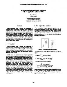


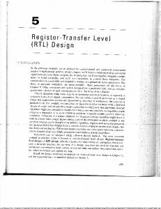


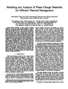


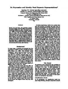


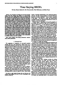
![ModelSim Tutorial - UCSD CSE [PDF]](https://m.moam.info/img/260x300/modelsim-tutorial-ucsd-cse-pdf_64799306098a9e495b8b45ed.jpg)