Neuro-symbolic EDA-based Optimisation using ILP-enhanced DBNs

Neuro-symbolic EDA-based Optimisation using ILP-enhanced DBNs

arXiv:1612.06528v1 [cs.AI] 20 Dec 2016

Sarmimala Saikia TCS Research, New Delhi [email protected]

Gautam Shroff TCS Research, New Delhi [email protected]

Lovekesh Vig TCS Research, New Delhi [email protected]

Puneet Agarwal TCS Research, New Delhi [email protected]

Ashwin Srinivasan Department of Computer Science BITS Goa [email protected] Richa Rawat TCS Research, New Delhi [email protected]

Abstract We investigate solving discrete optimisation problems using the ‘estimation of distribution’ (EDA) approach via a novel combination of deep belief networks (DBN) and inductive logic programming (ILP). While DBNs are used to learn the structure of successively ‘better’ feasible solutions, ILP enables the incorporation of domain-based background knowledge related to the goodness of solutions. Recent work showed that ILP could be an effective way to use domain knowledge in an EDA scenario. However, in a purely ILP-based EDA, sampling successive populations is either inefficient or not straightforward. In our Neuro-symbolic EDA, an ILP engine is used to construct a model for good solutions using domain-based background knowledge. These rules are introduced as Boolean features in the last hidden layer of DBNs used for EDA-based optimization. This incorporation of logical ILP features requires some changes while training and sampling from DBNs: (a) our DBNs need to be trained with data for units at the input layer as well as some units in an otherwise hidden layer; and (b) we would like the samples generated to be drawn from instances entailed by the logical model. We demonstrate the viability of our approach on instances of two optimisation problems: predicting optimal depth-of-win for the KRK endgame, and job-shop scheduling. Our results are promising: (i) On each iteration of distribution estimation, samples obtained with an ILP-assisted DBN have a substantially greater proportion of good solutions than samples generated using a DBN without ILP features; and (ii) On termination of distribution estimation, samples obtained using an ILP-assisted DBN contain more near-optimal samples than samples from a DBN without ILP features. Taken together, these results suggest that the use of ILP-constructed theories could be useful for incorporating complex domain-knowledge into deep models for estimation of distribution based procedures.

1

Introduction

There are many real-world planning problems for which domain knowledge is qualitative, and not easily encoded in a form suitable for numerical optimisation. Here, for instance, are some guiding principles that are followed by the Australian Rail Track Corporation when scheduling trains: (1) If a healthy Train is running late, it should be given equal preference to other healthy Trains; (2) A higher priority train should be given preference to a lower priority train, provided the delay to the lower priority train is kept to a minimum; and so on. It is evident from this that train-scheduling may benefit from knowing if a train is healthy, what a trains priority is, and so on. But are priorities 30th Conference on Neural Information Processing Systems (NIPS 2016), Barcelona, Spain.

and train-health fixed, irrespective of the context? What values constitute acceptable delays to a low-priority train? Generating good train-schedules will require a combination of quantitative knowledge of train running times and qualitative knowledge about the train in isolation, and in relation to other trains. In this paper, we propose a heuristic search method, that comes under the broad category of an estimation distribution algorithm (EDA). EDAs iteratively generate better solutions for the optimisation problem using machine-constructed models. Usually EDAs have used generative probabilistic models, such as Bayesian Networks, where domain-knowledge needs to be translated into prior distributions and/or network topology. In this paper, we are concerned with problems for which such a translation is not evident. Our interest in ILP is that it presents perhaps one of the most flexible ways to use domain-knowledge when constructing models. Recent work has shown that ILP models incorporating background knowledge were able to generate better quality solutions in each EDA iteration [14]. However, efficient sampling is not straightforward and ILP is unable to utilize the discovery of high level features as efficiently as deep generative models. While neural models have been used for optimization [15], in this paper we attempt to combine the sampling and feature discovery power of deep generative models with the background knowledge captured by ILP for optimization problems that require domain knowledge. The rule based features discovered by the ILP engine are appended to the higher layers of a Deep Belief Network(DBN) while training. A subset of the features are then clamped on while sampling to generate samples consistent with the rules. This results in consistently improved sampling which has a cascading positive effect on successive iterations of EDA based optimization procedure. The rest of the paper is organised as follows. Section 2 provides a brief description of the EDA method we use for optimisation problems. Section 2.1 describes how ILP can be used within the iterative loop of an EDA for discovering rules that would distinguish good samples from bad. Section 3 Describes how RBMs can be used to generate samples that conform to the rules discovered by the ILP engine. Section 4 describes an empirical evaluation demonstrating the improvement in the discovery of optimal solutions, followed by conclusions in Section 5.

2

EDA for optimization

The basic EDA approach we use is the one proposed by the MIMIC algorithm [4]. Assuming that we are looking to minimise an objective function F (x), where x is an instance from some instance-space X , the approach first constructs an appropriate machine-learning model to discriminate between samples of lower and higher value, i.e., F (x) ≤ θ and F (x) > θ, and then generates samples using this model Procedure EODS: Evolutionary Optimisation using DBNs for Sampling 1. Initialize population P := {xi }; θ := θ0 2. while not converged do (a) for all xi in P label(xi ) := 1 if F (xi ) ≤ θ else label(xi ) := 0 (b) train DBN M to discriminate between 1 and 0 labels i.e., P (x : label(x) = 1|M ) > P (x : label(x) = 0|M ) (c) regenerate P by repeated sampling using model M (d) reduce threshold θ 3. return P

Figure 1: Evolutionary optimisation using a network model to generate samples. Here we use Deep Belief Networks (DBNs) [7] for modeling our data distribution, and for generating samples for each iteration of MIMIC. Deep Belief Nets (DBNs) are generative models that are composed of multiple latent variable models called Restricted Boltzman Machines (RBMs).In particular, as part of our larger optimization algorithm, we wish to repeatedly train and then sample from the trained DBN in order to reinitialize our sample population for the next iteration as outlined in Figure 1. In order to accomplish this, while training we append a single binary unit (variable) to the highest hidden layer of the DBN, and assign it a value 1 when the value of the sample is below θ and a value 0 if the value is above θ. During training that this variable, which we refer to as the separator variable, learns to discriminate between good and bad samples. To sample from the DBN we additionally clamp our separator variable to 1 so as to bias the network to produce good samples, 2

and preserve the DBN weights from the previous MIMIC iteration to be used as the initial weights for the subsequent iteration. This prevents retraining on the same data repeatedly as the training data for one iteration subsumes the samples from the previous iteration. We now look at how ILP models can assist DBNs constructed for this purpose.

3 3.1

EDA using ILP-assisted DBNs ILP

The field of Inductive Logic Programming (ILP) has made steady progress over the past two and half decades, in advancing the theory, implementation and application of logic-based relational learning. A characteristic of this form of machine-learning is that data, domain knowledge and models are usually—but not always—expressed in a subset of first-order logic, namely logic programs. Sidestepping for the moment the question “why logic programs?”, domain knowledge (called background knowledge in the ILP literature) can be encodings of heuristics, rules-of-thumb, constraints, text-book knowledge and so on. It is evident that the use of some variant of first-order logic enable the automatic construction of models that use relations (used here in the formal sense of a truth value assignment to n-tuples). Our interest here is in a form of relational learning concerned with the identification of functions (again used formally, in the sense of being a uniquely defined relation) whose domain is the set of instances in the data. An example is the construction of new features for data analysis based on existing relations (“f (m) = 1 if a molecule m has 3 or more benzene rings fused together otherwise f (m) = 0”: here concepts like benzene rings and connectivity of rings are generic relations provided in background knowledge). There is now a growing body of research that suggests that ILP-constructed relational features can substantially improve the predictive power of a statistical model (see, for example: [9, 11, 12, 10, 13]). Most of this work has concerned itself with discriminatory models, although there have been cases where they have been incorporated within generative models. In this paper, we are interested in their use within a deep network model used for generating samples in an EDA for optimisation in Procedure EODS in Fig. 1. 3.2

ILP-assisted DBNs

Given some data instances x drawn from a set of instances X and domain-specific background knowledge, let us assume the ILP engine will be used to construct a model for discriminating between two classes (for simplicity, called good and bad). The ILP engine constructs a model for good instances using rules of the form hj : Class(x, good) ← Cpj (x).1 Cpj : X 7→ {0, 1} denotes a “context predicate”. A context predicate corresponds to a conjunction of literals that evaluates to T RU E (1) or F ALSE (0) for any element of X . For meaningful features we will usually require that a Cpj contain at least one literal; in logical terms, we therefore require the corresponding hj to be definite clauses with at least two literals. A rule hj : Class(x, good) ← Cpj (x), is converted to a feature fj using a one-to-one mapping as follows: fj (x) = 1 iff Cpj (x) = 1 (and 0 otherwise). We will denote this function as F eature. Thus F eature(hj ) = fj , F eature−1 (fj ) = hj . We will also sometimes refer to F eatures(H) = {f : h ∈ H and f = F eature(h)} and Rules(F ) = {h : f ∈ F and h = F eatures−1 (f )}. Each rule in an ILP model is thus converted to a single Boolean feature, and the model will result in a set of Boolean features. Turning now to the EODS procedure in Fig. 1, we will construct ILP models for discriminating between F (x) ≤ θ) (good) and F (x) > θ (bad). Conceptually, we treat the ILP-features as high-level features for a deep belief network, and we append the data layer of the highest level RBM with the values of the ILP-features for each sample as shown in Fig 2. 1 We note that in general for ILP x need not be restricted to a single object and can consist of arbitrary tuples of objects and rules constructed by the ILP engine would more generally be hj : Class(hx1 , x2 , . . . , xn i, c) ← Cpj (hx1 , x2 , . . . , xn i). But we do not require rules of this kind here.

3

(a)

(b)

Figure 2: Sampling from a DBN (a) with just a separator variable (b) with ILP features 3.3

Sampling from the Logical Model

Recent work [14] suggests that if samples can be drawn from the success-set of the ILP-constructed model2 then the efficiency of identifying near-optimal solutions could be significantly enhanced. A straightforward approach of achieving this with an ILP-assisted DBN would appear to be to clamp all the ILP-features, since this would bias the the samples from the network to sample from the intersection of the success-sets of the corresponding rules (it is evident that instances in the intersection are guaranteed to be in the success-set sought). However this will end up being unduly restrictive, since samples sought are not ones that satisfy all rules, but at least one rule in the model. The obvious modification would be to clamp subsets of features. But not all samples from a subset of features may be appropriate. With a subset of features clamped, there is an additional complication that arises due to the stochastic nature of the DBN’s hidden units. This makes it possible for the DBN’s unit corresponding to a logical feature fj to have the value 1 for an instance xi , but for xi not to be entailed by the background knowledge and logical rule hj . In turn, this means that for a feature-subset with values clamped, samples may be generated from outside the success-set of corresponding rules involved. Given background knowledge B, we say a sample instance x generated by clamping a set of features F is aligned to H = Rules(F ), iff B ∧ H |= x (that is, x is entailed by B and H). A procedure to bias sampling of instances from the success-set of the logical model constructed by ILP is shown in Fig. 3.

4

Empirical Evaluation

4.1

Aims

Our aims in the empirical evaluation are to investigate the following conjectures: (1) On each iteration, the EODS procedure will yield better samples with ILP features than without (2) On termination, the EODS procedure will yield more near-optimal instances with ILP features than without. (3) Both procedures do better than random sampling from the initial training set. It is relevant here to clarify what the comparisons are intended in the statements above. Conjecture (1) is essentially a statement about the gain in precision obtained by using ILP features. Let us denote 2

These are the instances entailed by the model along with the background knowledge, which—assuming the rules are not recursive—we take to be the union of the success-sets of the individual rules in the model.

4

Given: Background knowledge B; a set of rules H = {h1 , h2 , . . . , hN }l; a DBN with F = {f1 , f2 , . . . , fN } as high-level features (fi = F eature(hi )); and a sample size M Return: A set of samples {x1 , x2 , . . . , xM } drawn from the success-set of B ∧ H. 1. S := ∅, k = 0 2. while |k| ≤ N do (a) Randomly select a subset Fk of size k features from F (b) Generate a small sample set X clamping features in Fk (c) for each sample in x ∈ X and each rule hj , set countk = 0 i. if x ∈ success-set where (fj (x) = 1) => (x ∈ success-set(B and hj )) countk = countk + 1 3. Generate S by clamping k features where countk = max(count1 , count2 ...countN ) 4. return S Figure 3: A procedure to generate samples aligned to a logical model H constructed by an ILP engine.

P r(F (x) ≤ θ) the probability of generating an instance x with cost at most θ without ILP features to guide sampling, and by P r(F (x) ≤ θ|Mk,B ) the probability of obtaining such an instance with ILP features Mk,B obtained on iteration k of the EODS procedure using some domain-knowledge B. (note if Mk,B = ∅, then we will mean P r(F (x) ≤ θ|Mk,B ) = P r(F (x) ≤ θ)). Then for (1) to hold, we would require P r(F (x) ≤ θk |Mk,B ) > P r(F (x) ≤ θk ). given some relevant B. We will estimate the probability on the lhs from the sample generated using the model, and the probability on the rhs from the datasets provided. Conjecture (2) is related to the gain in recall obtained by using the model, although it is more practical to examine actual numbers of near-optimal instances (true-positives in the usual terminology). We will compare the numbers of near-optimal in the sample generated by the DBN model with ILP features, to those obtained using the DBN alone. 4.2 4.2.1

Materials Data

We use two synthetic datasets, one arising from the KRK chess endgame (an endgame with just White King, White Rook and Black King on the board), and the other a restricted, but nevertheless hard 5 × 5 job-shop scheduling (scheduling 5 jobs taking varying lengths of time onto 5 machines, each capable of processing just one task at a time). The optimisation problem we examine for the KRK endgame is to predict the depth-of-win with optimal play [1]. Although aspect of the endgame has not been as popular in ILP as task of predicting “White-to-move position is illegal” [2], it offers a number of advantages as a Drosophila for optimisation problems of the kind we are interested. First, as with other chess endgames, KRKwin is a complex, enumerable domain for which there is complete, noise-free data. Second, optimal “costs” are known for all data instances. Third, the problem has been studied by chess-experts at least since Torres y Quevado built a machine, in 1910, capable of playing the KRK endgame. This has resulted in a substantial amount of domain-specific knowledge. We direct the reader to [3] for the history of automated methods for the KRK-endgame. For us, it suffices to treat the problem as a form of optimisation, with the cost being the depth-of-win with Black-to-move, assuming minimax-optimal play. In principle, there are 643 ≈ 260, 000 possible positions for the KRK endgame, not all legal. Removing illegal positions, and redundancies arising from symmetries of the board reduces the size of the instance space to about 28, 000 and the distribution shown in Fig. 4(a). The sampling task here is to generate instances with depth-of-win equal to 0. Simple random sampling has a probability of about 1/1000 of generating such an instance once redundancies are removed. The job-shop scheduling problem is less controlled than the chess endgame, but is nevertheless representative of many real-life applications (like scheduling trains), and in general, is known to be computationally hard. 5

Cost Instances 0 27 (0.001) 1 78 (0.004) 2 246 (0.012) 3 81 (0.152) 4 198 (0.022) 5 471 (0.039) 6 592 (0.060) 7 683 (0.084) 8 1433 (0.136) Total Instances: 28056

Cost 9 10 11 12 13 14 15 16 draw

Instances 1712 (0.196) 1985 (0.267) 2854 (0.368) 3597 (0.497) 4194 (0.646) 4553 (0.808) 2166 (0.886) 390 (0.899) 2796 (1.0)

Cost Instances 400–500 10 (0.0001) 500–600 294 (0.003) 600–700 2186 (0.025) 700–800 7744 (0.102) 800–900 16398 (0.266) 900–1000 24135 (0.508) Total Instances: 100000

(a) Chess

Cost 1000–1100 1100–1200 1200–1300 1300–1400 1400–1500 1500–1700

Instances 24067 (0.748) 15913 (0.907) 7025 (0.978) 1818 (0.996) 345 (0.999) 66 (1.0)

(b) Job-Shop

Figure 4: Distribution of cost values. The number in parentheses are cumulative frequencies.

Data instances for Chess are in the form of 6-tuples, representing the rank and file (X and Y values) of the 3 pieces involved. For the RBM, these are encoded as 48 dimensional binary vector where every eight bits represents a one hot encoding of the pieces’ rank or file. At each iteration k of the EODS procedure, some instances with depth-of-win ≤ θk and the rest with depth-of-win > θk are used to construct the ILP model, and the resulting features are appended to train the RBM model as described in Section 3.2.3 Data instances for Job-Shop are in the form of schedules, with associated start- and end-times for each task on a machine, along with the total cost of the schedule. On iteration i of the EODS procedure, models are to be constructed to predict if the cost of schedule will be ≤ θi or otherwise.4 4.2.2

Background Knowledge

For Chess, background predicates encode the following (WK denotes the White King, WR the White Rook, and BK the Black King): (a) Distance between pieces WK-BK, WK-BK, WK-WR; (b) File and distance patterns: WR-BK, WK-WR, WK-BK; (c) “Alignment distance”: WR-BK; (d) Adjacency patterns: WK-WR, WK-BK, WR-BK; (e) “Between” patterns: WR between WK and BK, WK between WR and BK, BK between WK and WR; (f) Distance to closest edge: BK; (g) Distance to closest corner: BK; (h) Distance to centre: WK; and (i) Inter-piece patterns: Kings in opposition, Kings almost-in-opposition, L-shaped pattern. We direct the reader to [3] for the history of using these concepts, and their definitions. A sample rule generated for Depth θk . Use the features learnt by the ILP model to guide the DBN sampling. 3. Compute the ratio of P r(F (x) ≤ θk |Mk,B ) to P (F (x) ≤ θk ) The following details are relevant: • The sequence of thresholds for Chess are h8, 4, 2, 0i. For Job-Shop, this sequence is h900, 890, 880...600i; Thus, θ∗ = 0 for Chess and 600 for Job-Shop, which means we require exactly optimal solutions for Chess. • Experience with the use of ILP engine used here (Aleph) suggests that the most sensitive parameter is the one defining a lower-bound on the precision of acceptable clauses (the minacc setting in Aleph). We report experimental results obtained with minacc = 0.7, which has been used in previous experiments with the KRK dataset. The background knowledge for Job-Shop does not appear to be sufficiently powerful to allow the identification of good theories with short clauses. That is, the usual Aleph setting of upto 4 literals per clause leaves most of the training data ungeneralised. We therefore allow an upper-bound of upto 10 literals for Job-Shop, with a corresponding increase in the number of search nodes to 10000 (Chess uses the default setting of 4 and 5000 for these parameters). • In the EODS procedure, the initial sample is obtained using a uniform distribution over all instances. Let us call this P0 . On the first iteration of EODS (k = 1), the datasets E1 + and E1 − are obtained by computing the (actual) costs for instances in P0 , and an ILP model M1,B , or simply M1 , constructed. A DBN model is constructed both with and without ILP features. We obtained samples from the DBN with CD6 or by running the Gibbs chain for six iterations. On each iteration k, an estimate of P r(F (x) ≤ θk ) can be obtained from the empirical frequency distribution of instances with values ≤ θk and > θk . For the synthetic problems here, these estimates are in Fig. 4. For P r(F (x) ≤ θk |Mk,B ), we use obtain the frequency of F (x) ≤ θk in Pk • Readers will recognise that the ratio of P r(F (x) ≤ θk |Mk,B ) to P (F (x) ≤ θk ) is equivalent to computing the gain in precision obtained by using an ILP model over a non-ILP model. Specifically, if this ratio is approximately 1, then there is no value in using the ILP model. The probabilities computed also provide one way of estimating sampling efficiency of the models (the higher the probability, the fewer samples will be needed to obtain an instance x with F (x) ≤ θk ). 4.4

Results

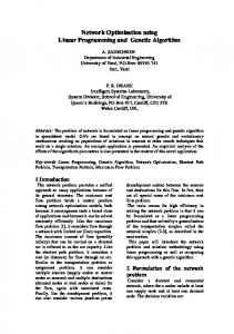
Results relevant to conjectures (1) and (2) are tabulated in Fig. 5 and Fig. 6. The principal conclusions that can drawn from the results are these: (1) For both problems, and every threshold value θk , the probabilty of obtaining instances with cost at most θk with ILP-guided RBM sampling is substantially higher than without ILP. This provides evidence that ILP-guided DBN sampling results in better samples than DBN sampling alone(Conjecture 1); (2) For both problems and every threshold value θk , samples obtained with ILP-guided sampling contain a substantially higher number of near-optimal instances than samples obtained using a DBN alone (Conjecture 2) Additionally, Fig. 7 demonstrates the cumulative impact of ILP on (a) the distribution of good solutions obtained and (b)the cascading improvement over the DBN alone for the Job Shop problem. The DBN with ILP was able to arrive at the optimal solution within 10 iterations. 7

Model None

k=1 0.134

DBN

0.220

DBNILP

0.345

P r(F (x) ≤ θk |Mk ) k=2 k=3 k=4 0.042 0.0008 0.0005

Model None

k=1 0.040

P r(F (x) ≤ θk |Mk ) k=2 k=3 k=4 0.036 0.029 0.024

0.050

0.015

0.0008

DBN

0.209

0.234

0.248

0.264

0.111

0.101

0.0016

DBNILP

0.256

0.259

0.268

0.296

(b) Job-Shop

(a) Chess

Figure 5: Probabilities of obtaining good instances x for each iteration k of the EODS procedure. That is, the column k = 1 denotes P (F (x) ≤ θ1 after iteration 1; the column k = 2 denotes P (F (x) ≤ θ2 after iteration 2 and so on. In effect, this is an estimate of the precision when predicting F (x) ≤ θk . “None” in the model column stands for probabilities of the instances, corresponding to simple random sampling (Mk = ∅). Model DBN DBNILP

Model

Near-Optimal Instances k=1 k=2 k=3 k=4 5/27 11/27 11/27 12/27 3/27

17/27

21/27

DBN DBNILP

22/27

Near-Optimal Instances k = 11 k = 12 k = 13 7/304 10/304 18/304 9/304

18/304

27/304

(b) Job-Shop

(a) Chess ∗

Figure 6: Fraction of near-optimal instances (F (x) ≤ θ ) generated on each iteration of EODS. In effect, this is an estimate of the recall (true-positive rate, or sensitivity) when predicting F (x) ≤ θ∗ . The fraction a/b denotes that a instances of b are generated.

(b) (a)

Figure 7: Impact of ILP on EODS procedure for Job Shop (a) Distribution of solution Endtimes generated on iterations 1, 5, 10 and 13 with and without ILP (b) Cumulative semi-optimal solutions obtained with and without ILP features over 13 iterations

5

Conclusions and Future Work

In this paper we demonstrate that DBNs can be used as efficient samplers for EDA style optimization approaches. We further look at combining the sampling and feature discovery power of Deep Belief Networks with the background knowledge discovered by an ILP engine, with a view towards optimization problems that entail some degree of domain information. The optimization is performed iteratively via an EDA mechanism and empirical results demonstrate the value of incorporating ILP based features into the DBN. In the future we intend to combine ILP based background rules with more sophisticated deep generative models proposed recently [5, 6] and look at incorporating the rules directly into the cost function as in [8]. 8

References [1] M. Bain and S. Muggleton. Learning optimal chess strategies. In K. Furukawa, D. Michie, and S. Muggleton, editors, Machine Intelligence 13, pages 291–309. Oxford University Press, Inc., New York, NY, USA, 1995. [2] Michael Bain. Learning logical exceptions in chess, 1994. PhD Thesis, University of Strathclyde. [3] Gabriel Breda. KRK Chess Endgame Database Knowledge Extraction and Compression, 2006. Diploma Thesis, Technische Universität, Darmstadt. [4] Jeremy S De Bonet, Charles L Isbell, Paul Viola, et al. Mimic: Finding optima by estimating probability densities. Advances in neural information processing systems, pages 424–430, 1997. [5] Danihelka I. Mnih A. Blundell C. Gregor, K. and D. Wierstra. Deep autoregressive networks. In ICML, 2014. [6] Danihelka I. Mnih A. Blundell C. Gregor, K. and D. Wierstra. D. draw: A recurrent neural network for image generation. In ICML, 2015. [7] Geoffrey Hinton. Deep belief nets. In Encyclopedia of Machine Learning, pages 267–269. Springer, 2011. [8] Zhiting Hu, Xuezhe Ma, Zhengzhong Liu, Eduard Hovy, and Eric Xing. Harnessing deep neural networks with logic rules. arXiv preprint arXiv:1603.06318, 2016. [9] Sachindra Joshi, Ganesh Ramakrishnan, and Ashwin Srinivasan. Feature construction using theory-guided sampling and randomised search. In ILP, pages 140–157, 2008. [10] Ganesh Ramakrishnan, Sachindra Joshi, Sreeram Balakrishnan, and Ashwin Srinivasan. Using ILP to construct features for information extraction from semi-structured text. In ILP, pages 211–224, 2007. [11] Amrita Saha, Ashwin Srinivasan, and Ganesh Ramakrishnan. What kinds of relational features are useful for statistical learning? In ILP, 2012. [12] Lucia Specia, Ashwin Srinivasan, Sachindra Joshi, Ganesh Ramakrishnan, and Maria Graças Volpe Nunes. An investigation into feature construction to assist word sense disambiguation. Machine Learning, 76(1):109–136, 2009. [13] Lucia Specia, Ashwin Srinivasan, Ganesh Ramakrishnan, and Maria das Graças Volpe Nunes. Word sense disambiguation using inductive logic programming. In ILP, pages 409–423, 2006. [14] Ashwin Srinivasan, Gautam Shroff, Lovekesh Vig, Sarmimala Saikia, and Puneet Agarwal. Generation of near-optimal solutions using ilp-guided sampling. In ILP. 2016. [15] Oriol Vinyals, Meire Fortunato, and Navdeep Jaitly. Pointer networks. In Advances in Neural Information Processing Systems, pages 2692–2700, 2015.

9