1
Neuromorphic Excitable Maps for Visual Processing C. Rasche Department of Psychology, The Pennsylvania State University, PA University Park, PA 16802 email:
[email protected]
to appear in IEEE Transactions on Neural Networks
Abstract— An excitable membrane is described which can perform different visual tasks such as contour detection, contour propagation, image segmentation and motion detection. The membrane is designed to fit into a neuromorphic multi-chip system. It consists of a single two-dimensional layer of locally connected integrate-andfire neurons and propagates input in the sub-threshold and the above-threshold range. It requires adjustment of only one parameter to switch between between the visual tasks. The performance of two spiking membranes of different connectivity is compared, a hexagonally and an octagonally connected membrane. Their hardware and system suitability is discussed.
Topic Area: Image Processing and Recognition Keywords: wave propagation, contour propagation, contour detection, motion detection, image segmentation
It will be shown that an excitable map can be adjusted such, that it acts as a contour detection mechanisms. In some sense, that is what certain silicon retinae already perform [9], [10], [11], [12]. For instance, the retina by Mahowald and Mead [9] detects the contours of a moving stimulus. Whereas their retina generated only analog output values, more recent silicon retinae, such as Boahen’s version [10], generate also a spiking output suitable for a multi-chip system. The contour detection process presented here shows the important difference that it can occur using a still-image, an issue hardly addressed in computational neuroscience. Other map properties will be shown, which are useful for other visual computations. It is then discussed how these maps may form part of a neuromorphic multi-chip system.
I. I NTRODUCTION a) : An excitable membrane is a two-dimensional sheet of neurons which propagates activity to all directions. It has been employed to model motion detection phenomena [1], motion speed estimation [2], contour detection in gray-scale images and contour propagation for shape recognition networks [3], [4], [5]. Glaser and Barch’s ’Excitable Neuronal Array’ employs non-spiking units [1]. In contrast, the here presented membrane, also called map, consists of spiking units, which allow 1) for a wider range of propagation properties and 2) for the possibility to emulate the maps in a neuromorphic multichip system (e.g. [6], [7], see [8] for alternative architectures). Neuromorphic multi-chip systems communicate by exchanging spikes and the output of an excitable map has therefore to represent a spiking format. Here, two variants of such a spiking membrane are presented: their propagation properties are characterized and their suitability for an analog hardware implementation and orientation extraction is discussed.
II. M ETHODS b) Map connectivity: A map consists of a 2D grid of neural units, each unit horizontally connected to its immediate neighbors by resistors. In a hexagonal grid, hereafter called the hex-grid, the neurons of every 2nd row (or column) are shifted by half the unit-spacing (as compared to the oct-grid) and each neuron is connected to its six neighbors (figure 1a, [shift in row shown]). This is also the preferred connectivity for two-dimensional (2D) electrotonic propagation, because it allows for even propagation and it is therefore easy to tune [13]. This hex-grid is one connectivity variant. But we also investigate another variant, an octagonally connected grid (the oct-grid, figure 1b), because it offers some advantages over the hex-grid. An octagonal grid is more difficult to tune but if one uses unidirectional resistors then it becomes robust. In the oct-grid, the neurons are aligned within an orthogonal coordinate system and each unit connects to its eight neighbors (figure 1b).
2
8 6
a
1
1
2
c
b
during spike wave propagation:
c c 5
2
7
3
when t = ton + dts : V = EK f or dtr .
(4)
This set of equations (1 to 4) fully describes the map’s dynamics and roughly represent the dynamics as they Fig. 1. Connectivity for the discussed maps (a-c). a. Hex-grid: a unit would occur if the map was implemented in a neu’c’ has 6 neighbors. b. Oct-grid: a unit ’c’ has eight direct neighbors romorphic system [13], [7] (see also discussion). In (not all horizontal connections shown). c. Oct-grid with unidirectional connections (only connections to the center unit are shown). previous literature the term ’wave’ was used to describe the traveling activity of waves of decreasing amplitude [13]. The sub-threshold behavior described in equations c) General dynamics: A neuron is modeled as 1 and 2 corresponds to that term. Because in the present an I&F unit (see e.g. [14]). Instead of simulating the study the focus lies on the propagation of spiking waves neuronal voltage and current dynamics explicitly, we - for which all equations are involved -, the term wave is merely model an activity variable, V , corresponding to only used for this actively propagating operating modus. the neuronal membrane potential. In the sub-threshold An alternative expression could be traveling wave. d) Parameter values and tuning: EN A , EK and domain (V < Vthres [spiking threshold]), the activity V thres are set to values 5.0, 0.0 and 2.0, respectively level of a neuron at location (x,y) at the next time step in accordance to voltage values often chosen in analog t + 1, is given by its present activity level plus the circuits (e.g. [13]). The simulation time step is set to a input Ih (t) of its neighboring neurons via the horizontal value of 0.2 and can be interpreted as milliseconds. dts connections: and dtr are set between 0.6 and 1.2, also interpretable V (x, y, t+1) = V (x, y, t)+Ih (t)+Iext , f or V < Vthres , as milliseconds. dts is usually set to a value of 1.0, (1) which would correspond to the general pulse width whereby Iext represents external input to the map. The in neuromorphic systems [6]. The map then requires term Ih consists of the sum of activity differences for the adjustment of only two more parameters, the axial each of the N neighboring neurons, multiplied by the conductance gh and the refractory period dtr . Given the value of dts , there exists a minimum value for dtr , which axial (or horizontal) conductance gh : is required to be slightly larger than the value for dts , N X Ih (t) = gh (Vk (t) − Vc (t)), (2) in order to ensure spike wave propagation without the bounce back of activity. The only parameter that then k=1 requires tuning is gh , which is generally set between where Vc is the activity level of the center neuron and 0.04 and 0.18 depending on the specific application. Vk is the activity level of the neighboring neurons. The e) Hexagonal grid (hex-grid): In the hex-grid, the two map variants, oct-grid and hex-grid, differ basically neighboring input I is as described in equation 2, with h in their term Ih (t). N being equal the 6 immediate neighbors. When horizontal (synaptic) or external input drives f) Octagonal grid (oct-grid): In an oct-grid, spike V above the spiking threshold Vthres , then a spike of wave propagation is uneven, because during outward duration dts is triggered - registered at time ton - during propagation of a point-source for example, the diagonal which the activity level is clamped to a maximum value, directions (toward units 2,4,6,8 in figure 1a) do not EN A , representing the reversal potential for sodium: receive the same amount of input as the lateral units when V > Vthres : ton = t, V = EN A f or dts , (3) (toward units 1,3,5,7). One can attempt to alleviate the problem by giving a higher conductance value to the During this ’high state’, the activity level will signifi- diagonal connections but this map variant is generally cantly contribute to its neighbors due to the large differ- difficult to tune, for example achieving stable spike wave ence in equation 2 and that may cause the neighboring propagation is intricate, and that is why this specific units to spike as well. This can lead to initiation of a version is not discussed any further. However, a variant spike wave. Following the high state, the activity level of the oct-grid connectivity provides robust spike wave is reset to a minimum value EK for a short while dtr propagation: this variant assumes that activity flows starting at t = ton + dts . EK represents the reversal only toward the lower side, an unidirectional connection potential for potassium. This ’low state’ serves as a (figure 1c). For this specific oct-grid version Ih is the refractory period prohibiting the bounce back of activity sum of positive membrane differences multiplied by the 4
3
6
5
4
3
Ih (t) = gh
8 X
max[(Vk (t) − Vc (t)), 0],
(5)
k=1
Because of this unidirectional flow, there is no decay of activity in this map: Input will integrate and never fade away unless a spike occurs, which would reset the unit; or unless a leakage conductance is added to a unit. g) Contour detection: The maps can be used to detect contours in a gray-scale image. This has already been shown for the oct-grid [3] but is here shown to work also for the hex-grid. It is assumed that the proposed edge detection process takes place in two stages: in a first stage, the image intensity distribution (gray-scale image) determines the activity level and spiking threshold of the excitable membrane. In a second stage, the activity level starts spreading in the sub-threshold domain and that eventually will trigger spikes where there is a large difference - a contrast edge - between two neuronal activity levels. The first stage is mimicked as follows. The image intensity distribution, I(x, y) (0 black, 255 white), is scaled to a range between values 0 and 4.0, denoted as Is . Is is then assigned to the activity level of the map at time 0: V (x, y, 0) = Is (x, y) (or: Iext = Is (x, y) at t=0; Iext = 0 for t>0). In addition, the threshold value of each neuron is individually adjustable and set above the individual activity level of each unit by a constant c: Vthres (x, y) = V (x, y, 0) + c. Given an offset of c = 0.5, the spiking thresholds would vary from 0.5 to 4.5 as opposed to the fixed threshold of 2.0 in the ’regular’ map. In the second stage, the activity level is propagated according to equations 1 to 4. Firstly, the activity will propagate in the sub-threshold domain (equations 1 and 2), which eventually will trigger spikes at high-contrast edges. Once spikes are triggered, the above-threshold equations come into play (equations 3 and 4) and the contours start propagating as a spiking wave. A biophysical motivation and discussion of this process can be found in [3]. h) Motion detection: The excitable maps can also be used to detect a moving input. This is not related to the contour detection mechanism and represents a different operation modus of the map. To transform the map to a motion-sensitive modus, the value for the horizontal conductance is decreased rendering the map’s dynamics inert as opposed to the propagation modi discussed above: for instance, a unit that spikes will not trigger spike wave propagation; the map will
only react repeatedly if there is continuous input along a certain direction - a motion input. Because there is no activity decay in the oct-grid version simulated here, such motion input can raise this map’s activity to a level where it causes excessive spiking. To prevent that, a leakage term L is introduced to each unit: equation 1 becomes V (x, y, t + 1) = V (x, y, t)+Ih (t)+Iext −L. We hereafter refer to this as the leaky oct-grid. The leakage conductance is chosen to be fixed for reason of simplicity - it can be implemented with a single transistor in analog hardware. To test this map, the following type of motion stimulus is employed: a series of input spikes stimulates the map from left to right. The input spikes are assumed to arrive from another chip, such as a silicon retina generating spikes in response to observed contours (e.g. [10]). The spikes would be fed to synaptic circuits in the corresponding neurons and trigger an excitatory postsynaptic potential (EPSP). In this simulation, the EPSP is emulated as a pulse-shaped response of amplitude a and a duration of a single time step: Iext (xs , ys , ts ) = a, with xs , ys and ts being selected locations and time steps that correspond to the motion stimulus. i) : When we discuss the general propagation properties in the subsequent section, we refer to three maps: 1) the hex-grid; 2) the oct-grid; or non-leaky oct-grid; 3) the leaky oct-grid, which is the oct-grid used for motion detection. 3 high g, low L low g, low L high g, high L low g, high L 2.5
2
activity
axial conductance, gh , for each of its 8 neighboring neurons:
1.5
1
0.5
0
0
1
2
3 space
4
5
6
Fig. 2. Sub-threshold propagation for the leaky oct-grid. 4 cases are plotted with a combination of two values (high and low) for the horizontal conductance and the leakage conductance. high gh =0.12; low gh =0.04; high L=0.16; low L=0.08. Y-axis: activity level; X-axis: space: neuronal unit number.
III. R ESULTS j) Sub-threshold behavior: The value of gh determines the rate of decay in time and space (the
4
time and space constant) [13], [14]. In the hex-grid either decay occurs exponential [13]. For the leaky oct-grid, the propagation properties are different and they are non-linear due to the specific connectivity pattern and the fixed leakage. Figure 2 illustrates the spatial decay for combinations of low and high values for both the leakage and the axial conductance: The spatial decay is generally slower as compared to an exponential decay. The temporal decay is constant due to the fixed leakage conductance. In contrast to those maps, for the non-leaky oct-grid (in which there is no decay) the axial conductance rather determines how fast the map builds up activity. In summary: decay in space decay in time hex-grid ∝ gh (exp) ∝ gh (exp) leaky oct-grid ∝ gh , L (non-lin) = L (const) (non-leaky) none (build up) none (build up) oct-grid hex−grid
t=1
10
10
20
20 5
t=5
20
20 10
15
20
10
20
20 10
15
20
10
20
20 15
20
10
20
20 5
10
15
20
15
20
5
10
15
20
5
10
15
20
5
10
15
20
5
10
15
20
5
10
15
20
20 10
15
20
10 20 10
15
20
10 20 5
10
10
10
5
10
10
20
5
10
leaky oct−grid
10
5
10
5
t=17
15
20
5
t=13
10
10
5
t=9
oct−grid
10
15
20
10 20 5
10
15
20
Fig. 3. Above-threshold propagation of a pixel source in a 20x20 map. Black pixels represent spiking units, gray pixels represent units with sub-threshold activity above 0. Left column: hex-grid (gh =0.12; ww ≈ 1.8). Middle column: oct-grid (gh =0.06; ww ≈ 1.2). Right column: leaky oct-grid (gh =0.12; L=0.08; ww ≈ 2.0). Snapshots of V at time steps 1,5,9,13 and 17 are shown. For both grids: dts =1.0; dtr =1.2. Partly reprinted with permission from Springer [5].
k) (Spike) wave propagation: The properties of spike wave propagation were firstly tested using a pixel source that is turned on for a single time step and that is large enough (above EN A ) so that it triggers an outwardgrowing annular wave. dts is set to a value of 1.0; dtr is set to a value slightly larger, 1.2, to prohibit the bounce back of activity. It is then only gh that needs some adjustment. Hex-grid: There exists a minimum value for gh (≈0.105) that will trigger the annular wave. Around
this minimal value the wave width ww extends more than one neuronal unit, meaning that two neighboring neurons will be active simultaneously for a short period (figure 3, left column). The hex-grid pattern is plotted in a regular orthogonal grid, which means that every 2nd row is shifted by half a unit. The contours for a hex-grid can therefore look aliased: this can be best understood in figure 4 for a vertical line. The wave speed ws is about one third of a neuronal unit. Increasing the value for gh increases both, wave width and wave speed. A change in spike duration dts modulates the wave width and does so more significantly than a change of gh , but it does not change wave speed. A decrease in Vthres increases wave width and wave speed, because units at the wave front exceed the spiking threshold earlier and because the activity difference across units (equation 2) is larger. An increase in Vthres has the reverse effect. Oct-grid: The above discussed effects of parameter changes for the hex-grid basically apply to the oct-grid as well, for both the leaky and the nonleaky version. The minimal wave speed is slightly higher - approximately half a unit per time step than for the hex grid. For the leaky version, the wave width and wave speed are inversely proportional to the value of L because it determines subthreshold integration time (figure 2). In summary: wave width, ww wave speed, ws hex-grid ∝ gh , 1/Vthres , ∝ gh , 1/Vthres dts leaky oct- ∝ gh , 1/Vthres , ∝ gh , 1/Vthres , grid 1/L, dts 1/L (non-leaky) ∝ gh , 1/Vthres , ∝ gh , 1/Vthres oct-grid dts For the hex-grid, the outward-propagating wave is exactly annular; for the oct-grid it is near annular and for larger values of gh (≈ 0.18) the wave becomes diamondshaped. Changing dtr also influences the wave width but its effects are minor as compared to the summarized parameter changes. l) Waxing and waning propagation: A piece of contour can be propagated in two modi. In one mode, a contour piece can trigger an outward-growing propagation wave. This mode has already been shown in figure 3 for the point source, and it is hereafter called the ’waxing’ mode. It is shown again in figure 4 for a vertical line (1st and 3rd column for the hex-grid and leaky oct-grid respectively). The waxing propagation can fill gaps in a contour image by mere propagation, which will be shown for contour detection. In the other mode, the contour propagates but gradually diminishes and this is referred to as the ’waning’ mode (2nd and 4th
5
hex−grid
hex−grid
t=1
leaky oct−grid
octagonal grid
leaky oct−grid
10
10
10
10
50
20
20
20
20
100
10
20
10
20
10
20
10
hexagonal grid
50 Photo
20
150 t=5
10
10
10
10
20
20
20
20
10
20
10
20
10
20
150 50
10
100
150
200
250
10
10
20
10
20 10
20
10
20 10
20
20
10
20
t=1
150
10
20
10
20 10
20
20
20 10
100
150
200
10
10
20
20
20
20
10
20
50
20
10
20
50
100
150
200
250
50
100
150
200
250
50
100
150
200
250
50
100
150
200
250
50 t=2
100
10
150 10
250
100
250
100 t=17 10
200
10
20 10
150
150 50
t=13 10
100
50
100
20 10
50
20
50 t=9
100
150
20 10
20
10
20
Fig. 4. Propagation of a vertical line. 1st column: hex-grid, waxing propagation (gh =0.12). 2nd column: hex-grid, waning propagation (gh =0.07). 3rd column: leaky oct-grid, waxing propagation (gh =0.08; L=0.08). 4th column: leaky oct-grid, waning propagation (gh =0.08; L=0.38). For both grids: dts =1.0; dtr =1.2. Display same as in figure 3.
50
100
150
200
250
50
50
100
t=4
150
150 50
100
150
200
250
50
50
100
column in figure 4). The waning mode can be obtained by lowering the value for gh (below 0.1). In this mode a contour starts to shrink from its contour endpoints. A closed contour triggers an inward- and an outwardpropagating wave. The outward-propagating contour is broken up into pieces each of which shrinks: the inwardpropagating contour does not diminish because there are no endpoints that nourish the waning effect. In this mode, it is not possible to trigger propagation of a pixel-source. The non-leaky oct-grid can not provide waning propagation because no decay is modeled in that map variant. m) Contour detection: Figure 5 illustrates the contour detection mechanism. The top row shows the grayscale image of an object, a desk (plotted twice). The rows below depict how the contours evolve during the propagation process. For the oct-grid (left column) c was set to a value of 0.5, for the hex-grid (right column) the value was set a little lower, 0.3, because the decay of (sub-threshold) activity occurs faster in this map. There are a number of characteristics to this detection process: 1) High-contrast contours are signaled first, followed by lower-contrast contours, because a steep edge reaches the neighboring spiking threshold faster than a shallow edge. 2) A contour triggers a wave towards both sides as expected from the above simulations. If one of these contours travels across a darker area, then its wave width and wave speed is larger due to the larger difference in
100
t=6
150
100 150
50
100
150
200
250
Fig. 5. Contour detection with the excitable map. Left column: oct-grid (gh =0.11,c=0.5). Right column: hex-grid (gh =0.09,c=0.3). For both grids: dts =0.6; dtr =1.2. Snapshots of spiking activity only are shown at time steps 1, 2, 4 and 6 (no sub-threshold activity is displayed).
equation 2, which is equivalent to an increased value of gh . This can be seen at time steps 4 and 6 for the large dark area in the middle of the desk object and the triangular area in the lower right: for both areas, the width of the inward-propagating wave is larger and the ’opposing’ waves separate faster than other contours, like the contours between drawers. 3) The detected contours may propagate in a waxing manner, as it is the case for the oct-grid shown in the left column. For low values of gh , the contours are signaled but only propagation across the dark areas takes place. Other contours are not propagated further, and thus this does not exactly represent a waning propagation as stated above. There is no substantial difference in the contour detection process between the two grids: both grids detect most contours, which can suffice for an object hypothesis. For the given parameter set, the contour detection
6
mechanism perform possibly for all images with regular illumination. The study in [3] contains more examples for the oct-grid map. Figure 6 shows the result of the hex-grid for images containing ’fuzzy’ contours. The parameters are exactly the same as for the stimulation in figure 5 (the hex-grid). In the example of the tree, the signaled contour image is granular during the first four time steps due to the image texture. The contour image is then segmented by the (waxing) propagation of contour pieces. In the animal picture, the first four time steps return the clearest contour image, later it becomes unrecognizable. These pictures show that the detailed evolvement of the contour image is individual to each picture. Different values for the offset c change the amount of contours detected: a high value of c selects highercontrast contours only, a lower value includes lowercontrast contours (figure 7). For lower values wave width and speed is faster as discussed above.
A decrease in gh has already been applied in order to switch from waxing to waning propagation. For the motion-sensitive map, the value is decreased even more (smaller than 0.07). The motion stimulus drops a series of EPSP into a 10x20 map every 2nd time step, along row number 5, starting with column number 2. Figure 8 shows the response of a hex-grid, whereby snap-shots of every 2nd time step are taken until time step number 24. The EPSP amplitude is 1.9, so just below the height of the spiking threshold. The map responds with a growing mound of increasing diameter and amplitude. Once the mound’s amplitude has reached the spiking threshold (with the 3rd EPSP drop, see plot number 3 in 1st column), then the generated spike increases the diameter even further and helps to maintain continuous spiking with each successive EPSP drop of the motion stimulus. Results for the oct-grid have been presented somewhere else [2]. c=0.3
hexagonal grid
hexagonal grid
100
50 Photo 100
200
150 200
300 50
100
150
200
100
50
t=2
100
150
200
100
100
200
200
300
300
400
400
200
50
600
200
c=0.2
150
200
400
400
600
100 c=0.1
200
300 50
100
150
200
100
50
t=4
100
150
200
100
200
200
300
300
400
400
50 100 150
200
100
200
300 50
100
150
200
100
50
t=6
100
150
200
400
600
200
400
600
Fig. 7. Varying the offset (c) in the contour detection mechanism (hexgrid). Parameters are as in figure 5 and 6 except for c (0.3, 0.2, 0.1, respectively). Only time step number 4 is shown for each simulation.
50 100 150
200
200
200
300 50
100
150
200
100
50
t=8
100
150
200
50
IV. D ISCUSSION
100 150
200
200
300 50
100
150
200
50
100
150
200
Fig. 6. More contour detection examples with the hex-grid. Parameters are as in figure 5. Snapshots are taken at time steps 2, 4, 6 and 8.
n) Motion detection: In order to run the excitable map as a motion-sensitive map, the propagation dynamics are made inert by decreasing the value for gh .
o) : An excitable map was presented, which can perform different visual functions if tuned appropriately. To switch between some of the functions, only the horizontal conductance value has to be adjusted: the map can propagate contours in a waxing and a waning mode; it processes motion stimuli; and it can detect contours using adjustable spiking thresholds. Each of these mechanisms can be analyzed in greater detail. This would make sense once a specific map is implemented
7
into analog hardware. The present study shows the versatility of such a map and that with either map (octgrid or hex-grid) the same effects can be generated. The choice of grid depends on the application and is discussed subsequently.
t=2
2 4 6 8 10
t=4
2 4 6 8 10
2 4 t=14 6 8 10 5
t=6
t=8
2 4 6 8 10
15
20
5
10
15
20
5
10
15
20
5
10
15
20
5
10
15
20
5
10
15
20
5
10
15
20
2 4 t=16 6 8 10 5
2 4 6 8 10
10
10
15
20 2 4 t=18 6 8 10
5
10
15
20 2 4 t=20 6 8 10
5
10
15
20
2 4 t=10 6 8 10
2 4 t=22 6 8 10 5
10
15
20
2 4 t=12 6 8 10
2 4 t=24 6 8 10 5
10
15
20
Fig. 8. Motion detection with the hex-grid (gh =0.03). Excitatory post-synaptic potentials are ’dropped’ from left to right. Black: spiking activity; gray: sub-threshold activity. Left column: snap shots starting at time step 2, continuing every 2nd time step. Right column: continuation of left column.
p) Contour detection: The contour output is adjustable by a single parameter, the offset c. Once adjusted, the contour detection mechanism operates on many images with ’normal’ luminance distributions. This is similar to computer vision algorithms (e.g. [15]), which also operate on many images once the appropriate parameters have been choosen. The network is therefore as robust as any algorithm generating contour images. But of course there always exist some images in which the luminance distribution is uneven enough, such that the fixed parameters do not capture the essential contours - whether this is a computer vision algorithm or the pre-
sented network. An importance difference to computer vision algorithms is that the presented network generates the contour image dynamically. How a visual system can deal with that is discussed later. q) Analog hardware suitability: 1. Excitable map. The currently existing silicon retinae consist of hexagonal (passive) maps made of a variety of resistor types [9], [7]. To render those excitable, some spiking mechanism had to be inserted which does not only sense the membrane voltage, but which would also contribute to its neighboring units when a spike occurs. This may be intricate for some of those maps, but a resistor variant that has already been tested for such dynamics are the switched capacitor circuits [16], [17]. Specifically, the study by Rasche and Douglas uses a spiking mechanism, which would cause back-propagation of a (somatic) spike signal into the neighboring compartments of a dendritic tree. The circuitry of that spiking mechanism is large because it emulates the sodium and potassium conductance, but simpler spiking mechanisms, e.g. a mere I&F neuron, may suffice as well. The equations in this study correspond most closely to the use of such a map. The shortcoming of this method is that it requires a fast clock and that renders the implementation rather a mixed analog-digital circuit using also more power than pure analog circuits. An oct-grid has not been implemented yet and would pose the problem of constructing uni-directional resistors. One could achieve that using follower-connected amplifiers, which however require much design space. 2. Contour detection. To ensure that the first stage occurs before the second stage starts, it may be necessary to inhibit the lateral propagation initially. In case of the switched capacitors, one way to ensure this inhibition would be to stop the clocks. To implement the individual adjustment of the spiking thresholds, a follower with offset could be used, which would set the threshold voltage, but which would be turned off as soon as the second stage starts. r) Embedding into a multi-chip system: 1. Contour processing. Because the contour image is generated dynamically (e.g. figure 6) subsequent processing had to deal with this dynamic output in some way. One may think of stabilizing or ’snatching’ the contours in some way, but one may also render subsequent integration dynamics slower, e.g. the integrating neurons would possess large time constants (slowly decaying excitatory post-synaptic potentials). An alternative would be to employ the propagation directly for region encoding, see item 2 next. A future goal is to extract the local orientation of
8
propagation waves from such maps as it has already been done for certain recognition architectures [4], [18]. The hex-grid offers 6 orientations (3 ’unaliased’ and 3 aliased) per ’elementary’ subfield (figure 1b). But due to the existent alternation of the wave front into one direction (figure 3), a higher resolution is necessary to distinguish between orientations. In contrast, the octgrid offers 8 orientations (4 unaliased and 4 aliased) per elementary subfield and those orientations do not alternate into a given propagation direction. Thus, the oct-grid allows for a larger number of orientations per subfield and can be easily used to compute directionselectivity, whereas for the hex-grid one had to chose a higher resolution to obtain the same robust orientation measures. 2. Region processing. The main purpose of contour propagation is the encoding of regions, as for example used in Blum’s symmetric-axis transform [19]. A neuromorphic plausible architecture of this process has already been implemented [4]. The system used the presented propagation map to propagate the contours and during this propagation process the fragmented contours would simply fuse. In that specific simulation, the starting point for propagation was the contour image obtained from a computer vision algorithm. A next step would be to demonstrate the operation of the transform with the presented contour detection mechanism, but for such a single continuous system to work, one had to adjust the orientation detectors in that system (see paragraph above). Furthermore, in that simulation the kind of propagation was of the waxing ’unlimited’ type, which possesses the advantage of closing gaps in a contour image. It also can lead to segmentation if the inside of a shape contains contour pieces from texture. But the downside of this process is that noisy contour streaks can also perturb the proper development of those symmetric axes. An alternative would be to use waning propagation, which represents a ’controlled’ propagation. Using that form of propagation, small contour pieces which can result from speckled noise - are given less importance. However, the symmetric axes would not be fully generated and subsequent processing had to take that into account. 3. Speed estimation and detecting flow patterns. The propagation maps could also be used to estimate speed. Different maps tuned to different, inert dynamics would detect different motion speeds: a motion speed would then be signaled by the activity of a specific map or a combination of them [2]. The advantage of this form of speed estimation is that it is independent of a directional read-out. Another value of these inert map dynamics lies
in exploring the use of different strength values for the individual connections. This was already exploited in a study where such motion-sensitive maps served to store certain flow patterns [18]. In both applications, the input to such maps would come from a silicon retinae or the here presented contour detection mechanism. 4. Segmentation. In computer vision, the processes of image segmentation and texture segregation are often carried out using different filter sizes (e.g [20]) which is size costly if one would attempt to transform them into a neuromorphic multi-chip system. The segmentation process shown in figure 6 does not compare to those elaborate and refined computer studies, but it shows that the excitable map can principally perform this process using only a sheet of interconnected neurons. It remained to be worked out of course, whether this principal can be extended to for example segregate the textures as discussed in Malik and Perona’s study [20]. s) Biological plausibility: The biological plausibility of excitable membranes has already been exhaustively discussed in previous studies. A general justification of excitable membranes can be found in [1], [5], a justification of the individual mechanisms is given in the respective studies (e.g. [3], [4]). Here, the arguments are summarized in key words. Visual processing occurs blazingly fast [21], [22] and if propagating waves would be involved in recognition then they had to occur reasonably fast, for example on a time scale of tens of milliseconds. Fast waves have not been observed yet, they may however be difficult to detect [1]. Fast wave propagation may occur on a neuronal/map level as simulated here. The retina propagates waves by either the electrical gap junction coupling of ON bipolar cells [23], [24] or by coupling of horizontal cells (see [25] for a more detailed discussion). In the primary visual cortex such propagation has not been found yet, but there is also the possibility that waves are propagated at a more ’global’, neural signal, for instance at the population level in which thousands of neurons would represent a small patch of the excitable membrane [26]. Because the excitable maps do not make use of any specific neural code, such as rate or synchronization code, one may wonder how realistic that aspect is. Again, given the high processing speed, it may be that single spikes are employed between maps, as it is implied in this study. Others have already proposed codes that compute with mere single spikes [27], [28], which belong to the class of timing codes. The excitable maps do not require any specific spike timing, they employ merely wave propagation and the generated spikes would be
9
projected to other maps. ACKNOWLEDGMENTS The study was carried out in Prof. Michael Wenger lab at the University of Notre Dame funded by a grant from the University Graduate School. The author wishes to thank Michael Wenger for generous support. R EFERENCES [1] D. Glaser and D. Barch, “Motion detection and characterization by an excitable membrane: The ’bow wave’ model,” Neurocomputing, vol. 26-7, no. jun, pp. 137–146, 1999. [2] C. Rasche, “Speed estimation with propagation maps,” Neurocomputing, vol. 69, pp. 1599–1607, 2005. [3] ——, “Signaling contours by neuromorphic wave propagation,” Biological Cybernetics, vol. 90, no. 4, pp. 272–279, 2004. [4] ——, “A neural architecture for the symmetric-axis transform,” Neurocomputing, vol. 64, pp. 301–317, 2005. [5] ——, The Making of a Neuromorphic Visual System. Berlin, Heidelberg, New York: Springer, 2005. [6] S. Deiss, R. Douglas, and A. Whatley, “A pulse-coded communications infrastructure for neuromorphic systems,” in Pulsed Neural Networks, W. Maass and C. M. Bishop, Eds. The MIT Press, 1999, ch. 6, pp. 157–178. [7] L. Shih-Chii, J. Kramer, G. Indiveri, T. Delbrueck, and R. Douglas, Analog VLSI: Circuits and Principles. Cambridge, MA: MIT Press, 2002. [8] E. Ros, E. Ortigosa, R. Agis, R. Carrillo, and M. Arnold, “Realtime computing platform for spiking neurons (rt-spike),” Neural Networks, IEEE Transactions on, vol. 17, no. 4, pp. 1050–1063, 2006. [9] M. Mahowald and C. Mead, “Silicon retina,” Scientific American, vol. 264(5), pp. 76–82, May 1991. [10] K. Boahen, “A retinomorphic chip with parallel pathways: Encoding increasing, on, decreasing, and off visual signals,” Analog Integr. Circuits Process., vol. 30, no. 2, pp. 121–135, 2002. [11] A. Z. Y. Murray, F. Worgotter, K. Cameron, and V. Boonsobhak, “A neuromorphic depth-from-motion vision model with stdp adaptation,” Neural Networks, IEEE Transactions on, vol. 17, no. 2, pp. 482–495, 2006. [12] S. Kameda and T. Yagi, “An analog silicon retina with multichip configuration,” Neural Networks, IEEE Transactions on, vol. 17, no. 1, pp. 197–210, 2006. [13] C. A. Mead, Analog VLSI and Neural Systems. Reading, Massachusetts: Addison-Wesley, 1989. [14] C. Koch, Computational Biophysics of Neurons. Cambridge:Mass.: MIT, 1999. [15] J. Canny, “A computational approach to edge-detection,” IEEE Transactions on Pattern Analysis and Machine Intelligence, vol. 8, no. 6, pp. 679–698, 1986. [16] J. G. Elias, “Artificial dendritic trees,” Neural Computation, vol. 5, pp. 648–664, 1993. [17] C. Rasche and R. Douglas, “Forward- and backpropagation in a silicon dendrite,” IEEE Transactions on Neural Networks, vol. 12, no. 2, pp. 386–393, 2001. [18] C. Rasche, “Visual shape recognition with contour propagation,” Biological Cybernetics, vol. 93, no. 1, pp. 31–42, 2005. [19] H. Blum, “Biological shape and visual science,” J Theor Biol, vol. 38(2), pp. 205–87, 1973. [20] J. Malik and P. Perona, “Preattentive texture-discrimination with early vision mechanisms,” J. Opt. Soc. Am. A-Opt. Image Sci. Vis., vol. 7, no. 5, pp. 923–932, 1990. [21] M. C. Potter, “Meaning in visual search,” Science, vol. 187, no. 4180, pp. 965–6, Mar 1975.
[22] S. Thorpe, D. Fize, and C. Marlot, “Speed of processing in the human visual system,” vol. 381, pp. 520–522, 1996. [23] S. Borges and M. Wilson, “The lateral spread of signal between bipolar cells of the tiger salamander retina,” BIOLOGICAL CYBERNETICS, vol. 63, no. 1, pp. 45–50, 1990. [24] W. Hare and W. Owen, “Receptive field of the retinal bipolar cell: A pharmacological study in the tiger salamander,” JOURNAL OF NEUROPHYSIOLOGY, vol. 76, no. 3, pp. 2005–2019, 1996. [25] A. Jacobs and F. Werblin, “Spatiotemporal patterns at the retinal output,” J. Neurophysiol., vol. 80, no. 1, pp. 447–451, 1998. [26] E. Rolls and G. Deco, Computational neuroscience of vision. New York: Oxford University Press, 2002. [27] S. J. Thorpe, “Spike arrival times: a highly efficient coding scheme for neural networks,” in Parallel Processing in Neural Systems and Computers, R. Eckmiller, G. Hartmann, and G. Hauske, Eds. Elsevier Science Publishers, 1990, pp. 91–94. [28] J. Hopfield, “Pattern recognition computation using action potential timing for stimulus representation,” Nature, vol. 376, pp. 33–36, 1995.
Christoph Rasche Christoph Rasche received a diploma in theoretical neurobiology at the University of Z¨urich in 1996. He completed a PhD degree in Computational Neuroscience, with a focus on Neuromorphic Engineering, at the ETH Z¨urich in 1999. During a postdoctoral stay in Christof Koch’s lab at Caltech, Pasadena, he began studying the subject of visual object recognition. He presently is in Karl Gegenfurtner’s lab at the University of Giessen (Germany) carrying out research in visual psychophysics. His research interests are investigating and modeling the visual recognition process and the development of a neuromorphic architecture for visual object and scene recognition. His research vision is layed out in a book called “The Making of a Neuromorphic Visual System” published with Springer.