Neuromorphic Hardware In The Loop: Training a Deep Spiking ... - arXiv

arXiv:1703.01909v1 [cs.NE] 6 Mar 2017

Neuromorphic Hardware In The Loop: Training a Deep Spiking Network on the BrainScaleS Wafer-Scale System Sebastian Schmitt† Johann Klähn† Guillaume Bellec§ Andreas Grübl† Maurice Güttler† Andreas Hartel† Stephan Hartmann‡ Dan Husmann† Kai Husmann† Sebastian Jeltsch† Vitali Karasenko† Mitja Kleider† Christoph Koke† Alexander Kononov† Christian Mauch† Eric Müller† Paul Müller† Johannes Partzsch‡ Mihai A. Petrovici†k Stefan Schiefer‡ Stefan Scholze‡ Vasilis Thanasoulis‡ Bernhard Vogginger‡ Robert Legenstein§ Wolfgang Maass§ Christian Mayr‡ René Schüffny‡ Johannes Schemmel† Karlheinz Meier† {sschmitt, kljohann, agruebl, gguettle, ahartel, husmann, khusmann, sjeltsch, vkarasen, mkleider, koke, akononov, cmauch, mueller, pmueller, mpedro, schemmel, meierk}@kip.uni-heidelberg.de {stephan.hartmann, johannes.partzsch, stefan.schiefer, stefan.scholze, vasileios.thanasoulis, bernhard.vogginger, christian.mayr, rene.schueffny}@tu-dresden.de {guillaume, robert.legenstein, maass}@igi.tugraz.at † Heidelberg ‡ Technische

University, Kirchhoff-Institute for Physics, Im Neuenheimer Feld 227, D-69120 Heidelberg Universität Dresden, Chair for Highly-Parallel VLSI-Systems and Neuromorphic Circuits, D-01062 Dresden § Graz University of Technology, Institute for Theoretical Computer Science, A-8010 Graz k University of Bern, Department of Physiology, Bühlplatz 5, CH-3012 Bern

Abstract—Emulating spiking neural networks on analog neuromorphic hardware offers several advantages over simulating them on conventional computers, particularly in terms of speed and energy consumption. However, this usually comes at the cost of reduced control over the dynamics of the emulated networks. In this paper, we demonstrate how iterative training of a hardware-emulated network can compensate for anomalies induced by the analog substrate. We first convert a deep neural network trained in software to a spiking network on the BrainScaleS wafer-scale neuromorphic system, thereby enabling an acceleration factor of 10 000 compared to the biological time domain. This mapping is followed by the in-the-loop training, where in each training step, the network activity is first recorded in hardware and then used to compute the parameter updates in software via backpropagation. An essential finding is that the parameter updates do not have to be precise, but only need to approximately follow the correct gradient, which simplifies the computation of updates. Using this approach, after only several tens of iterations, the spiking network shows an accuracy close to the ideal software-emulated prototype. The presented techniques show that deep spiking networks emulated on analog neuromorphic devices can attain good computational performance despite the inherent variations of the analog substrate.

I. I NTRODUCTION Recently, artificial neural networks (ANNs) have emerged as the dominant machine learning paradigm for many pattern recognition problems [1]. Although ANNs are to some extent inspired by the architecture of biological neuronal networks, they differ significantly from their biological counterpart in many respects. First, while the computation in biological neurons is performed through analog voltages in continuous time, ANNs are typically implemented on digital hardware

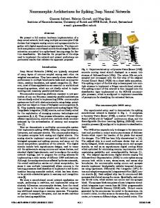
Fig. 1. The BrainScaleS system as it is currently installed consisting of five cabinets, each containing four neuromorphic wafer-scale systems. Upstream connectivity to the control cluster is provided by the prominent red cables, each communicating at Gigabit speed. This enables fast system configuration and high-throughput spike in- and output. An additional rack hosts the support infrastructure comprising power supplies, servers, the control cluster, and network equipment.

and thus operate in discretized time. Second, while the communication between neurons in an ANN is based on high-precision arithmetic and computed in discrete time steps, communication in biological neuronal networks is largely based on stereotypically shaped all-or-none voltage

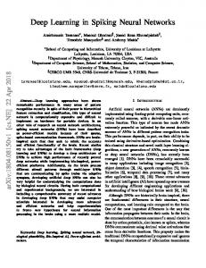
events in continuous time. These events are called action F potentials or spikes. In recent years, several large-scale analog G neuromorphic computing platforms have been developed [2] E G that better match these features of biological neural networks. I Due to their low power consumption and speedup compared to simulations run on conventional architectures, these systems are promising precursors for computing devices that can rival D C the computational capabilities and energy efficiency of the B A H human brain. H While spiking neural networks are in principle able to H emulate any ANN [3], it has been unclear whether neuromorphic hardware can be efficiently used to implement (a) (b) contemporary deep ANNs. One obstacle has been the lack of adequate training procedures. ANNs are typically trained by Fig. 2. (a) 3D-schematic of a BrainScaleS wafer module (dimensions: 50 cm × 50 cm × 15 cm) hosting the wafer (A) and 48 FPGAs (B). The positioning backpropagation, a learning algorithm that propagates high- mask (C) is used to align elastomeric connectors that link the wafer to the precision errors through the layers of the network. Recently the large main PCB (D). Support PCBs provide power supply (E & F) for the successful training of neural networks was demonstrated on on-wafer circuits as well as access (G) to analog dynamic variables such as neuron membrane voltages. The connectors for inter-wafer (USB slots) the TrueNorth chip, a fully digital spike-based neuromorphic and off-wafer/host connectivity (Gigabit-Ethernet slots) are distributed over design [4]. More specifically, performance on machine- all four edges (H) of the main PCB. Mechanical stability is provided by an learning benchmarks is not impaired by their hardware aluminum frame (I). (b) Photograph of a fully assembled wafer module. quantization constraints if, at each training step, the errors are computed with quantized parameters and binarized activations, Section III-A, we then describe the mapping of the neural before backpropagating with full precision. This advance network to the hardware, Section III-B. Subsequently, we however left the question open whether a similar strategy could describe the in-the-loop training in detail and demonstrate the be used for analog neuromorphic systems. Since TrueNorth is application of this procedure to a handwritten digit recognition fully digital, an exact software model is available. Therefore, task, Section III-C and Section IV. each parameter, neuron activations, and the corresponding gradients are available or can be appropriately approximated II. T HE B RAIN S CALE S WAFER -S CALE S YSTEM at any point in time during training. In contrast, the neural The BrainScaleS system follows the principle of so-called circuits on analog hardware are not as precisely controllable, “physical modeling”, wherein the dynamics of VLSI circuits making an exact mapping between the hardware and software are designed to emulate the dynamics of their biological domains challenging. archetypes instead of numerically computing them as in the In this work, we demonstrate the successful training of an conventional simulation approach of von Neumann archianalog neuromorphic system configured to implement a deep tectures. Neurons and synapses are implemented by analog neural architecture. The system we used is the BrainScaleS circuits that operate in continuous time, governed by time wafer-scale system, a mixed-signal neuromorphic architecture constants which arise from the properties of the transistors that features analog neuromorphic circuits with digital, event- and capacitors on the microelectronic substrate. In contrast to based communication. We implemented a training procedure real-time neuromorphic devices, see [8], the analog circuits similar to [4], but used only a coarse software model to on our system are designed to operate in a regime where approximate its behavior. We show that, nevertheless, the characteristic time constants (e.g., τ syn , τm ) are much smaller backpropagation algorithm is capable to adapt the synaptic than typical corresponding biological values. This defines our parameters of the neuromorphic network quite effectively intrinsic hardware acceleration factor of 10 000 with respect when running the training with the hardware in the loop. to biological real-time. The system is based on the ideas Similar approaches have already been used, in the context of described in [9] but in the meantime it has advanced from various network architectures, for smaller analog neuromor- a lab prototype to a larger installation comprising 20 wafer phic platforms, such as the HAGEN [5], [6] and Spikey [7] modules, see fig. 1. chips. For the parameter updates, we used the recorded activity A. The Wafer Module of the neuromorphic system, but computed the corresponding At the heart of the BrainScaleS wafer module, see fig. 2, is gradients using the parameters of the ANN. This adaptation a silicon wafer with 384 HICANN (High Input Count Analog was possible in spite of the fact that the algorithm had Neural Network) chips produced in 180 nm CMOS technology. no explicit knowledge about exact parameter values of the It comprises 48 reticles, each containing 8 HICANNs, that neurons and synapses in the BrainScaleS system. are connected in a post-processing step. Each chip hosts 512 The remainder of the article is structured as follows. neurons emulating Adaptive exponential integrate-and-fire In Section II, we describe the BrainScaleS neuromorphic (AdEx) dynamics [10], [11] being able to reproduce most of platform and discuss the extent of parameter variability in this the firing regimes discussed in [12]. When forming logical system. Starting from a simple approximate software model, neurons by combining up to 64 neuron circuits, a maximum

90

TABLE I H ARDWARE UTILIZATION AND POWER RATINGS FOR DIFFERENT NEURAL NETWORK ARCHITECTURES . MaxHW

384 22 445 4 030 000 13.6 Hz 10 000 550 GHz 3.6 nJ

384 196 608 43 253 760 40 Hz 10 000 17.3 THz 0.1 nJ

input from 14 080 conductance-based synapses is reached where each circuit contributes with 220 synapses. While the synapse and neuron dynamics are emulated by the analog circuits in continuous time, action potentials are transported as digital data packets [13]. The action potentials, or spikes, are injected asynchronously into circuit-switched routing structures on the chip and can be statically routed to target synapses and transported off-chip as time-stamped digital events via a packet-based network [14], [15]. 48 Xilinx Kintex-7 FPGAs, one per reticle, provide an I/O interface for configuration and spike data. The connection between FPGAs and the control cluster network is established using standard Gigabit and 10-Gigabit-Ethernet. Auxiliary PCBs provide the BrainScaleS wafer-scale system with power, control and analog readout. The specified maximum design power of a single module is 2 kW. This operating point (MaxHW) assumes an average spike rate of 40 Hz applied to all hardware synapses. As there are currently no power management techniques in use, all numbers reported in table I are based on the maximum design power. Table I also provides data regarding hardware utilization for previously published neural network architectures [16]. B. Running Neuronal Network Experiments The BrainScaleS software stack transforms a user-defined abstract neural network description, i.e., network topology, model parameters and input stimuli, to a corresponding hardware-constrained experiment configuration. Descriptions of spiking neural networks are often formulated using dedicated languages. Most are based on either declarative syntax, e.g., NineML [17] or NeuroML [18], or use procedural syntax, e.g., the Python-based API called PyNN [19]. The current BrainScaleS system uses PyNN to describe neural network experiments based on experiences with previous implementations [20]. This design choice enables the use of the versatile software packages developed in the PyNN ecosystem, such as the Connection Set Algebra [21], Elephant [22] or Neo [23]. Starting from the user-defined experiment description in PyNN, the transformation process maps model neurons to hardware circuits, routes connections between neurons to create synapses, and translates the model parameters to hardware settings. This translation of neuron and synapse

80 70

20

60 50

15 #

352 14 375 3 470 000 4.8 Hz 12 000 200 GHz 10 nJ

AI

synaptic time constant [ms]

HICANNs Neurons Synapses Average Rate (Bio) Speedup (Bio → HW) Total Rate (HW) Energy/Synaptic Event

L2/3

Network[16]

40 10

30 20

5

10 0

200 300 400 500 600 700 800 900 DAC

0 0 10

101 synaptic time constant [ms]

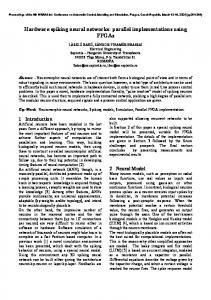
Fig. 3. Example for the calibration of the synaptic time constant. Left: measured synaptic time constants (y-axis) for different neurons as a function of the digital parameter (DAC, x-axis) controlling the responsible analog parameter. Right: measured synaptic time constant with (blue) and without (white) calibration for all neurons of a HICANN (right).

0 membrane potential [mV]

Model

Model[16]

25

−10 −20 −30 −40 −50

BrainScaleS Simulation 500

1000

1500 time [ms]

2000

2500

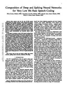
Fig. 4. Comparison of a recorded membrane trace to a neuron simulated with NEST. The neuron receives an excitatory Poisson stimulus of 20 Hz followed by inhibitory and then simultaneous excitatory and inhibitory Poisson stimuli of the same frequency. All calibrations are applied and the hardware response is converted to the emulated biological domains.

model parameters requires calibration data, see Section II-C, as well as rules for the conversion between the biological and the hardware time and voltage domains. The result of the whole transformation process is a hardware-compatible, abstract experiment description which can be converted into low-level configuration data. After acquiring hardware access using a fair resource scheduling and queuing system based on SLURM [24], the hardware is configured and the experiment is ready to run on the system. Although the BrainScaleS software stack provides a userfriendly modeling interface and hides hardware specifics, all low-level settings are available to the expert user. In particular the experiments presented here make use of this feature, enabling fast iterative modification of synaptic weights and input stimuli. C. Calibration For each neuron, the calibration provides translation rules from target parameters, such as the membrane time constant, to a set of corresponding hardware control parameters.

Thereby it accounts for circuit-to-circuit variations caused by the transistor mismatch inherent to the wafer manufacturing process. The data are stored in the hardware domains and two scaling rules are used for the conversion to the biological time and voltage domains. All time constants are scaled with the acceleration factor of 10 000, e.g., 1 µs hardware time corresponds to 10 ms of emulated biological time. Voltages are scaled according to Vhardware = Vbio × α + s,

input layer hidden layer

1

label layer

2 3 .. .

(1)

where α is a unit-free scaling factor and s is an offset. From here on, all units are given in the biological domain if not stated otherwise. Fig. 3 exemplifies the calibration technique for the particular case of the synaptic time constant. For every neuron, the analog parameter controlling the synaptic time constant is varied and the resulting synaptic time constant is determined from a recorded post-synaptic potential. A fit to this data then provides the mapping from the desired synaptic time constant to the value of the control parameter. Calibration reduces the neuron-to-neuron variation significantly, but not perfectly. The remaining variability is mostly caused by the trial-to-trial variation of the analog parameter storage. Fig. 4 shows two membrane time courses comparing a calibrated silicon neuron to a numerical simulation with NEST [25]. In both cases, the same model parameters and input spike trains were used. Despite the overall match, it can be seen that the calibration is not perfect, e.g. for the neuron used in fig. 4, the inhibitory stimulus is weaker compared to the expectation from simulation. Due to the analog nature of the system, variations will always occur to a certain extent, rendering in-the-loop training essential for networks that are sensitive to parameter noise, as we discuss in the following.

hidden layer

.. .

.. .

.. .

N −2 5 N −1 15

15

N 100 Fig. 5. Topology of the feed-forward neural network with one input layer, two hidden layers and one label layer. The dimension of the input layer is equal to the number of pixels of the input image. The number of label units is equal to the number of image classes the network is trained to recognize. 28

10

10

1.0

21

8

8

0.9

6

6

0.8

4

4

2

2

14 7 0

0

7

14

21

28

0

0

2

4

6

8

10

0

0.7 0.6 0

2

4

6

8

10

0.5

10

10

10

8

8

8

6

6

6

4

4

4

0.2

2

2

2

0.1

0.4 0.3

III. T RAINING A D EEP S PIKING N ETWORK 0 0 0 0.0 0 2 4 6 8 10 0 2 4 6 8 10 0 2 4 6 8 10 In the following, we describe our network model and training setup. Since we are using an abstract network of Fig. 6. Examples of the input data used during training. Original MNIST rectified linear units (ReLUs) and an equivalent spiking image of a “0” (upper left) vs. reduced-resolution image (lower left). Middle and right column: reduced-resolution images from the other four classes (“1”, network of leaky integrate-and-fire (LIF) neurons in parallel, “4”, “6”, “7”). we will first describe the networks structure in abstract terms. Our network is modeled as a feed-forward directed graph as shown in fig. 5. The input layer, consisting of 100 units, B. The resulting weights are converted to synaptic weights is used to represent the input patterns that the network later in an appropriately parametrized LIF network on the learns to classify. Each of these classes is represented by one BrainScaleS hardware. label unit. Between the input and label layers are two 15-unit C. The synaptic weights are further trained in a hardwarehidden layers that learn particular features in the input space. software training loop. The weights of the directed edges are learned during several phases of training, as described farther below. A. Software Model Our network was trained on a modified subset of the MNIST The training of the software model is performed similarly dataset of handwritten digits [26]. First, we decreased the to [27] using the TensorFlow [28] software with the properties resolution from 28 × 28 pixels to 10 × 10 pixels by bicubic detailed in the following. interpolation. To account for the lower dissimilarity of the 1) Input: The grayscale value of the input image pixels reduced resolution images, we restricted the dataset to the is transformed to a number between 0 and 1 and set as the five digit classes “0”, “1”, “4”, “6” and “7”. This results in a activation of the units in the input layer. training set of 30 690 and a test set of 5083 images. 2) Units: The output xk of ReLU unit k is given by The spiking neural network is then trained in three phases: X  A. The software model of the network with rectified linear xk = R Wkl xl , R(a) = max(0, a), (2) units (ReLUs) is trained with classical backpropagation. l

TABLE II N EURON PARAMETERS AND TYPICAL POST- CALIBRATION VARIATIONS . Parameter

Value

Inhibitory Reversal Potential Reset Potential Resting Potential Spike Threshold Excitatory Reversal Potential Inh./Exc. Synaptic Time Constant Membrane Time Constant

−80 mV −64 mV −40 mV −37.5 mV 0 mV 5 ms 20 ms

Relative Variation 5% 2% 10 % 0.5 % 0.5 % 10 % 10 %

where Wkl is the weight of the connection from unit l to unit k, R : R → R is the activation function of a ReLU, and the sum runs over all indices l of units from the previous layer. 3) Weights: The initial weights for layer n containing Nn units are drawn from a normal distribution with a mean of zero and standard deviation 1 , (3) σn = p Nn−1 where weight magnitudes > 2σn are dropped and re-picked. 4) Training: The network is trained by mini-batch gradientdescent with momentum [29] minimizing the cost function X X 2 2 1 C(W ) = 15 (˜ ys − y ˆs ) + (4) 2 λWkl , s∈S

kl

where W is the matrix containing all network weights, y ˆs the one-hot vector for the true digit, y ˜ = N2ndyhidden the scaled activity of the label layer and S the samples in the current batch of 100 samples. The first term in (4) is the euclidean distance between the predicted labels y ˜ and the true labels y ˆ, rewarding correct and penalizing wrong activity. The second term of (4) regularizes the weights with λ = 0.001, leading to the suppression of large weights to prevent overfitting. Per training step, the weights are updated according to ∆Wkl ← η∇Wkl C(W ) + γ∆Wkl , Wkl ← Wkl − ∆Wkl ,

(5) (6)

where ∆Wkl is the change in weight, η = 0.05 is learning rate, and γ = 0.9 the momentum parameter. In foresight of the hardware implementation, Wkl is clipped to [−1, 1]. B. Neuromorphic Implementation 1) Input: The input image is converted to Poisson spike trains following [30]: cp νp = P · νtot , (7) p cp where νp is the firing rate of the input corresponding to the pth pixel, cp the grayscale value of the pth pixel and νtot is the targeted total firing rate the input layer receives. In our case, we set νtot = 2500 Hz. Each pattern is presented for 0.9 s followed by 0.1 s of silence to allow the activity to decay.

2) Hardware Configuration: The network is mapped to the BrainScaleS hardware using the software stack detailed in Section II-B. Neurons of all layers, including the input layer, are randomly placed on 8 HICANNs. For input and on-wafer routing, 6 additional chips are used. These 14 HICANNs are connected to 5 different FPGAs. For each artificial neuron, four hardware neuron circuits are connected to form one logical neuron to increase the number of possible inputs. Except for the stimulus to the input layer, each pair of neurons in consecutive layers is connected with both an inhibitory and an excitatory synapse. This allows the weights to change sign during learning without having to change the configured topology. Therefore, the hardware-emulated network has a total of 3700 synapses. 3) Neuron parameters: Despite the different input and output domain, the activation functions of ReLUs and LIF neurons share features, i.e., both have a threshold below which the output is zero and a positive gradient for suprathreshold input. Not all neuron features are required to mimic the ReLU behavior, therefore we disable the adaptation and exponential features of the AdEx model. The parameters and the neuron-toneuron variation after calibration, see Section II-C, are listed in table II. To allow a balanced representation of positive and negative weights, the reversal potentials have been chosen as symmetric around the resting potential. The refractory period is set as small as possible to be close to a linear relation of the input to the output activity. Equation (1) is used to convert to hardware units with α = 20 and s = 1800 mV, e.g., the target value of the resting potential on hardware equals 1 V. 4) Weights: The trained weights Wkl of the artificial 0 network are converted to the 4 bit hardware weights Wkl by 0 Wkl = round(|Wkl | × 15). (8) Positive (negative) weights are assigned to excitatory (inhibitory) synapses and the corresponding inhibitory (excitatory) synapse is turned off. C. Hardware In The Loop Section III-B laid out the necessary steps to convert the artificial network to a network of neurons in analog hardware. After conversion it was found that the classification accuracy was significantly reduced compared to the initially trained ANN. To compensate for the reduced classification accuracy, training was continued with the hardware in the loop, see fig. 7. In-the-loop training consists of a series of training steps, each of which is performed as follows. First, the neuron activity is recorded for a batch of training samples. These firing rates are then equated to the ReLU unit response, where we used ˜ = 30yHz . The the following heuristic for the label layer: y resulting vector is used to compute the cost function C(W ) defined in (4). The weight updates are then computed using (5) using the ReLU activation function (2) as an approximation of the difficult-to-determine activation functions of the hardwareemulated neurons. For the experiments described here, we used the parameters η = 0.05, γ = 0 and a batch size of 1200 samples.

neuromorphic substrates. However, two non-trivial problems exist. First, the input-output relationship of the abstract backpropagation units used in typical deep networks needs to be mapped to spiking neuron dynamics. Second, in case of analog hardware, distortions in these dynamics need to be take into account. The latter is especially problematic because the performance weight updates ReLU activity of the network usually relies on precise parameter training. Here, we have addressed these problems in the context of the BrainScaleS wafer-scale system, an accelerated analog neuromorphic platform that emulates biologically inspired 4 bit weight discretization spikes neuron models. For mapping activities from the abstract domain to spikes, we have used a rate-coding scheme. The translation of the network topology, including connectivity structure and parameters, was described in Section III-B. prediction MNIST BrainScaleS Following this mapping of a pretrained network to the forward pass hardware substrate, the resulting distortions in dynamics and parameters have been compensated by in-the-loop training, Fig. 7. Illustration of our in-the-loop training procedure. In an antecedent as described in Section III-C. step (not shown), a software-trained ReLU network, see fig. 5, is mapped to This two-stage approach was evaluated for a small network an equivalent LIF network on the BrainScaleS hardware. Each iteration of in-the-loop training consists of two passes. In the forward pass, the output trained on handwritten digits. In this exemplary scenario, it firing rates of the LIF network are measured in hardware. In the backward was possible to almost completely restore the performance pass, these rates are used to update the synaptic weights of the LIF network of the software-simulated abstract model in hardware. An by computing the corresponding weight updates in the ReLU network and mapping them back to the hardware. implicit, but essential component of our methodology is the fact that the backpropagation of errors needs not be precise: computing the cost function gradients using a ReLU activation IV. R ESULTS function is sufficient for adapting the weights in the spiking An example for the activity on the neuromorphic hardware network. This circumvents the difficulty of otherwise having during classification after in-the-loop training for one choice to determine an exact derivative of the cost function with of hardware neurons and initial software parameters can be respect to the LIF activation function, which would be further found in fig. 10. The figure shows the spike times of all exacerbated by the diversity of neuronal activation functions neurons in the network for five presented samples of every on the analog substrate. digit. An image is considered to have been classified correctly Here, the mapping-induced distortions in network dynamics if the neuron associated with the input digit shows the highest and configuration parameters have been compensated by activity of all label neurons. After training, all images are additional training. A complementary approach would be correctly classified, except for the first example of digit “6” to modify the network in a way that makes it more robust which was mistaken for a “4”. Comparing the weights before to hardware-induced distortions, as discussed, e.g., in [16]. and after in-the-loop training, see fig. 8, shows that only slight While rate-based approaches such as ours are inherently robust adjustments are needed to compensate for hardware effects. against jitter in the timing of spikes, robust architectures The evolution of the accuracy per training batch for both the become particularly important in single-spike coding schemes, software model and the in-the-loop training of the hardware is as discussed in [31]. shown in fig. 9 for 130 different sets of hardware neurons and The proof-of-principle experiments presented here were initial weights of the software model. The total classification part of the commissioning phase of the BrainScaleS system accuracy is computed as the sum of correctly classified and lay the groundwork for more extensive studies. The patterns divided by the total number of patterns in the test most interesting question to be addressed next is whether set. After 15 000 training steps, the accuracy of the software the results achieved here also hold for larger networks that model is 97 % with a negligible uncertainty arising from the can deal with more complex datasets. Once fully functional, choice of initial weights. Directly after converting the artificial our system will be able to accomodate such large networks network to the network of spiking neurons, the accuracy is without any scaling-induced reduction in processing time due +12 +1 reduced to 72 −10 %. It increases to 95 −2 % at the end of the to its inherently parallel nature. in-the-loop training, being close to the performance of the In the long run, the potentially most rewarding challenge software model with the uncertainty given by the interquartile will be to fully port the training to the hardware as well. range (IQR). To this end, an integrated plasticity processor [32] has been designed that will allow the emulation of different learning V. D ISCUSSION rules at runtime [33]. Learning can then also profit from the For problems involving spatial pattern recognition, deep acceleration that, for now, only benefits the operation of the neural networks have become state of the art. Almost by fully trained network. The use of analog spiking hardware definition, they should lend themselves to implementation in might then not only allow accelerated data processing with backward pass

1.0

15

0.9

before in-the-loop

0.8 0.7 0.6 0

0.5 0.4 0.3 0.2 0.1

-15 -15

0 after in-the-loop

15

-15

0 after in-the-loop

15

-15

0 after in-the-loop

0.0

15

Fig. 8. Correlation of hardware weights before and after in-the-loop training for the projections to the first (left) and second hidden layer (center) and the label layer (right). Weights that are zero before and after training are omitted. The relative frequency is encoded by both grayscale and area of the corresponding square. 1.0

accuracy on training batch

0.9 0.8 0.7 0.6 0.5 0.4 0.3

software model

0.2 0.1

BrainScaleS

median, IQR 0 101

102

103

104

training step

median, IQR 0

5

10

15 20 25 in-the-loop iteration

30

35

Fig. 9. Classification accuracy per batch as a function of the training step for the software model (left) and the in-the-loop iteration for the hardware implementation (right) for 130 runs. The uncertainty, given by the interquartile range (IQR), expresses the variations when repeating the software model with different initial weights and the in-the-loop training using different initial weights for the ReLU training and different sets of hardware neurons.

pre-specified networks, but also facilitate fast training of biologically inspired architectures that can, in certain contexts, even outperform classical machine learning algorithms [34]. ACKNOWLEDGMENT This work has received funding from the European Union Sixth Framework Programme ([FP6/2002-2006]) under grant agreement no 15879 (FACETS), the European Union Seventh Framework Programme ([FP7/2007-2013]) under grant agreement no 604102 (HBP), 269921 (BrainScaleS) and 243914 (Brain-i-Nets) and the Horizon 2020 Framework Programme ([H2020/2014-2020]) under grant agreement no 720270 (HBP) as well as the Manfred Stärk Foundation. The authors wish to thank Simon Friedmann, Matthias Hock, Ioannis Kokkinos, Tobias Nonnenmacher, Lukas Pilz, Moritz Schilling, Dominik Schmidt, Sven Schrader, Simon Ziegler, and Holger Zoglauer for their contributions to the development and commissioning of the system, Würth Elektronik GmbH & Co. KG in Schopfheim for the development and manufacturing of the special wafer-carrier PCB used in the BrainScaleS wafer-scale system, and Fraunhofer-Institut für Zuverlässigkeit und Mikrointegration (IZM), Berlin, Germany

for developing the post-processing technique which is required for wafer-wide communication and external connectivity to the wafer. The first two authors contributed equally to this work. R EFERENCES [1] Y. LeCun, Y. Bengio, and G. Hinton, “Deep learning,” Nature, vol. 521, no. 7553, pp. 436–444, May 2015. [2] S. Furber, “Large-scale neuromorphic computing systems,” J Neural Eng, vol. 13, no. 5, p. 051001, 2016. [3] W. Maass, “Fast sigmoidal networks via spiking neurons,” Neural Comput, vol. 9, no. 2, pp. 279–304, 1997. [4] S. K. Esser, P. A. Merolla, J. V. Arthur et al., “Convolutional networks for fast, energy-efficient neuromorphic computing,” Proc. Natl. Acad. Sci. U.S.A., 2016. [5] S. G. Hohmann, J. Fieres, K. Meier et al., “Training fast mixed-signal neural networks for data classification,” in Proc Int Jt Conf Neural Netw, vol. 4. IEEE Press, Jul. 2004, pp. 2647–2652. [6] J. Fieres, J. Schemmel, and K. Meier, “A convolutional neural network tolerant of synaptic faults for low-power analog hardware,” in Proceedings of 2nd IAPR International Workshop on Artificial Neural Networks in Pattern Recognition, ser. Springer Lecture Notes in Artificial Intelligence, vol. 4087. Ulm, Germany: Springer International Publishing, Aug. 2006, pp. 122–132. [7] T. Pfeil, A. Grübl, S. Jeltsch et al., “Six networks on a universal neuromorphic computing substrate,” Frontiers in Neuroscience, vol. 7, p. 11, 2013.

X X X X X X

20

X X X X

time [s]

X

15

X X X X

10

X X X X X

5

X X X X

0

0

10

20

30

40 50 60 input layer

70

80

90

100

105 110 hidden layer

115

120 125 hidden layer

130 131 132 133 134 label layer

Fig. 10. Spike raster plot of the neural activity of all layers on the neuromorphic hardware after in-the-loop training. Each horizontal dash denotes the time at which a certain neuron spiked. Five examples per digit are presented where in the plot same digits are denoted by the same background color. Correctly classified images are marked with a green circle.

[8] S.-C. Liu, Event-based neuromorphic systems. John Wiley & Sons, 2015. [9] J. Schemmel, D. Brüderle, A. Grübl et al., “A wafer-scale neuromorphic hardware system for large-scale neural modeling,” in IEEE Int Symp Circuits Syst Proc, May 2010, pp. 1947–1950. [10] R. Brette and W. Gerstner, “Adaptive exponential integrate-and-fire model as an effective description of neuronal activity,” J. Neurophysiol., vol. 94, no. 5, pp. 3637–3642, 2005. [11] S. Millner, A. Grübl, K. Meier et al., “A VLSI implementation of the adaptive exponential integrate-and-fire neuron model,” in Adv Neur In, J. Lafferty, C. K. I. Williams, J. Shawe-Taylor et al., Eds., vol. 23, 2010, pp. 1642–1650. [12] R. Naud, N. Marcille, C. Clopath et al., “Firing patterns in the adaptive exponential integrate-and-fire model,” Biological Cybernetics, vol. 99, no. 4, pp. 335–347, Nov 2008. [Online]. Available: http://dx.doi.org/10.1007/s00422-008-0264-7 [13] J. Schemmel, J. Fieres, and K. Meier, “Wafer-scale integration of analog neural networks,” in Proc Int Jt Conf Neural Netw, Hong Kong, Jul. 2008. [14] V. Thanasoulis, B. Vogginger, J. Partzsch et al., “A pulse communication flow ready for accelerated neuromorphic experiments,” in IEEE Int Symp Circuits Syst Proc, Jun. 2014, pp. 265–268. [15] S. Scholze, S. Schiefer, J. Partzsch et al., “VLSI implementation of a 2.8 GEvent/s packet-based AER interface with routing and event sorting functionality,” Front Neurosci, vol. 5, p. 117, 2011. [16] M. A. Petrovici, B. Vogginger, P. Müller et al., “Characterization and compensation of network-level anomalies in mixed-signal neuromorphic modeling platforms,” PLoS ONE, vol. 9, no. 10, p. e108590, 2014. [17] I. Raikov, R. Cannon, R. Clewley et al., “NineML: the network interchange for neuroscience modeling language,” BMC Neuroscience, vol. 12, no. 1, p. P330, 2011. [18] P. Gleeson, S. Crook, R. C. Cannon et al., “NeuroML: A language for describing data driven models of neurons and networks with a high degree of biological detail,” PLoS Comput Biol, vol. 6, no. 6, p. e1000815, Jun. 2010. [19] A. P. Davison, D. Brüderle, J. Eppler et al., “PyNN: a common interface for neuronal network simulators,” Front Neuroinform, vol. 2, no. 11, 2008. [20] D. Brüderle, E. Müller, A. Davison et al., “Establishing a novel modeling tool: A python-based interface for a neuromorphic hardware system,” Front Neuroinform, vol. 3, no. 17, 2009.

[21] M. Djurfeldt, “The connection-set algebra—a novel formalism for the representation of connectivity structure in neuronal network models,” Neuroinformatics, vol. 10, no. 3, pp. 287–304, 2012. [22] M. Denker, A. Yegenoglu, D. Holstein et al., “elephant: An open-source tool for the analysis of electrophysiological data.” in Proceedings of the 11th Meeting of the German Neuroscience Society, Neuroforum 2015. German Neuroscience Society, Mar 2015, pp. T27–2B. [23] S. Garcia, D. Guarino, F. Jaillet et al., “Neo: an object model for handling electrophysiology data in multiple formats,” Front Neuroinform, vol. 8:10, February 2014. [24] M. Jette and M. Grondona, “SLURM: Simple linux utility for resource management,” in Proceedings of ClusterWorld Conference and Expo, San Jose, California, 2003. [25] M.-O. Gewaltig and M. Diesmann, “NEST (NEural Simulation Tool),” Scholarpedia, vol. 2, no. 4, p. 1430, 2007. [26] Y. LeCun and C. Cortes, “The MNIST database of handwritten digits,” 1998. [Online]. Available: http://yann.lecun.com/exdb/mnist [27] Y. Cao, Y. Chen, and D. Khosla, “Spiking deep convolutional neural networks for energy-efficient object recognition,” Int J Comput Vis, vol. 113, no. 1, pp. 54–66, 2015. [28] M. Abadi, A. Agarwal, P. Barham et al., “TensorFlow: Large-scale machine learning on heterogeneous systems,” Google Research, Whitepaper, 2015, software available from tensorflow.org. [Online]. Available: http://tensorflow.org/ [29] N. Qian, “On the momentum term in gradient descent learning algorithms,” Neural Netw., vol. 12, no. 1, pp. 145–151, 1999. [30] P. O’Connor, D. Neil, S.-C. Liu et al., “Real-time classification and sensor fusion with a spiking deep belief network,” Front Neurosci, vol. 7, p. 178, 2013. [31] M. A. Petrovici, A. Schroeder, O. Breitwieser et al., “Robustness from structure: fast inference on a neuromorphic device with hierarchical LIF networks,” submitted to IJCNN 2017, 2016. [32] S. Friedmann, “The Nux processor v3.0,” Electronic Vision(s) Group, Kirchhoff-Institute for Physics, Heidelberg University, User Guide, 2015. [Online]. Available: https://github.com/electronicvisions/nux [33] S. Friedmann, J. Schemmel, A. Grübl et al., “Demonstrating hybrid learning in a flexible neuromorphic hardware system,” IEEE Trans. Biomed. Circuits Syst., vol. PP, no. 99, pp. 1–15, 2016. [34] L. Leng, M. A. Petrovici, R. Martel et al., “Spiking neural networks as superior generative and discriminative models,” in Cosyne Abstracts, Salt Lake City USA, February 2016.