fact that all domains of neighbouring variables w have to be revised against the domain of v. ..... are cheap can MAC-3d get away with this. AVL trees do not ...
Queue Representation for Arc Consistency Algorithms M.R.C. van Dongen and D. Mehta Boole Centre for Research in Informatics/Cork Constraint Computation Centre University College Cork
Abstract. Arc consistency algorithms are an indispensable tool for efficiently solving many problems arising in computer science, mathematics, and the real world. Coarse-grained algorithms like AC-2001, AC-3, and AC-3d are efficient when it comes to saving time. Revision ordering heuristics for selecting arcs or variables from a data structure called a queue have a major impact on the average performance of these algorithms. This paper demonstrates that queue representation also plays an important role. We study a vqueue (queue containing variables) based on lists and aqueues (queues containing arcs) based on lists, linear probing, and AVL trees. Aqueues based on lists prove the least efficient and vqueues prove the most efficient for saving time. Vqueues result in more checks but less time because of the small overhead of queue maintenance. We experimentally compare MAC-3, MAC-3d , and MAC-2001. For random problems vqueues enable the algorithms to solve about 4 times faster on average than aqueues based on lists. With a vqueue MAC-3 becomes the fastest solver on average.
1
Introduction
Arc consistency algorithms are an indispensable tool for efficiently solving many problems arising in computer science, mathematics, and the real world. Coarse-grained arc consistency algorithms like AC-3 [7], AC-3d [10], and AC-2001 [1] are efficient for saving time. Revision ordering heuristics for selecting arcs or variables from a data structure called a queue have a major impact on the average performance of such algorithms [6, 10–12]. The traditional approach to minimising time is to avoid repeating checks. This paper demonstrates that queue representation also plays a significant role. We investigate several approaches to organising queues containing arcs (aqueues) and variables (vqueues): a vqueue based on lists and aqueues based on lists, on linear probing, and on AVL trees. We theoretically and experimentally compare the time complexity of queue representation. Our analysis demonstrates that an aqueue based on lists is the least efficient and that a vqueue based on lists is the most efficient for saving time. Experimental results agree with our theoretical analysis. For random problems vqueues enable the algorithms to solve about 4 times faster on average than aqueues based on lists. With a vqueue MAC-3 becomes the quickest solver on average. Compared to MAC-2001 it becomes about 1.22 times faster for random problems and becomes the quickest solver of most real-world problems. This is an important result because MAC-3 repeats its checks whereas MAC-2001, at the price of a much higher space complexity, does not.
This paper is organised as follows. Section 2.1 conists of a brief introduction to the constraint paradigm, to notation for describing veriable and arc selection heuristics, and and the arc consistency algorithms under consideration. Section 3 reviews the queue representation literature. Section 4 describes the four queue representations and presents a theoretical comparison. Section 5 presents experimental results. Conclusions are presented in Section 6.
2
Preliminaries
2.1 Constraint Satisfaction A binary constraint Cxy between variables x and y is a subset of the Cartesian product of the domains D(x) of x and D(y) of y. A value v ∈ D(x) is supported by w ∈ D(y) if ( v, w ) ∈ Cxy . Similarly, w ∈ D(y) is supported by v ∈ D(x) if ( v, w ) ∈ Cxy . A Constraint Satisfaction Problem (CSP) is a tuple ( X, D, C ), where X is a set containing n variables, D is a function mapping each variable x ∈ X to its domain, and C is a set containing e constraints between variables in subsets of X. We only consider CSPs whose constraints are binary. CSP ( X, D, C ) is called arc-consistent if its domains are non-empty and for each Cxy ∈ C it is true that every v ∈ D(x) is supported by y and that every w ∈ D(y) is supported by x. A support check (consistency check) is a test to find out if two values support each other. The tightness of the constraint Cxy between x and y is defined as 1−| Cxy |/(| D(x) |× | D(y) |). The density of ( X, D, C ) is defined as 2e/(n2 − n), for n > 1. The degree of a variable is the number of constraints involving that variable. MAC-X is a backtracker that uses algorithm AC-X for maintaining arc-consistency during search. 2.2
Defining Selection Operators
In this section we briefly recall the notation from [11] for describing and “composing” variable and arc selection operators. The composition of order �2 and linear quasi-order �1 is denoted �2 • �1 . It is the unique order defined as follows: v �2 • �1 w ⇐⇒ (v �1 w ∧ ¬w �1 v) ∨ (v �1 w ∧ w �1 v ∧ v �2 w) . In words, �2 • �1 uses �1 and “breaks ties” using �2 . Composition associates to the left: �3 • �2 • �1 is equal to (�3 • �2 ) • �1 . The result of lifting linear quasi-order � and function f is denoted ⊗f� . It is the linear quasi-order such that v ⊗f� w if and only if f (v) � f (w). Let πi (( v1 , . . . , vn )) = vi denote the i-th projection operator. Definition 1 (Projective Order). Let 1 ≤ i ≤ 2, let f (( x1 , x2 )) be a function only depending on xi , and let g(( x1 , x2 )) be a function not depending on xi . If ⊗f�1 and ⊗g�2 define orders then ⊗g�2 • ⊗f�1 is called a projective order. The order is primary projective if i = 1 and secondary projective if i = 2.
Example 1. Let #(v) ≤ #(w) if and only if variable v is lexicographically less than #◦π2 #◦π1 or equal to variable w. The lexicographical order ⊗≤ • ⊗≤ and the reverse lex#◦π1 #◦π2 icographical order ⊗≤ • ⊗≤ are arc selection operators. The former is primary projective and the latter is secondary projective. To compare two arcs, the primary (secondary) projective order first uses the first (second) members of these arc to decide the relative ordering between the two arcs. Only in the event of ties will it use the second (first) members of these arcs to break these ties. 2.3
AC-3 Based Arc Consistency Algorithms
In 1977, Mackworth presented an arc-consistency algorithm called AC-3 [7]. AC-3 has � a O ed3 bound for its worst-case time complexity [8]. AC-3 has a O (e + nd) space complexity. AC-3 cannot remember all its checks. Pseudo code for AC-3 and for the revise algorithm upon which it depends is depicted in Figures 1 and 2. The “For Each s ∈ S Do statement” construct assigns the members in S to s from small to big and carries out statement after each assignment. AC-3 uses arc heuristics to repeatedly select and remove an arc, ( x, y ), from a data structure called a queue (a set, really) and uses the constraint between x and y to revise the domain of x. Here revising D(x) using the constraint between x and y means removing the values from D(x) that are not supported by y. AC-3’s arc heuristics determine the constraint that will be used for the next check. There are also domain heuristics. Given the constraint for the next check these heuristics determine the values that will be used for the next check. The interested reader is referred to [7, 8] for further information about AC-3.
Function � AC-3( X ) : Boolean; Q := ( x, y ) ∈ X 2 : x and y are neighbours ; Function revise(x, y, Var change x ) : Boolean; While Q 6= ∅ Do Begin Begin change x := False; select and remove any arc ( x, y ) from Q; If Not revise(x, y, change x ) Then For Each r ∈ D(x) Do If @c ∈ D(y) s.t. c supports r Then Begin Return False; Else If change x Then D(x) := D(x) \ { r }; change x := True; Q := Q ∪ { ( z, x ) : z 6= y, z is a neighbour of x }; End; End; Return True; Return D(x) 6= ∅; End; End;
Fig. 1. The AC-3 algorithm
Fig. 2. Algorithm revise
Wallace and Freuder pointed out that arc heuristics can influence the efficiency of arc-consistency algorithms [12]. Similar observations were made in [4, 6, 10, 11]. Bessi`ere and R´egin presented AC-2001 [1], which is based on AC-3. AC-2001 revises one domain at a time. The main difference between AC-3 and AC-2001 is that AC-2001 uses a lexicographical domain heuristic and that for each variable x, for each v ∈ D(x), and for each constraint between x and another variable y it remembers the last support for v ∈ D(x) with y so as to avoid repeating checks that were used before � to find support for v ∈ D(x) with y. AC-2001 has an optimal upper bound of O ed2 for
its worst-case time complexity and its space complexity is O (ed). MAC-2001 behaves well on average. However, it has a space complexity of O (ed min(n, d)) and even for problems with a few hundred variables and values this may be prohibitive for search (even if it is backtrack-free) [11]. Experimental comparison between MAC-3, MAC-3d , and MAC-2001 indicated that the algorithms based on arc consistency components which did not remember their support checks are significantly faster in solving easy and hard random problems [11]. MAC-3d was the quickest algorithm for the majority of the real-world RLFAP and GRAPH problems. The only difference between AC-3 and AC-3d is that AC-3d sometimes takes two arcs from the queue and simultaneously revises two domains with a double-support domain heuristic. AC-3d and MAC-3d have a low O (e + nd) space complexity. We believe that these results indicate that if checks are not (too) expensive then lightweight algorithms are promising for search. They save time and depending on the constraint representation their O (e + nd) space complexity will be of the same order as the space complexity of the problem or less.
3
Queue Representation Literature
[9] describes an AC-3 hybrid with a vqueue. A variable v in the vqueue represents the fact that all domains of neighbouring variables w have to be revised against the domain of v. This algorithm may be regarded as propagation based because removing v from the vqueue and revising D(w) against D(v) for all neighbours w of v propagates all direct consequences of deletions from D(v). Selecting a variable v from the vqueue is equivalent to selecting L = { ( w, v ) : w is a neighbour of v } and we may regard selecting the next w whose domain is to be revised against D(v) as an arc heuristic selecting ( w, v ) from L. [12] describes a representation for an aqueue supporting pigeonhole sorting. Pigeonhole sorting is a form of hashing, where the key of an arc ( v, w ) is equal to b | D(v) × D(w) |/c c, where c is a constant, which was set to 5 in [12]. The queue is represented as c ordered sublists. Pigeonhole sorting keeps the queue sorted in O (e) time on average [12]. Aqueues based on linear probing are described in [11]. They support any heuristic and support efficient selection for projective heuristics. Adding an arc to a list-based aqueue requires an average number of comparisons that is about half the size of that aqueue. During MAC search aqueues vary quite a lot in size. Immediately after an assignment to the current variable aqueues may contain up to n − 1 arcs and this may increase to n2 − n − 1.
4
Queue Representations
An Aqueue Based on Linear Probing As pointed out in the previous section, adding an arc to a list based aqueue may require an average time that is proportional to the number of constraints. Here we improve upon this average time complexity by restricting our attention to a limited class of arc heuristics, namely the class of projective heuristics. We shall see that for this class of heuristics we can organise the aqueue such that selecting
and removing the optimal arc requires strictly fewer than 2n comparisons, where n is the current number of variables. This organisation also allows us to insert or remove a given arc using fewer than 2n comparisons between arcs.1 #◦π2 The main idea is as follows. Let � be the arc heuristic that is equal to ⊗≤ • #◦π1 #◦πi s◦π2 s◦π1 s◦πi ⊗≤ • ⊗≤ • ⊗≤ , which is known to be efficient. Note that ⊗≤ • ⊗≤ is an #◦πi order because its tie breaker ⊗≤ is an order. By definition � is primary projective. We can represent the aqueue ( u1 , v11 ) ≺ · · · ≺ ( u1 , v1m1 ) ≺ ( u2 , v21 ) ≺ · · · ≺ ( us , vsms ) as the list [ ( u1 , [ v11 , . . . , v1m1 ] ), . . . , ( us , [ vs1 , . . . , vsms ] ) ], which has s◦π1 1 the desired properties. For example, we can use ⊗#◦π • ⊗≤ for selecting the most ≤ promising first component ui . This requires s − 1 < n comparisons. Next we use 2 2 for selecting the most promising vij . This requires mi < n − 1 com⊗#◦π • ⊗s◦π ≤ ≤ parisons. Returning the optimal arc requires strictly fewer than 2n − 2 comparisons. The technique described here is linear probing, a form of hashing. Linear probing uses a hash function f (·) that maps keys to non-negative numbers. It stores items in lists. Items that have equal key images are stored in the same list and items the images of whose keys are different are stored in different lists. The image f (k) of the key k of item i is the index in a given array a[ · ] and a[ f (k) ] is the list storing i. Even if we have an ordering heuristic that is not projective then we can still use aqueues based on linear probing. To find the optimal arc we have to exhaustively enumerate all arcs at the same expense as aqueues represented a list. However, the insertion and deletion operations can be implemented more efficiently than for lists. Variable based heuristics are secondary projective heuristics which repeatedly select a variable v and then repeatedly select all arcs ( w, v ) until no more such arcs exist or a domain becomes empty. In Section 3 they were called propagation based. Reverse variable based heuristics are heuristics that repeatedly select a variable v and then repeatedly select all arcs of the form ( v, w ) until no more such arcs exist or a domain becomes empty. These heuristics are support based heuristics because one variable at a time, they seek support for each value in the domain of that variable with respect to all its neighbours for which it is currently unknown whether such support still exists. Reverse variable based heuristics are primary projective. Using an aqueue based on linear probing reverse variable based heuristics can be implemented more efficiently than other primary projective heuristics which are not reverse variable based. For reverse variable based heuristics we can first select the most promising variable v and repeatedly select the most promising variable w from a[ f (v) ] until either a[ f (v) ] becomes empty or revising D(v) against D(w) fails. The first advantage of this approach is that we only have to determine v once. The second advantage is that we can postpone adding arcs to the queue until all revisions of D(v) are completed. This is especially useful if a revision fails because then there is no more need for adding these arcs to the queue. An Aqueue Based on AVL Trees AVL trees are binary search trees for which it takes O (log(n)) time for inserting a random item, for deleting a random item, for deciding if an item is a member of the tree, and for selecting the smallest member from an 1
The functionality of removing a given arc is required by AC-3d .
AVL tree having n members. A VL trees are almost completely balanced and the excellent average time complexity for operations on AVL trees is possible because AVL trees are re-balanced when necessary. � See e.g. [5] for further information on AVL trees. Note that O (log(e)) ⊆ O log(n2 ) = O (log(n)). Clearly, an AVL based organisation of an aqueue improves on the O (n) that is required for aqueues based on linear probing for selecting and removing the optimal arc. A disadvantage of the AVL representation is that trees may have to be re-ordered if a value is removed from a domain because this may change the relative order between arcs. Fortunately, re-ordering is not always required and even if it is required then at most 2n − 2 arcs have to be re-ordered.
A Vqueue Based on Lists The last queue which we consider is a queue of variables (vqueue) [9]. A variable v in a vqueue indicates that the domains of all the variables that are constrained by v have to be revised against the domain of v. Variables are added to a vqueue if their domains have changed. We only consider vqueues based on lists. Despite its seeming ease, implementing such queues is no trivial matter. The main implementation details are to avoid all memory allocation and to pre-allocate the records for the members in an array which is indexed by the variables. This has the advantage that we can look up items in O (1) time, that we can find a free record for a given variable in O (1) time, and that no work is required for freeing a record. Theoretical Comparison Here we compare a vqueue based on lists, and aqueues based on lists, linear probing, and AVL trees. We define a number of basic operations and then study the complexity for carrying out these operations for the four representations. Our analysis does not take revision orders into account. The following are the basic queue operations: Initialisation. Initialise a queue from a list of arcs or variables. During the initialisation phase of MAC the size of the resulting queue is exactly 2e for aqueues and n for vqueues. During search the size of the resulting queue is between 1 and the maximum degree dmax < n for aqueues and is equal to 1 for vqueues. Insertion. Given a set S of arcs or variables and a queue T , compute the queue S ∪ T . An upper bound for the number of things that are added to the queue is dmax − 1 for aqueues and n − 1 for vqueues for AC-3 and for AC-2001. For AC-3d this may be dmax − 1 or 2dmax − 2 depending on whether one or two domains have changed. Selection. Select and remove the optimal arc. Deletion. Delete a given arc from the queue (AC-3d only). Arcs (variables) that are the input for initialisation and insertion are assumed to be ordered lexicographically. Tables 1 and 2 list the worst-case time complexities for each queue operation for the initialisation and the search phase of MAC. The O (e log(n)) complexity for initialisation for AVL in the� initialisation phase for MAC follows from the inclusion O (e log(e)) ⊆ O e log(n2 ) = O (e log(n)). Most of the results listed in Tables 1 and 2 are straightforward. The O (n log(n)) for insertion for the AVL representation includes the time for re-ordering the queue.
Table 1. Time complexities for queue operations in the initialisation phase initialisation insertion selection deletion O (e) O (e) O (e) O (e) O (e) O (e) O (n) O (n) AVL O (e log(n)) O (n log(n)) O (log(n)) O (log(n)) Variable N/A O (n) O (n) O (n)
List Hashing
Table 2. Time complexities for basic queue operations during search initialisation insertion selection deletion O (n) O (e) O (e) O (e) O (n) O (e) O (n) O (n) AVL O (n log(n)) O (n log(n)) O (log(n)) O (log(n)) Variable N/A O (1) O (n) O (n)
List Hashing
5
Experimental Results
Here we empirically compare MAC-3, MAC-3d , and MAC-2001 for solving random and real-world problems. Checks were implemented as lookup operations for random problems and as function calls for the real-world problems. Tests were carried out on a Dell desktop having 256MB of RAM and running at 2.3 GHz. Timing results are averaged over 50 runs. f All solvers were equipped with the variable ordering heuristic given by ⊗# ≤ • ⊗≤ , where f (v) = s(v)/δo (v). Here s(v) = | D(v) | and δo (v) is the original degree of v. We considered six revision ordering heuristics. The heuristics for vqueues are lex , # δc s which is given by ⊗# ≤ , and comp, which is given by ⊗≤ • ⊗≥ • ⊗≤ . Here δc (v) is the current degree of v. The first two heuristics for aqueues are related. Overloading lex and 2 1 2 1 comp for arc selection we can describe lex as ⊗πlex •⊗πlex , and comp as ⊗πcomp •⊗πcomp . Our last two arc selection heuristics are the reverse variable based heuristics rlex and rcomp. Here rlex (rcomp) uses lex (comp) for selecting the variable whose domain is going to be revised and uses lex (comp) for repeatedly selecting the variable against whose domain that revision is going to be carried out.
Table 3. Number of checks for random problems of size 25 MAC-3 lex list/avl /lp 14149630 rev 12489559 var 13373723
MAC-3d MAC-2001 MAC-3 MAC-3d MAC-2001 lex lex comp comp comp 12604851 4227416 8699550 5747741 2770659 11567133 4063642 8370686 5714308 2915774 12721214 4250144 8316780 8037841 3152567
Random Problems Random problems were generated for n = d ∈ { 15, 20, 25 }. The class of problems corresponding to a given combination of n = d is called the problem
Table 4. Average solution time for random problems of size 25
list avl lp rev var
MAC-3 MAC-3d MAC-2001 MAC-3 MAC-3d MAC-2001 lex lex lex comp comp comp 1.005 1.148 1.132 1.407 1.435 1.489 1.420 1.417 1.538 1.361 1.494 1.452 0.598 0.611 0.713 0.617 0.526 0.706 0.527 0.589 0.635 0.465 0.453 0.549 0.461 0.541 0.547 0.304 0.380 0.370
class with size n. The problems were generated as follows. For each problem size and each combination ( C, T ) ∈ { ( i/20, j/20 ) : 1 ≤ i, j ≤ 19 } we generated 50 random CSPs, where C is the average density and T is the uniform tightness. Next we computed the average number of checks and the average time that was required for deciding the satisfiability of each problem using MAC search. All problems were run to completion. Frost et al.’s model B [3] random problem generator was used to generate the problems (http://www.lirmm.fr/˜bessiere/generator.html). The results for the number of checks and the average solution time for problem size 25 are listed in Tables 3 and 4. The number of checks for aqueues based on lists, AVL trees, and linear probing (lp) are identical, which is why they are grouped into a single row in Table 3. A row that is labelled “rev ” corresponds to an aqueue with reverse variable based selection operators. In such a row a column that is labelled “lex ” corresponds to the order rlex and a column that is labelled “comp” corresponds to the order rcomp. A row that is labelled “var ” corresponds to a vqueue. With a few exceptions, lex and rlex are worse than comp and rcomp and overall comp and rcomp are better. MAC-3 with a vqueue and comp is the clear winner in terms of solution time. MAC-3, MAC-3d , and MAC-2001 improve much in time using vqueues. Because of differences in constraint propagation it is not possible to completely explain these improvements as the result of improved queue representation. However, MAC-3’s checks for the aqueue and comp and its checks for vqueue and comp are about equal but it requires about 4.63 times less time for a vqueue than it does for an aqueue based on lists. Similarly, MAC-2001 requires 4.02 times less time for a vqueue with comp than for an aqueue based with comp based on lists while requiring slightly more checks. These differences are most likely caused because of a decrease in overhead for queue management. The AVL representation for comp improves for MAC3 and MAC-2001 but not for MAC-3d . This is probably because its double-revision orientated approach requires more queue queries and updates. Only if queue operations are cheap can MAC-3d get away with this. AVL trees do not improve for lex because selection with lex with an aqueue based on lists is in O (1), whereas selection with a queue based on AVL trees is O (log(n)). For other selection heuristics (including those mentioned in this paper) we always found that queues based on AVL trees improved upon queues based on lists. Finally, it should be noted that MAC-3 requires about 2.64 times more checks than MAC-2001 for a vqueue with comp but solves about 1.22 times faster. MAC-2001’s strategy of avoiding repeated checks involves a high cost in terms of solution time.
Real-World Problems The real-world problems came from the CELAR suite [2]. We considered all Radio Frequence Assignment Problems: RLFAP 1–11 and all Graph Problems: GRAPH 1–14. We considered satisfiability only (not optimisation). Due to space restrictions we only present results for RLFAP 5 and 11. The results for the other problems are similar.
Table 5. Number of checks for RLFAP 5 and 11 MAC-3 MAC-3d MAC-2001 MAC-3 MAC-3d MAC-2001 RLFAP 5 lex lex lex comp comp comp list/avl /lp 86451461 85600751 11428926 5567209 4827174 2429047 rev 83222544 83708837 11392744 5686380 4817309 2575781 var 17698553 17644657 6833600 12380945 12310476 7717612 RLFAP 11 lex lex lex comp comp comp list/avl /lp 289470262 171309761 35451622 56431728 30810434 10412277 rev 203574166 158898309 34118662 42214413 30801235 10348970 var 103647784 122554307 20770348 52510653 50214537 15862731
Table 6. Average solution time in seconds for RLFAP 5 and 11
RLFAP 5 list avl lp rev var RLFAP 11 list avl lp rev var
MAC-3 MAC-3d MAC-2001 MAC-3 MAC-3d MAC-2001 lex lex lex comp comp comp 3.227 3.518 2.380 1.409 1.575 1.452 4.191 4.168 3.253 1.488 1.520 1.512 3.178 3.234 2.079 0.935 0.934 0.943 3.097 3.425 2.250 1.047 0.896 1.095 1.006 1.040 1.056 0.893 0.929 1.085 lex lex lex comp comp comp 9.331 7.743 6.880 3.747 3.066 3.399 11.630 9.006 8.273 3.428 3.451 3.132 8.210 6.315 6.039 2.282 1.685 1.922 6.121 6.273 4.829 1.862 1.642 1.705 2.914 4.096 2.290 1.641 1.889 1.445
The results presented in Table 6 confirm that a vqueue and comp is the best combination for MAC-3 and MAC-2001. This time, however, an aqueue and rcomp is the best combination for MAC-3d . Overall MAC-3 was the best algorithm and was the quickest solver for the majority of the problems. These are important findings because MAC-3 repeats its checks whereas MAC-2001, at the price of a much higher space complexity, does not. To some readers these results may come as a surprise but they are in line with [11]. These results once more demonstrate that at the price of repeating checks leightweight arc consistency algorithms can save space and time.
6
Conclusions
We studied queue representation for coarse-grained arc consistency algorithms: queues containing arcs (aqueues) and queues containing variables (vqueues). Aqueues based on lists prove to be the least efficient and vqueues the most efficient for saving time. Vqueues usually result in more checks but they save time because of the small overhead of queue maintenance. An empirical comparison between MAC-3, MAC-3d , and MAC-2001 indicates that queue representation has a major impact on their average solution time. For random problems vqueues enable the algorithms to solve about 4 times faster on average than aqueues based on lists. With a vqueue MAC-3 becomes the fastest solver on average. Compared to MAC-2001, it is about 1.22 times faster on average for random problems and solves faster for most real-world problems. Acknowledgements The second author is supported by the Boole Centre for Research in Informatics. Both authors wish to thank the members of the Cork Constraint Computation Centre and in particular Rick Wallace for comments on an early draft.
References 1. C. Bessi`ere and J.-C. R´egin. Refining the basic constraint propagation algorithm. In Proceedings of the Seventeenth International Joint Conference on Artificial Intelligence (IJCAI’2001), pages 309–315, 2001. 2. B. Cabon, S. De Givry, L. Lobjois, T. Schiex, and J. Warners. Radio link frequency assignment. Journal of Constraints, 4:79–89, 1999. 3. I. Gent, E. MacIntyre, P. Prosser, B. Smith, and T. Walsh. Random constraint satisfaction: Flaws and structure. Journal of Constraints, 6(4):345–372, 2001. 4. I. Gent, E. MacIntyre, P. Prosser, P. Shaw, and T. Walsh. The constrainedness of arc consistency. In Proceedings of the 3rd International Conference on Principles and Practice of Constraint Programming, pages 327–340. Springer, 1997. 5. D. Knuth. The Art of Computer Programming, volume 3: Sorting and Searching, second edition. Addison-Wesley, 1998. 6. C. Lecoutre, F. Boussemart, and F. Hemery. Exploiting multidirectionality in coarse-grained arc consistency algorithms. In Proceedings of the 9th International Conference on Principles and Practice of Constraint Programming, CP’2003, pages 480–494. 7. A. Mackworth. Consistency in networks of relations. Artificial Intelligence, 8:99–118, 1977. 8. A. Mackworth and E. Freuder. The complexity of some polynomial network consistency algorithms for constraint satisfaction problems. Artificial Intelligence, 25(1):65–73, 1985. 9. J. McGregor. Relational consistency algorithms and their application in finding subgraph and graph isomorphisms. Information Sciences, 19:229–250, 1979. 10. M. van Dongen. AC-3d an efficient arc-consistency algorithm with a low space-complexity. In Proceedings of the 8th International Conference on Principles and Practice of Constraint Programming, volume 2470 of Lecture notes in Computer Science, pages 755–760. Springer, 2002. 11. M. van Dongen. Saving support-checks does not always save time. Artificial Intelligence Review, 2004. Accepted for publication. 12. R. Wallace and E. Freuder. Ordering heuristics for arc consistency algorithms. In AI/GI/VI ’92, pages 163–169, Vancouver, British Columbia, Canada.