New Approach of Classification of Rolling Element Bearing Fault using Artificial Neural Network
119
NEW APPROACH OF CLASSIFICATION OF ROLLING ELEMENT BEARING FAULT USING ARTIFICIAL NEURAL NETWORK 1
V.Hariharan1* and PSS. Srinivasan 2 Department of Mechanical Engineering, Kongu Engg College,Perundurai, Erode- 638052.India 2 Principal, Knowledge Institute of Technology, Kakapalayam,Salem- 637504.India *Corresponding email:
[email protected]
Abstract: The paper presents a new approach to the classification of rolling element bearing faults by implementing Artificial Neural Network. Diagnostics of rolling element bearing faults actually represents the problem of pattern classification and recognition, where the key step is feature extraction from the vibration signal. Characterization of each recorded vibration signal is performed by a combination of signal's timevarying statistical parameters and characteristic rolling element bearing fault frequency components obtained through the frequency spectrum analysis method. The experimental data is collected for four bearings at three different speeds. The sensor is located at three different positions for each bearing. Both time domain and frequency domain signals were measured. Thus the data was three time spectrums and three frequency spectrums for each speed for a bearing. The entire data set comprised of 72 (6 x 3 x 4) data. The time domain signal was comprised of 8192 samples and extracting these features from a huge data set was difficult. To overcome this difficulty the 8192 samples were split into 32 bins each containing 256 samples. Two Network RBFN and PNN are used to classify the bearing defects. The entire process of splitting and evaluating the seven features was coded in MATLAB. From these seven features the most suitable features are for explaining the intensity of the defect is discussed. Key Words: Feature Extraction, Fault Frequencies, Roller Bearing, Bearing fault, Crest Factor, Variant, Radial Basis Function Network (RBFN), Probabilistic Neural Network (PNN),
INTRODUCTION Among the other mechanical components, researchers pay great attention to the rolling element bearings due to their unquestionable industrial importance. Different techniques are employed in the studies related to the rolling element bearings. Brian and Robert1 have discussed in their paper about the vibrations induced by a defect in the inner raceway of bearing. In order to obtain the experimental data the outer ring of the bearing is modified. A sensor is integrated into the outer raceway of the bearing and it is interfaced with a computer to acquire the data. They have developed a finite element model and compared the results obtained from the experimental setup. Nizami Aktiirk10 the radial and axial vibrations of a rigid shaft supported by a pair of angular contact ball bearings is studied. The effect of bearing running surface waviness on the vibration of the shaft is investigated. A computer program was developed to simulate inner race, outer race, and rolling surface waviness with the results presented in time and frequency domains. Results obtained from the simulation programme are quantatively in good agreement with various authors' experimental researches. Zeki Kiral and Hira Karagulle14 have mentioned basically three different ways of loading in machinery: constant amplitude–constant direction (gearing forces), constant amplitude–varying direction (unbalanced forces) and varying amplitude– varying direction (joint forces).
The second form is considered in the previous sections. The third type of loading, varying amplitude–varying direction is also frequently encountered in applications and hence is analyzed with regard to its effect on the defect detection methods. David Brie3 stated the effects of load distribution on bearings and has obtained experimental data for a single-point defect on the inner race of the driving shaft ball bearing. The two main reasons making the bearing vibration signal analysis difficult are the effect of the load distribution and the approximate knowledge of the contact angle. He has concluded that two main facts result from the time-frequency analysis. First one deals with the periodicity of the impulse train. The second point is mainly concerned with the vibration transmission through the bearing. Su and Lin13 have proposed a vibration model considering a bearing assembly with the defect-induced pulse train as the system input and the bearing vibration at the outer race or bearing housing as the system output. It is assumed that the system is a linear one, with timeinvariant coefficients. Radivoje and Tatjana11 have analyzed that the internal geometry is changed due to wear. Consequently, diameters of balls and inner raceway decrease, and diameter of outer ring raceway increases. With change of these dimensions the internal radial clearance of the bearing increases, owing to what the load distribution between rolling elements becomes more unequal. The mathematical
Journal of Mechanical Engineering, Vol. ME 40, No. 2, December 2009 Transaction of the Mech. Eng. Div., The Institution of Engineers, Bangladesh
New Approach of Classification of Rolling Element Bearing Fault using Artificial Neural Network
relation between rolling bearing life and dynamic load rating, external load, linear wear rate, total number of rolling elements is established in this paper. Zeki Kýral and Hira Karagulle15 in their paper have proposed a method based on the finite element vibration analysis for defect detection in rolling element bearings with single or multiple defects on different components of the bearing structure using the time and frequency domain parameters. Gunhee Jang and Seong-Weon Jeong5 have presented an analytical model to investigate vibration due to ball bearing waviness in a rotating system supported by two or more ball bearings. This research presents the principal frequencies, their harmonics and the sideband frequencies resulting from the waviness of rolling elements of ball bearing. Choudhury and Tandon2, 7 have discussed about the fundamental frequencies generated by rolling bearings with simple formulae. They have stated that these frequencies cover a wide range and can interact to give very complex signals. This is often further complicated by the presence of other sources of mechanical, structural or electromechanical vibration on the equipment. The bearing equations assume that there is no sliding and that the rolling elements roll over the raceway surfaces. Zeki Kiral and Hira Karagulle14 have analyzed the vibration data and different parameters such as Root Mean Square (RMS), Crest Factor (CF) and kurtosis are assessed with regard to their effectiveness in the detection of bearing condition. Samanta et al12 have presented a study to compare the performance of three types of artificial neural network (ANN), namely, multi layer perception (MLP), radial basis function (RBF) network and probabilistic neural network (PNN), for bearing fault detection. Genetic algorithms (GAs) have been used to select the characteristic parameters of the classifiers and the input features. For each trial, the ANNs are trained with a subset of the experimental data for known machine conditions. The ANNs are tested using the remaining set of data. Garcia et al4 have used Discrete Wavelet Transform (DWT) for feature extraction. The extracted features from the DWT are used as inputs in a neural network for classification purposes. Nalinaksh et al9 have described a method to identify faults in rotating machinery using neural networks. Hajnayeb et al6 in their paper have improved the performance and speed of artificial neural network based ball-bearing fault detection expert systems by eliminating unimportant inputs and changing the ANN structure. An algorithm is used to select the best subset of features to boost the success of detecting healthy and faulty ball. Minodora RIPA and Laurentiu FRANGU8 stated that he potential of the artificial neural networks in the field of wear and manufacturing processes is presented in this paper. Properties of learning and face plate of the lathe head stock. The shaft is held stationary by holding its one end with a non-
120
nonlinear behavior make them useful to model complex nonlinear processes, better than the analytical methods. They present some common points, specific to the field: wear processes and particles, manufacturing processes, friction parameters, faults in mechanical structures. The results obtained by the quoted authors, in their interdisciplinary research are described, proving that neural networks are a useful tool during the design stage as well as the running or operation stage. Existing literatures and methodologies are available only for bearing vibration monitoring using time and frequency spectrum data. Several works has been carried out in the field of condition monitoring using Artificial Neural Networks. Also they have implemented time and frequency domain in neural nets. However the usage of time domain signal features in bearing vibration analysis is still obscure. The present work considers the features extracted from the time domain signals and the classification is done based on those features. This is done to classify a normal and defective bearing with the help of time domain features. PROBLEM FORMULATION AND METHODOLOGY The localized defect and distributed defect are formed in bearing by wear, flaking, smearing, corrosion, rough treatment during assembly in housing, radial loads acting on the bearing. The time waveform and frequency spectrum in this work is done as an initial process for finding the defect and its intensity. The seven features which are used to define the intensity of the defects in a bearing, Maximum value, Overall RMS value, Mean Value, Variant, Kurtosis, Crest factor and Clearance factor. Artificial neural networks (ANN) are used for several applications in the field of engineering. Here, it is developed for condition monitoring the bearing vibration levels. Condition monitoring is of two phase, first to identify whether the bearing is defective or normal and second one is to identify the intensity of the defect. The neural network system focuses on the above said objectives. The two most popular networks namely Radial Basis Function Network (RBFN) and Probabilistic Neural Network (PNN) for classification are used in this work. In the present work, the PNNs were created, trained and tested using MATLAB. EXPERIMENTAL SETUP The experimental setup shown in Figure 1 comprises of lathe fitted with specially fabricated arrangement to hold a circular plate. Lathe is used as a media since it is possible to achieve variable speed. The fabricated arrangement consists of circular plate for holding the outer race of the bearing. This circular plate is rotated by three rods bolted to the revolving centre at the head stock and the other end
Journal of Mechanical Engineering, Vol. ME 40, No. 2, December 2009 Transaction of the Mech. Eng. Div., The Institution of Engineers, Bangladesh
New Approach of Classification of Rolling Element Bearing Fault using Artificial Neural Network
with the tailstock’s centre. A tapered roller bearing (535/532A) was used for each test. The location of the sensor plays a significant role in detecting an impulse from the defect. Therefore the signals are measured by placing the accelerometer in three positions horizontal, vertical and axial directions. The test bearings were loaded in the setup and the system was run for 20 minutes prior to measurement. This prerun heats up the bearing components and then the vibration response of the system was measured. A dual channel vibration analyzer is used for measuring the system’s vibration response. The time and frequency domain signals were measured for the system at three speeds for four different bearings. The time domain and frequency domain analyses are widely accepted for detecting malfunctions in bearings. The frequency domain spectrum is more useful in identifying the exact nature of defect in the bearings and the time spectrum is used for identifying the intensity of the defect. The experimental results have to be compared with that of the theoretical characteristic frequencies calculated for a defective bearing. The fault
121
frequencies of a bearing relates to the elements (rolling elements, inner race, outer race, cage) in the bearing. The experimental data is collected for four bearings at three different speeds. The sensor is located at three different positions for each bearing. Both time domain and frequency domain signals were measured. Thus the data was three time spectrums and three frequency spectrums for each speed for a bearing. The entire data set comprised of 72 (6 x 3 x 4) data. The presence of a defect can be established with the frequency spectrum but the intensity of the defect cannot be uniquely defined with the RMS value alone. Hence the time spectrum features were extracted.. The time domain signal was comprised of 8192 samples and extracting these features from a huge data set was difficult. To overcome this difficulty the 8192 samples were split into 32 bins each containing 256 samples. The entire process of splitting and evaluating the seven features was coded in MATLAB. From these seven features the most suitable features for explaining the intensity of the defect is discussed.
Figure.1 Experimental Setup with Test Bearing and Accelerometer NEURAL NETWORKS FOR CLASSIFICATION
The pattern classification theory has been a key factor in fault diagnosis methods development. Some classification methods for process monitoring use the relationship between a set of patterns and fault types without modelling the internal processes or structure of an explicit way. Nowadays, the ANN’s constitute the most popular method. The human learning process may be partially automated with ANN’s, which can be configured for a specific application, such as pattern recognition or data classification, through a learning process. An artificial neuron is composed for some connections, which receive and transfer information, also there is a net function
designed for collect all information (weights x inputs + bias) and send it to the transfer function, which process it and produces an output. The process is illustrated in Figure 2. There are two mean phases in the ANN’s application: the learning or training phase and the testing phase. The learning phase is critical because it determines the type of future tasks able to solve. Once trained the network, the testing phase is followed, in which the representative features of the inputs are processed. After calculated the weights of the network, the values of the last layer neurons are compared with the expected output to verify the suitability of the design.
Journal of Mechanical Engineering, Vol. ME 40, No. 2, December 2009 Transaction of the Mech. Eng. Div., The Institution of Engineers, Bangladesh
New Approach of Classification of Rolling Element Bearing Fault using Artificial Neural Network
122
Figure 2 Neural Network Architecture For the above the feature extracted from the time signal. The time domain signal was comprised of 8192 samples and extracting these features from a huge data set was difficult. To overcome this difficulty the 8192 samples were split into 32 bins each containing 256 samples. Therefore the final data set obtained for each of the seven parameters was 1152. That is, the Final data set, 1152 = 32 (Bins) x 3(Speeds) x 3(Sensor locations) x 4 (Bearings .The classification was done to sort the normal bearing from the defective one. Two networks were tested for this classification purpose. From the above said data set 864(24 x 3 x 3 x 4) data were used for training the network and 288(8 x 3 x 3 x 4) was used for testing the network. The two most popular networks namely Radial Basis Function Network (RBFN) and Probabilistic Neural Network (PNN) for classification are used in this work. In the present work, the PNNs were created, trained and tested using MATLAB. RADIAL BASIS FUNCTION NETWORK (RBFN) A general architecture of the RBFN is given in Figure 2. An RBFN consists of three layers. The first layer consists of n inputs. They are fully connected to the neurons in the second layer. A hidden node has a radial basis function (RBF) as an activation function. The activation function of the hidden layer is Gaussian Spheroid function as follows:
y( x) = e
−( x −c 2 / 2σ 2 )
The output (y) of a hidden neuron gives a measure of distance of the input vector (x) from the centroid (c) of the data cluster and it is used at the output layer to classify the input vector. The parameter, σ, represents the radius of the hyper sphere enclosing the data clusters. The proper choice
of number of neurons, the location of centres and the spread (σ) is very important for classification success. In general, the number of neurons in the hidden layer is increased iteratively with corresponding assignment of centers for a given spread till the performance goal is achieved. The parameter (σ) is generally determined using iterative process selecting an optimum width on the basis of the full datasets. The main advantage of a RBF network is faster training compared to an MLP of similar structure. In the present work, the RBFs were created, trained and tested using MATLAB. The spread or width (σ) value is varied for better success in classification. PROBABILISTIC NEURAL NETWORK (PNN) The structure of a PNN is similar to that of a RBF, both having a Gaussian spheroid activation function in the first of the two layers. The linear output layer of the RBF is replaced with a competitive layer in PNN which allows only one neuron to fire with all others in the layer returning zero. The major drawback of using PNNs was computational cost for the potentially large size of the hidden layer which could be equal to the size of the input vector. The PNN can be Bayesian classifier, approximating the probability density function (PDF) of a class using Parzen windows. PDF at a given point x in feature space is given as follows: fA (x) =
1 N A p − ( x − c 2 / 2σ 2 ) ( 2 π )σ N A ∑ e i =1
Where p is the dimensionality of the feature vector, NA is the number of examples of class A used for training the network. The parameter σ represents the spread of the Gaussian function and has significant effects on the generalization of a PNN.
Journal of Mechanical Engineering, Vol. ME 40, No. 2, December 2009 Transaction of the Mech. Eng. Div., The Institution of Engineers, Bangladesh
New Approach of Classification of Rolling Element Bearing Fault using Artificial Neural Network
The probability that a given sample belongs to a given class A can be calculated in PNN as follows:
P(A | x) = fA(x)hA Where, hA represents the relative frequency of the class A within the whole training data set. The expressions are evaluated for each class. The class returning the highest probability is taken as the correct classification. The main advantages of PNNs are faster training and probabilistic output. The width parameter (σ) in the above equation is generally determined using iterative process selecting an optimum width on the basis of the full datasets [12]. In the present work, the PNNs were created, trained and tested using MATLAB. RESULTS AND DISCUSSION The usage of time wave form in defect intensity detection is quite obscure. To overcome this ambiguity three speeds. Time domain features were selected. These three were selected on the basis of the ability to show variations in their values, when compared to the other features. Moreover, it can be said that the crest factor ratios and variant ratios can be used for defect detection at relatively low and medium shaft speeds while RMS ratios can be used in a broad shaft speed 15. The three parameters considered for discussion are Crest Factor (CF), RMS value and Variant. Thus the ratios of these values of normal bearing and defective bearings were manipulated for three speeds and two sensor location. The selection of two sensor location (horizontal & vertical) is based on the factor that the time spectrum showed higher vibration intensity pattern in these two positions. Also, bearing 1 is considered as normal bearing with the help of the results obtained from the previous section and the feature extraction values. The following discussion is done by considering bearing 1 as normal while bearing 2, 3 and 4 are taken as defective. The Crest Factor (CF) is the ratio of the peak amplitude to the RMS value. The level of the crest factor for a normal bearing is approximately five. It has been proved that the crest factor is a good indicator of small size defects. Although, when localized damage propagates, the value of the crest factor decreases significantly due to the increasing RMS. This monitoring index determines the level of energy associated with the impact of a faulty bearing. The crest factor is capable of detecting powerful impacts in a low energy time domain signal. Since the impacts appear at a high frequency range, crest factor is extracted from the raw vibration signal. The following plots show the crest factor ratio of the defective bearing to the normal bearing. The crest factor is the ratio of the maximum amplitude to the RMS value. Thus, the lower ratios correspond to higher defect intensity. From these graphs it can be
123
clearly understood that the second bearing is the most defective. This parameter is evaluated to find out the defect intensity at low and medium shaft. The crest factor ratios of the bearings are illustrated in the below Figure-3. RMS value is a clear indicator of defects at higher rotational speeds. They give a clear indication of the intensity of the defect. This value can be obtained from the time signal. The ratio of RMS value of a defective bearing to a normal bearing is calculated and discussed below. The purpose of finding the RMS ratio values is to indicate the deviation of the defective bearing from the normal one. The results are illustrated in Figure-4 and they show the defect intensity in each bearing. The maximum value shown below indicates that bearing No.2 has higher RMS ratios than the others. Next line corresponds to the bearing No.4. The final line shows the RMS values of bearing No.3. The same condtions previl at the other speeds. Thus it can be said that the RMS value is a clear indicator at medium and high speeds. Variant is a time feature which indicates the defect intensity. It is useful for finding the intensity of a defect at low an medium frequencies. Variant is a parameter which is obtained by calculating the square of the difference of a signal Xi from the mean value. The formula for calculating variant is given in appendix 1. Since it is the obtained from th difference of mean, it gives a clear indication of a defect. It is particularly useful for fault detection at higher frequencies. The results of variant are discussed in Figure -5 with the help of graphs. The ratio of defective bearing to the normal bearing is plotted against No. of samples. The three speed datas were used for comparison and in all the three cases it was found to be the bearing No.2 which showed higher variant ratios. The fourth bearing was the succeding one and fnally the bearing No.3. The variant value returned good results in all the three speeds. Thus it can be concluded that variant is good indicator of defects at low, medium and high frequencies. OBSERVATIONS FROM FEATURE EXTRACTION The three parameters used for finding the intensity of the defect in each bearing and for classifying the most defective bearing to the least defective one was found to be successful. The following are the conclusions from the feature extraction done in this project. The crest factor analysis was done to identify the defective bearing at low and medium frequency and it has given the most successful results. From the Figures 3 to 5 it is clear that crest factor ratio of bearing 2 is minimum and it is maximum for bearing 3, while that of bearing 4 is similar to bearing 2.
Journal of Mechanical Engineering, Vol. ME 40, No. 2, December 2009 Transaction of the Mech. Eng. Div., The Institution of Engineers, Bangladesh
New Approach of Classification of Rolling Element Bearing Fault using Artificial Neural Network
Figure -3 Crest Factor Ratios versus No.of Samples
Journal of Mechanical Engineering, Vol. ME 40, No. 2, December 2009 Transaction of the Mech. Eng. Div., The Institution of Engineers, Bangladesh
124
New Approach of Classification of Rolling Element Bearing Fault using Artificial Neural Network
Figure -4 RMS Ratios versus No.of Samples
Journal of Mechanical Engineering, Vol. ME 40, No. 2, December 2009 Transaction of the Mech. Eng. Div., The Institution of Engineers, Bangladesh
125
New Approach of Classification of Rolling Element Bearing Fault using Artificial Neural Network
Figure -5 Variant Ratios versus No.of Samples
Journal of Mechanical Engineering, Vol. ME 40, No. 2, December 2009 Transaction of the Mech. Eng. Div., The Institution of Engineers, Bangladesh
126
New Approach of Classification of Rolling Element Bearing Fault using Artificial Neural Network
RMS value is a clear indicator of defects at higher rotational speeds. They give a clear indication of the intensity of the defect. Higher values of RMS communicate that the defect is maximum in the particular bearing. It was found from the graph that the RMS values of bearing 2 and 4 was maximum and for bearing three it is minimum. Variant is a time feature which indicates the defect intensity. Similar to crest factor variant is also useful for finding the intensity of a defect at low and medium frequencies. Variant parameter was used to validate the results obatined and it showed the positive results. From all these feature extraction results it can be summed up that the most defective bearing is bearing 2 . The bearing 4 is next to that and bearing 3 is least defective. Using this as an input online condition monitoring was done with the help of Artificial Neural Networks. DISCUSSION OF ARTIFICIAL NEURAL NETWORK RESULTS The first step in condition monitoring is to identify whether the bearing is defective or normal. Though the experimental results are enough for the above said purpose, a pattern classification system which can act involuntarily has to be inherited for condition monitoring. To fulfill this purpose artificial neural network were used in this paper for classification. The classification of bearing based on its condition was done using the features extracted from the time domain signals. However, the functioning of neural networks is effective on using large number of data sets. For this purpose all the time domain features were used. The inputs to neural network are the features extracted from the time domain signals. Table -1 list the time domain features for bearing 1 at a particular speed for a sensor position. Similarly, the features were calculated for three speeds and three sensor locations. The Table -2 shows the targets assigned to the neural network input parameters for normal and defective bearing. The targets for the classifier network is set as ‘1’ for a normal bearing and ‘2’ defective bearing. The parameters were assigned the targets depending upon the condition of the bearing. The neural network was done in MATLAB environment with two networks (RBFN and PNN). The selection of these two networks was based on the previous literatures and their functioning efficiency as classifiers. The seven parameter parameters listed in the previous section were used for classification purpose
127
with the corresponding targets mentioned previously. The two networks used here were RBFN and PNN. Both these networks were tested by varying the spread value. Also the number of input parameters (extracted time features) used for testing were varied and those results are also discussed. The test results in Table -3 shows that PNN as the most successful network among the two. The tests were conducted for several other spread values and the most suitable spread value which has the highest success rate was found to be 0.1. Larger the spread value smoother the function fit. The large spread values are used for function approximation. Smaller the spread values, steeper are the function and it is used for pattern classification problems. Thus if spread values are nearer to zero the network as a nearest neigbour classifier. As a classification of bearing fault identification lower spread values are used. The corresponding success rates are given in the Table-3. The features used in neural network vary from single to all the seven features. The results show higher success rate on using single feature whereas it was minimum when all the seven parameters were used. CONCLUSION The results discussed in the previous chapters give the following conclusions. The presence of a defect in the bearing was discussed. This was done with the help of time and frequency spectrum. The element in which the defect is present was examined with the help of frequency spectrum. The defect intensity was also examined using time spectrum. However, the unclear nature of time analysis led to feature extraction. The features extracted cleared the doubts in obtaining intensity from the time spectrum. From the result the most defective to the least defective bearing was classified. Thus the feature extraction proves to be good indicator of defect intensity. Finally, neural networks were used to classify the bearing’s condition. The classification results showed whether the bearing is normal or defective. The output from the neural network can be used for online condition monitoring. The significant aspect to be noted in the results Table-3 is the test No. 14. The features numbered 2, 5, 6 (i.e. Crest factor, RMS value, Variant) showed 100% test success in PNN and 92 % in RBFN. This is due to the fact that these features had values which do no correlate with each other. Also, there were considerable variations in their values in each data set. This resulted in better training of the network and ultimately better test results were achieved.
Journal of Mechanical Engineering, Vol. ME 40, No. 2, December 2009 Transaction of the Mech. Eng. Div., The Institution of Engineers, Bangladesh
New Approach of Classification of Rolling Element Bearing Fault using Artificial Neural Network
128
Table-1 Inputs to the Neural Network Sl. No
Clearance
Crest factor
Kurtosis
Max. value
RMS value
Variant
Mean value
1
3.93377
2.338364
3.621464
5.584
1.933973
5.70251
3.740253
2
2.386514
1.057098
2.599332
5.5096
2.74948
27.1649
7.559638
3
3.426314
1.980926
3.378461
4.5603
1.883703
5.29968
3.548336
4
2.313875
0.999157
3.121539
5.7888
2.884412
33.5667
8.319833
5
3.06103
2.173668
2.683456
3.6482
1.661341
2.81689
2.760054
6
1.960849
0.864245
3.158704
5.3793
2.99581
38.7415
8.974875
7
3.46506
2.249549
2.998557
4.3369
1.755826
3.71678
3.082925
8
2.361699
1.03534
3.393918
5.9563
2.881427
33.0969
8.302619
9
3.42885
1.840102
2.421499
4.3369
1.890963
5.55488
3.575741
10
2.333169
1.067927
3.750883
5.9563
2.852079
31.1078
8.134356
11
3.480162
1.71025
2.758907
5.007
2.079931
8.57108
4.326111
12
2.605358
1.097561
2.245671
5.8818
2.768671
28.7185
7.665539
13
3.85092
1.532663
2.935272
5.9191
2.325888
14.9148
5.409756
14
3.97627
1.686102
5.281759
8.5994
2.699366
26.0116
7.286579
15
2.981582
1.322989
2.418439
5.0815
2.365257
14.7527
5.594442
16
2.98309
1.291917
2.606505
5.7888
2.543212
20.0774
6.467925
17
3.005414
1.307681
2.947156
6.161
2.604671
22.1972
6.78431
18
2.578081
1.462321
2.541811
4.4858
2.194113
9.41010
4.814133
19
2.451681
0.94324
2.381476
5.3607
2.821149
32.2997
7.958883
20
3.21288
1.732918
2.753921
4.9326
2.090813
8.10206
4.371499
21
3.079505
1.221469
3.23415
7.3337
2.905034
36.0480
8.439223
22
3.662547
2.170959
3.225435
5.2676
1.95207
5.88738
3.810578
23
2.185821
0.923792
2.964371
5.6213
2.94979
37.0275
8.701262
24
2.691393
1.720513
2.229066
3.5924
1.834668
4.35966
3.366007
25
2.424856
1.027971
2.851432
6.5705
3.017898
40.8540
9.107708
26
3.832714
2.49058
3.464152
5.0442
1.804963
4.10188
3.257892
27
2.354052
1.007264
3.564647
6.2727
2.98578
38.7813
8.914882
28
3.774554
2.285491
3.587189
5.2118
1.895491
5.20015
3.592887
29
2.138669
0.936905
2.992746
5.6585
2.948109
36.4763
8.691345
30
3.45407
1.915507
3.137169
5.007
2.000942
6.83262
4.003768
31
2.266324
0.950691
2.382048
5.5468
2.883713
34.0412
8.315801
32
3.707334
1.833419
3.503719
6.161
2.238458
11.2922
5.010694
Journal of Mechanical Engineering, Vol. ME 40, No. 2, December 2009 Transaction of the Mech. Eng. Div., The Institution of Engineers, Bangladesh
New Approach of Classification of Rolling Element Bearing Fault using Artificial Neural Network
129
Table -2 Targets for Neural Network Targets for input parameters Maximum Mean Value Value
Bearing No.
RMS Value
Variant
1
1
1
2
2
2
2
2
2
2
2
2
2
2
Clearance
Crest Factor
Kurtosis
1
1
1
1
1
2
2
2
2
2
3
2
2
2
4
2
2
2
Table -3 Neural Network Classification Results Test No
Features
1
1
2
2
3
3
4
4
5 6 7 8 9 10 11 12 13 14 15 16
Network
Success Rate
RBFN
92%
PNN
100%
RBFN
92%
PNN
100%
RBFN
92%
PNN
100%
RBFN
92%
PNN
100%
5
RBFN
92%
PNN
100%
6
RBFN
92%
7 1, 2
2, 5 2, 6
PNN
100%
RBFN
92%
PNN
100%
RBFN
92%
PNN
100%
RBFN
92%
PNN
100%
RBFN
92%
PNN
100%
RBFN
92%
PNN
100%
1, 2, 3
RBFN
83%
PNN
92%
1, 3, 5
RBFN
83%
PNN
92%
5, 6
2, 5, 6 5, 6, 7 1, 2, 3, 4, 5, 6, 7
RBFN
92%
PNN
100%
RBFN
83%
PNN
92%
RBFN
62.5%
PNN
75%
Journal of Mechanical Engineering, Vol. ME 40, No. 2, December 2009 Transaction of the Mech. Eng. Div., The Institution of Engineers, Bangladesh
New Approach of Classification of Rolling Element Bearing Fault using Artificial Neural Network
130
REFERENCES [1] Brian T. Holm-Hansen, Robert X. Gao “Vibration analysis of a sensor-integrated ball bearing”, Transactions of the ASME, (2000) Vol. 122, pp. 384-392. [2] Choudhury. A, Tandon. N “A theoretical model to predict vibration response of rolling bearings to distributed defects under radial load”, Transactions of the ASME, (1998) Vol. 120, pp.214-220. [3] David Brie “Modelling of the spalled rolling element bearing vibration signal: an overview and some new results” Mechanical Systems and Signal Processing (2000) Vol.14, No. 3, pp. 353-369. [4] García-Prada.J.C, Castejón.C and Lara.O.J “Incipient bearing fault diagnosis using DWT for feature extraction”, (2007) 12th IFToMM World Congress, Besançon (France), June18-21. [5] Gunhee Jang, Seong-Weon Jeong “Vibration analysis of a rotating system due to the effect of ball bearing waviness”, Journal of Sound and Vibration, (2004) Vol.269, pp.709–726. [6] Hajnayeb.A Khadem.S.E and Moradi.M.H “Design and implementation of an automatic condition-monitoring expert system for ballbearing fault detection”, Industrial Lubrication and Tribology Journal, Emerald Group Publishing Limited, (2008) Vol.60, No.2, pp.93–100. [7] Hasan Ocak, Kenneth A. Loparo “Estimation of the running speed and bearing defect frequencies of an induction motor from vibration data” Journal of Mechanical Systems and Signal Processing”, (2004) Vol.18, pp.515–533.
[9] Nalinaksh S.Vyas, Nivea Jain and Sunil Pandey “Fault Identification in Rotating Machinery Using Neural Networks”, (2000) Proceedings of VETOMAC-I October 25-27, Bangalore, INDIA. [10] Nizami Aktiirk “The Effect of Waviness on Vibrations Associated Witli Ball Bearings”, Journal of Tribology (1999) Vol. 121, pp.667-677. [11] Radivoje Mitrović, Tatjana Lazović “Influence of wear on deep groove ball bearing service life”, Facta Universitatis Series: Mechanical Engineering (2002) Vol.1, No. 9, pp.1117 – 1126. [12] Samanta.B Al-Balushi.K.R and Al-Araimi.S.A “Artificial neural networks and genetic algorithm for bearing fault detection”, Journal of Soft Computing, (2005) Vol.10, pp.264–271. [13] Su. Y.T, Lin .S.J. “On initial fault detection of a tapered roller bearing: frequency domain analysis journal of sound and vibration”, (1992) Vol.155, pp.75-84. [14] Zeki Kiral, Hira Karagulle “Simulation and analysis of vibration signals generated by rolling element bearing with defects”, Journal of Tribology International (2003) Vol.36, pp.667–678. [15] Zeki Kýral, Hira Karagulle “Vibration analysis of rolling element bearings with various defects under the action of an unbalanced force”, Journal of Mechanical Systems and Signal Processing; (2006) Vol.20, pp.1967–1991.
[8] Minodora RIPA and Laurentiu FRANGU “A Survey of Artificial Neural Networks Applications in Wear and Manufacturing Processes”, Journal of Tribology, (2004) FASCICLE VIII, pp 35-42.
Journal of Mechanical Engineering, Vol. ME 40, No. 2, December 2009 Transaction of the Mech. Eng. Div., The Institution of Engineers, Bangladesh