New constraints on varying α G. Rocha,1, 2, ∗ R. Trotta,3, † C.J.A.P. Martins,2, 4, 5, ‡ A. Melchiorri,6, § P. P. Avelino,2, 7, ¶ and P.T.P. Viana2, 8, ∗∗
arXiv:astro-ph/0309205v1 6 Sep 2003
1
Astrophysics Group, Cavendish Laboratory, Madingley Road, Cambridge CB3 0HE, United Kingdom 2 Centro de Astrof´ısica da Universidade do Porto, R. das Estrelas s/n, 4150-762 Porto, Portugal 3 D´epartement de Physique Th´eorique, Universit´e de Gen`eve, 24 quai Ernest Ansermet, CH-1211 Gen`eve 4, Switzerland 4 Department of Applied Mathematics and Theoretical Physics, Centre for Mathematical Sciences, University of Cambridge, Wilberforce Road, Cambridge CB3 0WA, United Kingdom 5 Institut d’Astrophysique de Paris, 98 bis Boulevard Arago, 75014 Paris, France 6 Department of Physics, Nuclear & Astrophysics Laboratory, University of Oxford, Keble Road, Oxford OX1 3RH, United Kingdom 7 Departamento de F´ısica da Faculdade de Ciˆencias da Universidade do Porto, R. do Campo Alegre 687, 4169-007 Porto, Portugal 8 Departamento de Matem´ atica Aplicada da Faculdade de Ciˆencias da Universidade do Porto, Rua do Campo Alegre 687, 4169-007 Porto, Portugal We present a summary of recent constraints on the value of the fine-structure constant at the epoch of decoupling from the recent observations made by the Wilkinson Microwave Anisotropy Probe (WMAP) satellite. Within the set of models considered, a variation of the value of α at decoupling with respect to the present-day value is now bounded to be smaller than 2% (6%) at 95% confidence level. We point out that the existence of an early reionization epoch as suggested by the above measurements will, when more accurate cosmic microwave background polarization data is available, lead to considerably tighter constraints. We find that the tightest possible constraint on α is about 0.1% using CMB data alone—tighter constraints will require further (non-CMB) priors.
I.
INTRODUCTION
Cosmology and astrophysics provide a laboratory with extreme conditions in which to test fundamental physics and search for new paradigms. Currently preferred unification theories [1] predict the existence of additional space-time dimensions, which have a number of possibly observable consequences, including modifications in the gravitational laws on very large (or very small) scales and space-time variations of the fundamental constants of nature [2, 3]. Recent evidence of a time variation of fundamental constants [4, 5, 6] offers an important opportunity to test such fundamental physics models. It should be noted that the issue is not if such theories predict such variations, but at what level they do so, and hence if there is any hope of detecting them in the near future. The most promising case is that of the fine-structure constant α, for which some evidence of time variation at redshifts z ∼ 2 − 3 already exists [4, 5]. Since one expects α to be a non-decreasing function of time [7, 8], it is particularly important to try to constrain it at earlier epochs, where any variations relative to the present-day value should be larger. The cosmic microwave background (CMB) anisotropies provide such a probe, being mostly sensitive to the epoch of decoupling, z ∼ 1100. [9, 10, 11, 12] The reason the CMB is a good probe of variations of the fine-structure constant is that these alter the ionisation history of the universe [9, 13, 14]. The dominant effect is a change in the redshift of recombination, due to a shift in the energy levels (and, in particular, the binding energy) of Hydrogen. The Thomson scattering cross-section is also changed for all particles, being proportional to α2 . A smaller effect (which has so far been neglected) is expected to come from a change in the Helium abundance. As is well known, CMB fluctuations are typically described in P terms of spherical harmonics, T (θ, φ) = ℓm aℓm Yℓm (θ, φ) from whose coefficients one defines the angular power spectrum Cℓ =< |aℓm |2 > . Increasing α increases the redshift of last-scattering, which corresponds to a smaller sound horizon. Since the position of the first Doppler peak (ℓpeak ) is inversely proportional to the sound horizon at last scattering, increasing α will produce a larger ℓpeak [9]. This larger redshift of last scattering also has the additional
∗ Electronic
address:
[email protected] address:
[email protected] ‡ Electronic address:
[email protected] § Electronic address:
[email protected] ¶ Electronic address:
[email protected] ∗∗ Electronic address:
[email protected] † Electronic
WMAP TT+TE Spectra
1,0
Likelihood
0,8 0,6 0,4 0,2 0,0 0,80
0,85
0,90
0,95
1,00
1,05
1,10
1,15
1,20
∆α/α
FIG. 1: Likelihood distribution function for variations in the fine structure constant obtained by an analysis of the WMAP data.
effect of producing a larger early ISW effect, and hence a larger amplitude of the first Doppler peak [13, 14]. Finally, an increase in α decreases the high-ℓ diffusion damping (which is essentially due to the finite thickness of the lastscattering surface), and thus increases the power on very small scales. These effects have been implemented in a modified CMBFAST algorithm which allows a varying α parameter [9, 10]. The changes were introduced in the subroutine RECFAST [15] according to the extensive description given in [13, 14]. II.
RESULTS AND DISCUSSION
In [12] we presented a up-to-date constraints on the value of the fine-structure constant at the epoch of decoupling from the recent observations made by the Wilkinson Microwave Anisotropy Probe (WMAP) satellite. In the framework of models considered, a positive (negative) variation of the value of α at decoupling with respect to the present-day value is now bounded to be smaller than 2% (6%) at 95% C.L.. The likelihood distribution function for αdec /α0 , obtained after marginalization over the remaining parameters, is plotted in Figure 1. We found, at 95% C.L. that 0.94 < αdec /α0 < 1.01, improving previous bounds, (see [11]) based on CMB and complementary datasets. WMAP satellite data tightens the CMB constraints on the value of the fine-structure constant at the epoch of decoupling. As in other previous works [9, 10, 11], the current data is consistent with no variation,though the likelihood is skewed towards smaller values at the epoch of decoupling. These previous works results were somewhat weakened by the existence of various important degeneracies in the data. This issue has been analysed by means of a Fisher Matrix Analysis (FMA) [12, 16]. Following [16] we present the precision with which cosmological parameters can be reconstructed using both CMB temperature and E-polarization measurements. We consider the WMAP experiment, the planned Planck satellite and an ideal experiment which would measure both temperature and polarization to the cosmic variance limit (in the following, ’CVL experiment‘). Cosmological models are characterized by the 8 dimensional parameter set Θ = (Ωb h2 , Ωm h2 , ΩΛ h2 , R, ns , Q, τ, α),
(1)
We assume purely adiabatic initial conditions and we do not allow for a tensor contribution. Our maximum likelihood model has parameters ωb = 0.0200, ωm = 0.1310, ωΛ = 0.2957 (and h = 0.65), R = 0.9815, ns = 1.00,Q = 1.00, τ = 0.20 and α/α0 = 1.00. The experimental parameters used for the Planck analysis are in Table I, and we use the first 3 channels of the Planck High Frequency Instrument (HFI) only. For the cosmic variance limited (CVL) experiment, we set the experimental noise to zero, and we use a total sky coverage fsky = 1.00. Although this is never to be achieved in practice, the CVL experiment illustrates the precision which can be obtained in principle from CMB temperature and E-polarization measurements. Fig. 2 illustrates the effect of α and τ on the CMB temperature and polarization power spectra—see [16] for a more detailed discussion.
TABLE I: Experimental parameters for Planck (nominal mission). Note that the sensitivities are here expressed in µK.
ν (GHz) θc (arcmin) σcT (µK) σcE (µK) wc−1 · 1015 (K2 ster) ℓc ℓmax fsky
Planck HFI 143 8.0 6.0 11.4 0.158 1012 2000 0.80
100 10.7 5.4 n/a 0.215 757
217 5.5 13.1 26.7 0.350 1472
−9
1
x 10
−9
10 τ=0.0 ζ=1.00
0.8
τ=0.3 ζ=1.00 τ=0.0 ζ=0.95 τ=0.3 ζ=0.95
0.6
−10
10
0.4
0.2
0
−11
0
500
1000 l
1500
10
2000
1
2
10
3
10
10
l
−12
8
x 10
−12
10
7 6
−14
10
5 4
τ=0.0 ζ=1.00
−16
10
3
τ=0.3 ζ=1.00 2
τ=0.0 ζ=0.95
0
τ=0.3 ζ=0.95
−18
10
1 0
500
1000 l
1500
2000
1
2
10
10
3
10
l
FIG. 2: Contrasting the effects of varying α and reionization on the CMB temperature and polarization. Here ζ = αdec /α0 .
For the CMB temperature, reionization simply changes the amplitude of the acoustic peaks, without affecting their position and spacing (top left panel); a different value of α at the last scattering, on the other hand, changes both the amplitude and the position of the peaks (top right panel). The outstanding effect of reionization is to introduce a bump in the polarization spectrum at large angular scales (lower left panel). This bump is produced well after decoupling at much lower redshifts, when α, if varying, is much closer to the present day’s value. If the value of α at low redshift is different from that at decoupling, the peaks in the polarization power spectrum at small angular scales will be shifted sideways, while the reionization bump on large angular scales won’t (lower right panel). It follows that by measuring the separation between the normal peaks and the bump, one can measure both α and τ . Thus we expect that the existence of an early reionization epoch will, when more accurate cosmic microwave background polarization data is available, lead to considerably tighter constraints on α. Table II and Fig. 3 summarize the forecasts for the precision in determining τ and α (relative to the present day value) with Planck and the CVL experiment. We consider the use of temperature information alone (TT), Epolarization alone (EE) and both channels (EE+TT) jointly. Note that one could use the temperature-polarization cross correlation (ET) instead of the E-polarization, with the same results. As it is apparent from Fig. 3, TT and EE suffer from degeneracies in different directions, because of the reasons explained above. Thus combination of high-precision temperature and polarization measurements can constrain in the most effective ways both variations of α and τ . Planck will be essentially cosmic variance limited for temperature but there will still be considerable room for improvement in polarization (Table II). This therefore argues for a post-Planck polarization experiment, not least
TABLE II: Fisher matrix analysis results for a model with varying α and reionization: expected 1σ errors for the Planck satellite and for the CVL experiment (see the text for details). The column marg. gives the error with all other parameters being marginalized over; in the column fixed the other parameters are held fixed at their ML value; in the column joint all parameters are being estimated jointly. 1σ errors (%) marg.
Planck HFI fixed
α τ
2.66 8.81
0.06 2.78
α τ
0.66 26.93
0.02 8.28
α τ
0.34 4.48
0.02 2.65
joint marg. E-Polarization Only (EE) 7.62 0.40 25.19 2.26 Temperature Only (TT) 1.88 0.41 77.02 20.32 Temperature + Polarization (TT+EE) 0.97 0.11 12.80 1.80
CVL fixed
joint
< 0.01 1.52
1.14 6.45
0.01 5.89
1.18 58.11
< 0.01 1.48
0.32 5.15
FIG. 3: Ellipses containing 95.4% (2σ) of joint confidence in the α vs. τ plane (all other parameters marginalized), for the Planck and cosmic variance limited (CVL) experiments, using temperature alone (dark gray), E-polarization alone (light gray), and both jointly (white).
because polarization is, in itself, better at determining cosmological parameters than temperature. We conclude that Planck alone will be able to constrain variations of α at the epoch of decoupling within 0.34% (1σ, all other parameters marginalized), which corresponds to approximately a factor 5 improvement on the current upper bound. On the other hand, the CMB alone can only constrain variations of α up to O(10−3 ) at z ∼ 1100. Going beyond this limit will require additional (non-CMB) priors on some of the other cosmological parameters. This result is to be contrasted with the variation measured in quasar absorption systems by Ref.[4], δα/α0 = O(10−5 ) at z ∼ 2. Nevertheless, there are models where deviations from the present value could be detected using the CMB. Finally Table III and Fig. 4 summarize the FMA results for all parameters for WMAP, Planck and a CVL experiment see [16] for further details.
TABLE III: Fisher matrix analysis results for a model with varying α and inclusion of reionization: expected 1σ errors for the MAP and Planck satellites as well as for a CVL experiment. The column marg. gives the error with all other parameters being marginalized over; in the column fixed the other parameters are held fixed at their ML value; in the column joint all parameters are being estimated jointly. Quantity marg.
MAP fixed
joint
ωb ωm ωΛ ns Q R α τ
281.91 446.89 1248.94 126.90 200.97 254.76 111.52 275.13
22.18 22.12 113.78 5.31 18.38 20.44 3.74 9.64
806.27 1278.15 3572.04 362.93 574.78 728.63 318.96 786.88
ωb ωm ωΛ ns Q R α τ
13.56 17.73 137.68 10.10 2.41 23.86 5.16 111.97
1.35 0.88 96.36 0.53 0.36 0.78 0.13 13.26
38.78 50.71 393.77 28.88 6.89 68.25 14.76 320.24
ωb ωm ωΛ ns Q R α τ
7.37 6.94 89.69 2.32 1.63 14.22 3.03 12.67
1.34 0.88 72.75 0.52 0.36 0.78 0.13 7.90
21.07 19.85 256.51 6.65 4.67 40.68 8.68 36.23
III.
1σ errors (%) Planck HFI marg. fixed joint Polarization 6.46 1.11 18.47 7.75 0.39 22.17 41.61 22.87 119.01 4.14 0.96 11.85 2.99 0.51 8.55 9.56 0.35 27.33 2.66 0.06 7.62 8.81 2.78 25.19 Temperature 1.09 0.60 3.12 3.76 0.13 10.74 111.61 96.15 319.21 2.18 0.13 6.24 0.20 0.11 0.57 1.58 0.12 4.53 0.66 0.02 1.88 26.93 8.28 77.02 Temperature and Polarization 0.91 0.53 2.61 1.81 0.12 5.17 30.89 22.04 88.36 0.97 0.13 2.77 0.19 0.10 0.54 1.43 0.11 4.08 0.34 0.02 0.97 4.48 2.65 12.80
marg.
CVL fixed
joint
1.09 1.61 11.60 0.77 0.24 1.19 0.40 2.26
0.25 0.03 9.99 0.08 0.07 0.03 < 0.01 1.52
3.12 4.60 33.17 2.22 0.68 3.40 1.14 6.45
0.83 2.64 98.97 1.49 0.18 1.06 0.41 20.32
0.38 0.08 86.00 0.07 0.07 0.07 0.01 5.89
2.37 7.55 283.05 4.26 0.50 3.04 1.18 58.11
0.38 0.67 10.79 0.33 0.14 0.60 0.11 1.80
0.21 0.03 9.85 0.05 0.05 0.03 < 0.01 1.48
1.09 1.91 30.85 0.93 0.41 1.72 0.32 5.15
CONCLUSIONS
We presented up-to-date constraints on the value of the fine-structure constant at the epoch of decoupling, using the WMAP satellite data. Within the set of models considered, a variation of the value of α at decoupling with respect to the present-day value is now bounded to be smaller than 2% (6%) at 95% confidence level. We have proposed a way of using the existence of an early reionization epoch as suggested by WMAP, to improve these constraints. We have shown that CMB data alone will be able to constrain α up to the 0.1% level. Tighter constraints than this will require invoking further (non-CMB) priors. These points are discussed in more detail in [16].
[1] [2] [3] [4] [5] [6]
J. Polchinski (1998), Cambridge, U.K.: University Press. J.-P. Uzan (2002), hep-ph/0205340. C. J. A. P. Martins, Phil. Trans. Roy. Soc. Lond. A360, 2681 (2002), astro-ph/0205504. J. K. Webb et al., Phys. Rev. Lett. 87, 091301 (2001), astro-ph/0012539. J. K. Webb, M. T. Murphy, V. V. Flambaum, and S. J. Curran, Astrophys. J. Supp. 283, 565 (2003), astro-ph/0210531. A. Ivanchik, P. Petitjean, E. Rodriguez, and D. Varshalovich, Astrophys. Space Sci. 283, 583 (2003), astro-ph/0210299.
FIG. 4: Ellipses containing 95% (2σ) of joint confidence (all other parameters marginalized).
[7] [8] [9] [10] [11] [12] [13] [14] [15] [16]
T. Damour and K. Nordtvedt, Phys. Rev. D48, 3436 (1993). J. D. Barrow, H. B. Sandvik, and J. Magueijo, Phys. Rev. D65, 063504 (2002), astro-ph/0109414. P. P. Avelino, C. J. A. P. Martins, G. Rocha, and P. Viana, Phys. Rev. D62, 123508 (2000), astro-ph/0008446. P. P. Avelino et al., Phys. Rev. D64, 103505 (2001), astro-ph/0102144. C. J. A. P. Martins et al., Phys. Rev. D66, 023505 (2002), astro-ph/0203149. C. J. A. P. Martins et al. (2003), astro-ph/0302295. S. Hannestad, Phys. Rev. D60, 023515 (1999). Kaplinghat et al., Phys. Rev. D60, 023516 (1999). Seager et al., Astrophys. J. 523, L1 (1999). G. Rocha et al. (2003), preprint DAMTP-2002-53, to appear.