4 Multiphase flow theory. Multiphase flow is a complex phenomenon that is difficult to understand, predict, and model. Common single-phase characteristics ...
Fluid Structure Interaction V
337
New development in pipe flow optimization modeling F. F. Farshad, H. H. Rieke, K. K. Chachare & S. G. Komaravelly College of Engineering, University of Louisiana at Lafayette, USA
Abstract Implementations of flow optimization in the petrochemical industry are taking on an important challenge as we move into new petrochemical technological frontiers and re-invigorated operations. Companies are looking into optimization technologies that will efficiently produce, transport, and refine products. Attention to pipe performance in the recent past relied on conventional design values such as pipe strength parameters. The introduction of a probabilistic evaluation of oil country tubular goods (OCTG) in the early 1990s has provided a more focused approach to pipe strength design. At present, pipe strength optimization is not the only most cost-effective design concern. Current piping design is more concerned with the ability of pipes to transport fluids at a substantially reduced drag. This resistance to flow is caused mainly by inherent internal surface roughness owing to pipe friction, scaling, and/or corrosion products. A significant outcome in the reduction of surface roughness in pipes can help in the reduction of drag force. Estimation of the average surface roughness for modern pipes is based on using Farshad’s new relative roughness table and chart and can be used in the computer models. In this research, computer models were used to establish the effect of surface roughness and on flow assurance. Field data was implemented in this design study. Keywords: surface roughness, flow assurance, tubular goods, pipe design, modeling.
1
Introduction
The petrochemical industry has experienced rapid development and integration of important new and creative technologies. An example is the renewed emphasis on the reduction of the fluid drag resistance and corrosion in piping, WIT Transactions on The Built Environment, Vol 105, © 2009 WIT Press www.witpress.com, ISSN 1743-3509 (on-line) doi:10.2495/FSI090311
338 Fluid Structure Interaction V thereby increasing the production rate, reducing operating costs, and extending the life cycle of operating infrastructure (Farshad et al. [1]). Farshad and Rieke [2] recently developed new relative roughness charts along with corresponding mathematical equations for modern pipes. An intrinsic part of the frictional pressure drop due to fluid flow in pipes involves the determination of absolute surface roughness and relative roughness. An accurate determination of the pressure drop due to fluid flow in pipes is required to optimize piping design calculations. Some of these calculations include development of (1) sizing surface flow lines, (2) piping programs to maximize fluid flow deliverability, and (3) piping programs for oil country tubular goods [OCTG]. The Department of Chemical Engineering at the University of Louisiana at Lafayette, Louisiana, has successfully used the PIPEPHASE® [3] for modeling of fluid flow in pipes and flow assurance in oilfield operations. The model was used to analyze the pressure drop in the production tubing string employing surface roughness for modern pipes. Actual field data for a gas well located in the Gulf of Mexico was modeled to illustrate the impact of surface roughness on fluid flow. The model studies indicate that surface roughness has a pronounced effect on flow assurance strategies. By numerical modeling, Farshad and Rieke [4] demonstrated the effects of surface roughness on the production rate by comparing the performance of commonly used newly developed plastic coated, Bare Carbon steel, and Bare Cr13 steel tubing. The production increase of 24% and 3.47% were predicted for the plastic coated and new Bare Carbon steel tubing, respectively. A decrease of 1.31% in the production was predicted for the Bare Cr-13 steel tubing.
2
Fluid flow optimization
The production system is usually composed of three distinct elements (Farshad, et al. [5]). The 3 elements of the system can be characterized as follows. 1. Flow through the reservoir with the pressure drop from the average reservoir pressure to the sand face flowing pressure. 2. Flow through the well completion section with the pressure drop from the sand face flowing pressure to the bottom hole flowing pressure 3. Flow through the producing string of the well with the pressure drop from the bottom hole flowing pressure to the wellhead flowing pressure. Well deliverability and, consequently, total optimization of the production system, can be calculated when all the above components are considered simultaneously.
3
Surface roughness
The following is a brief review on how surface roughness is obtained and used to determine fluid flow frictional pressure loss. At present frictional losses as expressed by frictional pressure drops are still being evaluated by practicing WIT Transactions on The Built Environment, Vol 105, © 2009 WIT Press www.witpress.com, ISSN 1743-3509 (on-line)
Fluid Structure Interaction V
339
engineers using the Moody equation, which involves the Moody friction factor, ƒm (dimensionless) (Geankoplis [6]).
P ( fmLV 2 ) /(2 g c d ) ,
(1)
where P is the pressure drop (kN/m ; lbf/ft ), ρ is the density of the fluid (kg/m3; lbm/ft3), L is the pipe length (m; ft), V is the fluid velocity (ft/s, m/s), gc is a conversion factor, and d is the internal pipe diameter (m; ft). Figure 1 and Tables 1 and 2 depict the newly developed relative roughness chart absolute roughness values, and corresponding relative roughness equations for modern tubular goods. As shown in Figure 1, the relative roughness, ε/d (dimensionless), is a function of average absolute roughness, ε (inches), and pipe diameter, d (inches) for: (1) internally plastic coated; (2) honed bare carbon steel; (3) electro polished bare Cr 13; (4) cement lined; (5) bare carbon steel; (6) fiber glass lined; and (7) bare Cr 13 pipes. Table 1 gives the average surface roughness of commonly used modern pipes. These values should be used in design rather than adapting the roughness values from the outdated standard Moody diagram. In addition, a set of nonlinear mathematical models was developed to accurately describe the log- log relationship in Figure 1. Table 2 presents the governing equations relating average relative roughness as a function of diameter. 2
2
1
Material Average Absolute Roughness (inches) Internally plastic -4 coated pipe 2.00 x 10 Honed bare carbon steel 4.92 x 10⁻⁴ Electro polished bare Cr 13 1.18 x 10⁻³ Cement lining 1.30 x 10⁻³ Bare carbon steel 1.38 x 10⁻³ Fiber glass lining 1.50 x 10⁻³ Bare Cr 13 2.10 x 10⁻³
0.1
Relative Roughness ε/D
0.01
Bare Cr 13 0.001
Fiber glass lining Bare carbon steel
0.0001
Honed Bare Carbon Steel
Cement Lining
Internally plastic coated pipe
0.00001
Electropolished bare Cr 13 0.000001 1
10
100
Diameter D ( inches)
Figure 1:
4
Farshad’s new surface roughness correlation for modern piping (OCTG) (Farshad and Rieke [1]).
Multiphase flow theory
Multiphase flow is a complex phenomenon that is difficult to understand, predict, and model. Common single-phase characteristics such as velocity WIT Transactions on The Built Environment, Vol 105, © 2009 WIT Press www.witpress.com, ISSN 1743-3509 (on-line)
340 Fluid Structure Interaction V profile, turbulence, and boundary layer are thus inappropriate for describing the nature of such flows (Corneliussen et al [6]). The complex nature of two-phase flow challenges production engineers with problems of understanding, analyzing, and modeling two-phase-flow systems. Multiphase flow problems are characteristically different from those found in single phase problems. In a single phase, fully developed flow in a pipe, the friction factor is a function of a single dimensionless group, the Reynolds number. However, for a two phase flow, the pressure drop (which can be calculated with a friction factor) is function of at least six variables. For example, one such set of variables identifies the friction factor as a function of a Froude number, the Weber number, the Reynolds number, the density ratio, the viscosity ratio, and the flow rate ratio (Griffith [7]). In addition, there are interface interactions and relative movement between the phases. Therefore, the measurement of two-phase flow parameters such as flow patterns is a must (Li et al. [8]). Table 1:
Farshad’s newly developed surface roughness equations for modern commonly used pipe wall surfaces. Material
Governing equation (d, inches)
Internally Plastic Coated
ε / d = 0.0002 d –1.0098
Honed bare carbon steel
ε / d = 0.0005 d –1.0101
Electro polished bare Cr 13
ε / d = 0.0012 d –1.0086
Cement lining
ε / d = 0.0014 d –1.0105
Bare carbon steel tubing
ε / d = 0.0014 d –1.0112
Fiber glass lining
ε / d = 0.0016 d –1.0086
Bare Cr 13 tubing
ε / d = 0.0021 d –1.0055
4.1 Pressure gradient theory and correlations For fluid flow in pipes, the friction losses are evaluated from the DarcyWeisbach equation as shown in eqn (1) using a Moody friction factor. Assuming no work is performed, and with isothermal conditions, the pressure gradient equation is:
dp g f v 2 vdv . dL g c 2 g c d g c dL
(2)
In terms of common oil field units eqn (2) is expressed as follows:
dp 1 f v 2 vdv cos . 2 g c d g c dL dL 144 WIT Transactions on The Built Environment, Vol 105, © 2009 WIT Press www.witpress.com, ISSN 1743-3509 (on-line)
(3)
Fluid Structure Interaction V
341
Eqn (2) is limited in application to determining pressure gradients over short intervals. This is especially true when the fluids exhibit properties that are highly pressure and temperature dependent. Therefore, pressure drops are determined over short intervals and summed to give the total pressure drop over a long distance. In addition, it can be seen from eqn (2) that the total pressure
dp , is actually made up of three different types of losses: dL g f v2 vdv Hydrostatic = , Frictional = , and Kinetic energy = . gc g c dL 2 gc d
gradient,
Of these three terms, the first two are the most significant. Losses due to changes in kinetic energy are generally so small that it is ignored by many investigators. However, in cases where gas velocities are high (i.e., low-pressure, high-rate gas wells), these losses can become significant, accounting for up to 10 percent of the total pressure gradient. Multiphase flow as defined within this paper refers to the flow of gases and 1iquids through a vertical or inclined conduit, i.e., an oi1 or gas well. Two schools of thought exist for the application of eqn (2) to the problem of calculating pressure gradients for multiphase flow. The first group utilizes the irreversible energy loss term in the equation to account for frictional losses and losses owing to the slippage of one fluid phase past the other. The second group separates these two energy losses and accounts for slip losses in the density term. Slip losses make the problem of evaluating vertical multiphase flow pressure gradients different from the evaluation of single phase flow pressure gradients. For single phase flow, the pressure gradient will always increase with increasing flow rate. In contrast, the pressure gradient resulting from vertical multiphase flow can actually decrease as the slippage between the gas and oil phases decreases. 4.1.1 Empirical correlations Because of the complex nature of two phase flow in pipes, the prediction of pressure drop in producing wells was first approached through empirical correlations the trend has shifted in recent years to mechanistic modeling approach. An empirical correlation is valid over the entire range of measured data. The parameters of the model are derived from the measured data. The selection of correlating variables is often decided on the basis of dimensional analysis (Corneliussen et al. [6]). There are several empirical correlations for multiphase calculations, published and widely used in industry: (1) Poettmann and Carpenter (vertical flow), (2) Cullender and Smith (Inclined flow), (3) Baxendell and Thomas (vertical flow), (4) Fancher and Brown (vertical flow), (5) Duns and Ros (vertical flow), (6) Hegedorn and Brown (vertical flow), (7) Orkiszewski (vertical flow), (8) Aziz, Govier, and Fogarasi (vertical flow), (9) Beggs and Brill (vertical flow/ horizontal flow), (10) Gregory (vertical flow), (11) OLGAS (vertical flow), (12) Eaton (horizontal flow), (13) Hughmark (horizontal flow), (14) Dukler (horizontal flow), and (15) Flanigan (inclined flow). WIT Transactions on The Built Environment, Vol 105, © 2009 WIT Press www.witpress.com, ISSN 1743-3509 (on-line)
342 Fluid Structure Interaction V 4.1.2 Mechanistic modeling correlations The development and application of a phenomenological description of the individual phases constituting a multiphase mixture generally requires that a mechanistic transport equation be written for each of the phases within the system. Best estimate sub-models are used for parameters that are substituted into these equations. The number of sub-models differs for each flow regime, and the sub-models may be mechanistic or correlational (Corneliussen et al. [6]). The advantages claimed for this approach include: The transitions in flow regime maps have an analytical basis and are more successful in facilitating comparisons with a wide range of data; Flow regime models are particularly useful for treating effects of pipe inclination; In general, mechanistic formulations provide a means to assess the uncertainty in the predictions of the analysis; The models, being closer to first principles, are not only more widely applicable than the empirical correlations currently available but are also easier to upgrade/amend as, and when, improved sub-models (e.g., for wall-liquid, interfacial shear) become available; and Mechanistic modeling can incorporate all of the significant variables identified via the observation, study, and mathematical modeling of the physical mechanisms governing multiphase flow in pipes. The fundamental postulate of mechanistic modeling approach is the existence of flow patterns that can be identified by a typical geometrical arrangement of the phases in the pipe. Each flow pattern exhibits a characteristic spatial distribution of the interfaces, flow mechanisms, and distinctive values for such design parameters as pressure gradient, hold-up, and heat transfer coefficients. Various mechanistic models have been developed to predict flow patterns. For each flow pattern, separate models were developed to predict such flow’s characteristics as hold-up and pressure drop. By considering basic fluid mechanics, the following models can be applied with more confidence to flow conditions other than those used for their development are presented in chronological order. The reader is referred to published books and technical journals, which discuss the basic fluid mechanistic models (Martin (1973), Taitel-Dukler (1976), Barnea et al. (1980), Taitel et al. (1980), Mishima et al. (1984), Barnea et al. (1982), Ferschneider et al. (1985), Oliemans (1987), Petalas and Aziz (1998), Xio et al. (1990), Ansari et al. (1994), Kaya et al. (1999), Gomez et al. (2000), and OLGAS (2001), all found in [10]). In this study an advance commercial computer model PIPEPHASE® 9.1 [3] was used to model, simulate, and analyze a gas well production tubing.
5
Pipephase® 9.1
Petrochemical companies depend heavily on computer simulations for their oil and gas piping system and reservoirs to maximize the profitability of their hydrocarbon reserves. Efficient management of piping system and reservoir is a team effort involving engineers, geoscientists, and economic analysts, all of WIT Transactions on The Built Environment, Vol 105, © 2009 WIT Press www.witpress.com, ISSN 1743-3509 (on-line)
Fluid Structure Interaction V
343
whom need to see a simulation of how an oil well or a gas well can produce under changing conditions. Current commercial methods for modeling multiphase oil and gas production systems (including wells, pipelines, and risers) subdivide into transient codes and steady state codes. These traditional correlations remain popular for steady state parametric studies of oil and gas production systems. Of these steady state codes, the three main companies are Baker Jardine with the Pipesim software, Petroleum Experts with Prosper Gap, and SimSci with PIPEPHASE®. PIPEPHASE® is a steady state simulation program that predicts steady-state pressure, temperature, and liquid holdup profiles in wells, flowlines, gathering systems, and other linear or network configurations of pipes, wells, pumps, compressors, separators, and other facilities. The fluid types that PIPEPHASE® 9.1 can handle include liquid, gas, steam, and multiphase mixtures of gas and liquid. 5.1 Pipephase® 9.1 fluid models Seven types of fluid are modeled namely compositional, compositional blackoil, non-compositional blackoil, gas condensate, gas, liquid and steam. The fluid type controls how the program is able to obtain the physical properties necessary from databank and /or user supplied inputs. Table 2:
Gulf of Mexico gas well data.
Tubing string Wellhead flowing pressure Bottom-hole flowing pressure Well-head flowing temperature Bottom-hole flowing temperature True vertical depth Measured depth Tubing inside diameter Tubing roughness Gas gravity (air = 1.0) Condensate gravity Gas flow rate Condensate flow rate Water flow rate Water gravity
6
3 ½ in Bare Carbon steel 4500 psia 6500 psia 90° F 260° F 11250 ft 13785 ft 2.992 inches Unknown 0.623 40° API 29 MMSCFD 131 b/d 40 b/d 1
Impact of surface roughness: case study
Gulf of Mexico gas well was selected for analysis of the effect of pipe internal surface roughness on frictional pressure losses and flow rates. The field data for this well is shown in Table 3.
WIT Transactions on The Built Environment, Vol 105, © 2009 WIT Press www.witpress.com, ISSN 1743-3509 (on-line)
344 Fluid Structure Interaction V Table 3:
Comparison of predicted pressure drop (ΔP) versus the measured pressure drop.
Gulf of Mexico gas well Actual measured data Plastic coated tubing New Bare Carbon steel tubing Bare Cr-13 steel tubing Table 4:
Gulf of Mexico gascondensate well Actual measured data Plastic coated tubing New Bare carbon steel pipe Bare Cr-13 steel tubing
Surface roughness (inches)
Pressure drop (ΔP), (psi)
Decrease in pressure drop (%)
Unknown
2000
-
0.0002
1705.8
14.71
0.00138
1944.6
2.77
0.0021
2022.4
-1.12
Comparison of predicted production rates and the flow efficiencies versus the actual measured flow rate and flow efficiency. Increase in total hydrocarbon Flow production rate Gas efficiency Condensate (Gas + gas (MMC (%) (b/d) condensate FD) equivalent) (%) Production rate
Surface Roughness (inches)
Unknown
29
131
-
100
35.97
162.5
24
124
0.00138
30
135.5
3.47
103.47
0.0021
28.62
129.3
-1.31
98.69
0.0002
The PIPEPHASE® computer model was used to model and simulate the pressure drop using tubing surface roughness values of plastic coated, new Bare Carbon steel, and Bare Cr-13 steel tubing. Oliemans [9] multiphase flow correlation was selected to model the gas well. Table 4 compares predicted pressure drop values for plastic coated, new Bare Carbon steel, and Bare Cr-13 steel tubing versus the actual measured pressure drop. As shown in Table 4, there were 14.71% and 2.77% decrease in pressure drop, respectively, for the plastic coated and new Bare Carbon steel tubing as compared to the actual measured data. There was an increase of 1.12% in
WIT Transactions on The Built Environment, Vol 105, © 2009 WIT Press www.witpress.com, ISSN 1743-3509 (on-line)
Fluid Structure Interaction V
345
pressure drop for the Bare Cr-13 steel tubing as compared to the actual measured pressure drop value. The effect of the surface roughness on the production rate by using plastic coated, new Bare Carbon steel, and Bare Cr-13 steel tubing is given in table 5. The production increase of 24% and 3.47% were predicted for the plastic coated and new Bare Carbon steel tubing, respectively. A decrease of 1.31% in the production flow rates of the gas well was predicted for the Bare Cr-13 steel tubing. This production rate comparison along with the flow efficiencies for the selected tubing types are listed in Table 5.
7
Conclusions
The impact of tubing surface roughness on the frictional pressure drop and production flow rates was analyzed by modeling the actual field data in PIPEPHASE® 9.1. Several correlations and mechanistic models were selected and analyzed for accuracy to predict the performance of the Gulf of Mexico gascondensate well case study Based on modeling, 14.71% and 2.77% decrease in pressure drop, respectively, were predicted for the plastic coated and new Bare Carbon steel tubing. An increase of 1.12% in pressure drop for the Bare Cr-13 steel tubing was predicted. The production rate increase of 24% and 3.47% were predicted for the plastic coated and new Bare Carbon steel tubing, respectively.
References [1] [2] [3] [4] [5]
[6]
Farshad, F.F., Rieke, H.H., and Garber, J.D.: “New developments in surface roughness measurements, characterization, and modeling fluid flow in pipe,” J. Petrol. Sci. Eng., 29 (2), 139-150, 2001. Farshad, F.F. and Rieke, H.H.: “Surface Roughness Design Values for Modern Pipes,” paper SPE 89040PA, SPE Drilling & Completion, 21-3, 212-215, 2006. Key Word Manual for PIPEPHASE®9.1, Simulation Sciences Inc., South Lake Forest, California, U.S.A. 2006. Farshad, Fred, and Rieke, H.H. “Gas Well Optimization: A Surface Roughness Approach,” CIOC/SPE Gas Technology Symposium, Calgary, Alberta, Canada, 8 p. 2008. Farshad, F.F., LeBlanc, J.L., and Root, P.J.: “A Predictive Model for Analyzing Erosional Velocity and corrosion Effects Enhances Optimized Production of a Gas Well System,” Soc. Petrol. Engrs., Proc. SPE Gas Techn. Symp. Dallas, TX, SPE Paper No.17719, 20 pp, 1988. Corneliussen, S., Couput, J.P., Dahl, E., Christian M., Dykesteen, E., Froysa, K.E., Malde, E., Moestue, H., Moksnes, P.O., Scheers, L., and WIT Transactions on The Built Environment, Vol 105, © 2009 WIT Press www.witpress.com, ISSN 1743-3509 (on-line)
346 Fluid Structure Interaction V
[7] [8] [9] [10]
Tunheim, H.: “Handbook of Multiphase Flow Metering,” Norwegian Society for Oil and Gas Measurement, 29-33, 2005. Griffith, P.: “Multiphase Flow in Pipes,” Pet. Technol. J., 36, 361-367, 1984. Li, H., Zhou, Z., and Hu, C.: “Measurement and Evaluation of Two-Phase Flow Parameters,” IEEE Transactions on instrumentation and Measurement, 41, 2, 1992. Chachare, K. K.: “Flow Assurance of Scaled Tubing: A Surface Roughness Approach,” M.S. thesis, University of Louisiana, Lafayette 2007. Ovadia Shoham: “Mechanistica Modeling of Gas-liquid Two-Phase Flow in Pipes” SPE Book, June 30, 2006.
WIT Transactions on The Built Environment, Vol 105, © 2009 WIT Press www.witpress.com, ISSN 1743-3509 (on-line)