New Heuristic and Evolutionary Operators for the Multi-Objective Urban Transit Routing Problem Christine L Mumford, Senior Member of the IEEE School of Computer Science & Informatics Cardiff University, Cardiff, CR24 3AA, United Kingdom Email:
[email protected] Abstract—The urban transit routing problem (UTRP) involves finding efficient routes in a public transport system. However, developing effective heuristics and metaheuristics for the UTRP is hugely challenging because of the vast search space and multiple constraints that make even the attainment of feasible results exceedingly difficult, as the problem size increases. Moreover, progress with academic research on the UTRP appears to be seriously hampered by: 1) a lack of benchmark data, and 2) the complex and diverse range of methods used in the literature to evaluate solution quality. It is not currently possible for researchers to effectively compare the performance of their algorithms with anyone else’s. This paper presents new problemspecific genetic operators within a multi-objective evolutionary framework, and furthermore proposes an effective and efficient heuristic method for seeding the population with feasible route sets. In addition new data sets are provided and made available for download, to aid future researchers. Excellent results are presented for Mandl’s problem, which is currently the only benchmark available, while the results obtained for the new data sets provide a challenge for future researchers to beat.
transit routing problem, UTRP) which, together with frequency setting, has been identified by Shih and Mahmassani as being the most challenging of the stages in the UTNDP [5]. Generally, route planning involves devising efficient transit routes on an existing road (or rail) network, usually with pickup/dropoff points (e.g., bus stops) that are known in advance.
Keywords—Route Planning, Transportation, Heuristics, Multiobjective optimization, Combinatorial optimization
I.
I NTRODUCTION
The urban transit network design problem (UTNDP) is concerned with determining a set of routes and schedules for an urban public transport system: for buses, trains or trams, for example. The UTNDP is highly complex. For example, Cedar and Wilson [1] identify five main stages for bus service planning: network design (i.e., route planning), frequency setting (of vehicles on each route), timetable development, bus scheduling and driver scheduling. Ideally all five stages should be optimized simultaneously, however this is not practical given that each stage is NP-hard in its own right [2]. With concerns about traffic congestion, pollution, greenhouse gas emissions and dwindling oil resources, it is clearly desirable to improve the usage of public transit systems throughout the world, and reduce our reliance on the private car. Although achieving a major increase in public transit usage is an extremely complex issue, frequent and reliable cost-effective services are clearly key attributes. Historically, route planners have relied predominantly on past experience, simple guidelines, local knowledge and ad hoc procedures. In recent years however, several major studies have recommended that more use should be made of computerbased tools for designing and evaluating public transit networks (for example, [3], [4]). In the present paper we are concerned principally with route planning (i.e., the urban
Fig. 1.
A route set (top) and a typical travel path (bottom)
A major issue with the UTRP is the vast search space. As illustrated in Fig. 1, multiple routes effectively introduce new nodes and edges into the transport network, which has major computation implications due to the route changes and vehicle transfers needed to enable some passengers to reach their final destinations. In Fig. 1 the number of nodes grows from 7 to 10, and the number of edges from 6 to 15. As we consider larger and larger networks, this effect becomes increasingly pronounced, as is shown in Table I for the test instances used in the present paper. (We will return to this issue in Section III.) The present author believes that establishing a firm foundation for research on route planning is timely. As recently pointed out by Bagloee and Ceder [6], many public transit routing networks have not been reappraised from anywhere between 20 to 50 years. Land use has changed considerably in recent years, with retail and commercial units moving
N UMBER OF NODES IN THE ORIGINAL TRANSPORT GRAPH , VERSUS THE NUMBER OF NODES TAKING ACCOUNT OF ROUTE CHANGES AND TRANSFER LINKS
TABLE I.
Instance Mandl Mumford0 Mumford1 Mumford2 Mumford3
Original Nodes 15 30 70 110 127
Approx. Nodes in Effective Graph 30 102 300 896 1110
Given that metaheuristic methods typically require (at least) many thousands of route set evaluations, it can be argued that the establishment of fast and effective schemes for route set evaluation is timely. In the present study, a relatively simple model is used, which seems suitable for testing and comparing algorithms. It consists of two objectives: 1) 2)
increasingly away from town centres and into surrounding suburban areas, yet public transport systems have been slow to respond to these changes. Plainly, transport planners could greatly benefit from new metaheuristic approaches to help design transit network systems fit for the 21st Century. However, it would appear that current research in route planning and related network design problems is seriously hampered by two specific shortcomings: 1) a lack of benchmark data, and 2) the diverse and complex variety of schemes reported for evaluating solution quality. Because of these issues, it is currently impossible to effectively compare the performance of the various algorithms that have been developed in recent years. Presently Mandl’s 15 node Swiss network instance (Fig. 2) is the only published instance that comes with all necessary information. Furthermore, because most previously published work has been funded to improve specific real world travel networks, the procedures used to evaluate the solutions tend to be highly specific, very complex and impossible to replicate. More benchmark data sets are urgently needed and “text book” variants of the UTRP must be established, if a firm foundation for academic research is to be laid down. 10
y coordinate
8
1 2
3
5
9 4
6 4
8 12
7
10
11 2
10
2
4 6 x coordinate 2
10
3 9
5
4
6
6
15 8 7
12
10 11
2 0 0
8
1
8
4
14
13
0 0
y coordinate
15
6
14
13
2
4 6 x coordinate
Route 1 Route 2 Route 3 Route 4 8 10
Mandl’s problem (top) and a route set with disconnected components (bottom). Fig. 2.
average passenger travel time, incorporating in-vehicle travel time and transfer penalty, and the sum of the lengths of all the transit routes.
Objective 1 is optimized for service level, to ensure that passengers reach their destinations as quickly as possible. Objective 2 is a simple sum of the lengths of all the routes in a route set, measured in travel time. The longer the routes, the more distance will be covered by the vehicles and the more vehicles will be needed to maintain a reasonable frequency, thus a higher cost for the operator. The research described in the present paper builds on earlier work by Fan and Mumford [7] for route planning covering a single objective, and work by Fan, Mumford and Evans [8] on multiple objectives. The present multi-objective evolutionary algorithm (MOEA) is more sophisticated and efficient and includes an “intelligent” genetic crossover and also a repair mechanism to correct infeasible solutions that do not comply with the problem constraints, as well as new mutation operators and an effective mechanism for seeding the population with feasible solutions. Perhaps the main contribution of this paper however, will prove to be the new data sets, all based firmly on the characteristics of some real-world transit networks. All data and results files can be downloaded [9] to encourage other researchers to try to improve on our results. Prior to 1979, the few papers published on the UTNDP considered only specific problem instances [10], [11]. In 1979, Christoph Mandl [12], [13] approached the problem in a rather more generic form. He concentrated on the UTRP, and developed a two-stage solution; first a feasible set of routes was generated, then heuristics were applied to improve the quality of the initial route set. Following Mandl’s pioneering work, heuristic methods have been widely used to solve the UTNDP, for example [1], [14]. With the advancement of computing technology over the last two decades however, metaheuristic techniques have become increasingly popular for solving these problems, particularly genetic algorithms [15], [16], [17], [18], [19]. For other metaheuristic methods, examples can be seen in [20], [21]. Nevertheless, comparative work is limited to Mandl’s 15 node instance. The remainder of this paper, begins with a description of the UTRP, including the key objectives and constraints along with the method used here for evaluating candidate solutions. Next, in Section III the various genetic operators and heuristics are presented, which are the key contributions of this paper. These are presented within a simple evolutionary multi-objective algorithm framework. Following on from this is Section IV which gives a brief description of the data sets used. Sections V, VI and VII complete the paper with the experimental method, results and brief conclusions, respectively. II.
P ROBLEM D ESCRIPTION
For simplicity, only symmetrical travel networks are considered here, in which the travel time, distance and demand
between any two nodes is the same regardless of the travel direction. We define a transport network (e.g., Fig. 2 top) as an undirected graph where the nodes represent access points (e.g. bus stops), and the edges represent direct transport links (i.e, roads) between two access points. We also define a route network (look back to Fig. 1 top) associated with a given route set to be the subgraph of the transport network containing precisely those edges that appear in at least one route of the route set. Finally, to evaluate a candidate route set, we construct the associated transit network (Fig. 1 bottom) as follows: transport edges correspond to transport links between two nodes on the same route, while transfer edges correspond to transfers from one route to another. Constraints: We will assume that there are sufficient vehicles on each route to ensure that the demand between every pair of nodes is satisfied, provided the route network is connected (unlike Fig. 2 bottom). Furthermore, each route should have a maximum length, based on considerations such as driver fatigue and the difficulty of maintaining the schedule [4]. We also define a minimum length, and stipulate that individual routes should contain no loops or cycles. Our complete list of constraints is presented below. 1 2 3 4 5 6
7 8 9
10
The route network is connected. No route is longer than a predefined maximum number of nodes (M AX). No route is shorter that a predefined minimum number of nodes (M IN ). No route should contain any loops or cycles. The route set will contain exactly r routes, where r is specified in advance. The demand, travel time and distance matrices are symmetrical, and we assume that a vehicle will travel back and forth along the same route, reversing its direction each time it reaches a terminal node. The demand level remains the same throughout the period of study. The transfer penalty (representing the inconvenience of moving from one vehicle to another) is set at 5 minutes, in line with previous studies (for example, [5], [16]) In our simplified model, we do not consider vehicle frequency/headway, but assume that there are sufficient vehicles and capacity, and total travel time consists only of in vehicle transit time plus transfer penalties at 5 minutes for each transfer. Passenger choice of routes is based on shortest travel time.
Evaluation: We consider both passenger cost and operator cost. In general, passengers want to travel to their destination in the shortest possible time, but avoiding the inconvenience of making too many transfers. Fig. 1 (bottom) shows a typical shortest path from node 1 to node 7, α1,7 . The path includes transport links where a passenger is travelling in a vehicle, and transfer links representing the need to change vehicles. Fig. 1 (bottom) illustrates two locations for changes at nodes 2 and 6. The minimum journey time, αod = αod (R), from any given pair of nodes, o = origin to d = destination, is thus made up of two components: in vehicle travel time and transfer penalty. In this study we will assume that the transfer penalty is a constant (5 minutes), and that passengers will choose to travel on the shortest-time paths. Let dij denote the transit demand from node i to node j (defined in terms of the number of passengers wishing to travel from i to j). We define the passenger cost for a route set R to be the mean
journey time over all passengers, CP (R) =
Pn
i,j=1 dij αij (R) Pn i,j=1 dij
(1)
where αij is the shortest journey time from i to j using route set R. Operator costs depend on many factors, such as the number of vehicles needed to maintain the required level of service, the daily distance travelled by the vehicles and the costs of employing sufficient drivers. We shall use a simple proxy for operator costs: the sum of the costs (in time) for traversing all the routes in one direction. We will call this the total route set length, R(L), defined as: CO = R(L) =
r X X
tij (a)
(2)
a=1 (i,j)∈r
where a is a typical route in R, r = |R| is the number of routes in the route set, and tij (a) refers to transport link (i, j) ∈ a. The passenger cost CP (average travel time) and the operator cost CO (total route length) will be traded off as conflicting objectives by our multi-objective optimization algorithm. Other Parameters: In addition to passenger costs CP and operator costs CO , the following parameters are used to evaluate some route sets more extensively: • • • •
III.
d0 - Percentage demand satisfied without any transfers. d1 - Percentage demand satisfied with one transfer. d2 - Percentage demand satisfied with two transfers. dun - Percentage demand unsatisfied (we assume that more than two transfers per journey is unacceptable).
H EURISTICS , G ENETIC O PERATORS F RAMEWORK
AND THE
MOEA
Before the heuristics and genetic operators are presented, the simple MOEA framework that was used is outlined in this Section. SEAMO2 [22], [23] is chosen for this work principally because of its speedy run time and ease of implementation. SEAMO2 is a steady-state MOEA that uses simple replacement strategies such that an offspring replaces a weaker parent in the population, if that offspring dominates it. For this reason the need for the sophisticated global fitness calculations or complex dominance rankings typical of other state-of-theart MOEAs is avoided. Nevertheless, results produced by the SEAMO algorithms have proven competitive on several problems and have the advantage of faster run times (for example see [24], [25]). Besides the precise choice of MOEA is not considered important for the purpose of the present paper, as the focus is on the supporting genetic operators and construction heuristics that are easily transferable to other algorithms such as NSGAII. The SEAMO2 framework is outlined for the UTRP in Fig. 3. Each individual in the population is selected in turn to serve as a first parent for crossover. A second parent is then selected at random (uniformly) from the population (excluding the first parent), and crossover is applied (explained later). In our case this is followed by an application of a specialized repair procedure, which replaces nodes that may be absent from the route set, having been removed by the crossover
Fig. 3. SEAMO2 AlGORITHM 1: Generate initial population of feasible route sets 2: Calculate passenger and operator costs for each route set 3: Record the best-routeset-so-far for each objective 4: repeat 5: for each individual in the population do 6: This individual is Parent1 7: Select a second individual at random (Parent2) 8: Offspring ← Crossover(Parent1,Parent2) 9: Repair(Offspring) 10: Apply mutation(Offspring) 11: if Offspring is a duplicate then 12: Delete offspring 13: else if Offspring dominates either parent then 14: Offspring replaces the dominated parent, testing Parent 1 first, then Parent 2 15: else if Offspring dominates either vector containing the best-so-far objective or Offspring improves on a best-so-far objective then 16: Offspring replaces a parent, ensuring the other best-so-far objective is not lost 17: else if Offspring and parent(s) are mutually non-dominating then 18: Find an individual in the population that is dominated by the Offspring and replace it with the Offspring 19: else 20: Delete Offspring 21: until the stopping condition is satisfied 22: print All non-dominated solutions in the final population.
operator. Next, mutation is applied and carefully controlled to avoid loss of feasibility in the route sets. The two objective values for passenger cost and operator cost are then computed for the offspring, and a decision is made as to whether the new offspring replaces an existing population member. We will now describe the main operations in more detail. Generating the initial population (Fig. 3 line 1): Route set sizes, maximum (M AX) and minimum (M IN ) route lengths and the population size are controlled by the user. The route generation procedure is designed to encourage coverage and connectivity of the route network. Within an individual route set, the routes are produced one at a time, with nodes added one by one. The initial length of each route is determined by generating a random integer to give a length between the M IN and M AX. First a node is randomly selected to seed route 1. A second node is then selected from the set of nodes adjacent to the first node in the transport network. If there is more than one node to choose from, a random selection is made. Provided the specified route length is destined to be greater than two nodes, a third node will be selected as a random unused (to avoid cycles) adjacent node to the second node, if one exists. If none exist, the route is reversed and grown in the other direction (if possible). Nodes are added to the first route in this way, until one (or more) of the following conditions is met: 1) a situation is reached where the terminal nodes both have degree 1 in the transport network; 2) a cycle would be formed if another node was added; 3) the route length reaches its predetermined value. If the first route fails to reach its predetermined length, all the nodes are removed except for the initially selected node, and another attempt is made to grow the route. This is repeated until success is achieved. Once the first route has reached its required length, the second will then be seeded from a randomly selected node present in the first route. The second route is then grown in a similar way as described above until it too reaches its predetermined length. The third and any subsequent routes will be seeded by a node used in ANY previously generated routes, to ensure connectivity. Thus the third route will be seeded
Fig. 4. Generate a routeset 1: {n = number of nodes; r = number of routes, MAX, MIN = maximum, minimum number of routes in route set, ADJ(i) = adjacency list for node i in transit network} 2: Initialize set Chosen ← ∅ {Nodes used so far in least one route} 3: for count ← 1 to r do 4: Determine the length of current route l at random from ∈ {M IN, ..M AX} 5: if count = 1 then 6: Choose a node, i, at random ∈ {1, .., n} {Seed the first route} 7: Initialize route, route(1)(1) ← i 8: else 9: Choose a node, i, at random ∈ Chosen {Seed the next route, ensuring connectivity} 10: Chosen ← Chosen ∪ {i} 11: Initialize route, route(count)(1) ← i 12: length ← 1 13: while {Current route length less than l} AND {route has not been reversed more than once} do 14: U nused ← ADJ(i) \ route(count){Unused contains nodes adjacent to i, but currently absent from route(count)} 15: if U nused 6= ∅ then 16: length ← length + 1 17: Select a node, j adjacent to i ∈ U nused at random 18: route(count)(length) ← j {Add it to the end of the current route} 19: i←j 20: Chosen ← Chosen ∪ {j} 21: else 22: Reverse the route, so that i ← route(1) {Finally, if not all nodes are yet present in the routeset, add them here} 23: if |Chosen| < n then 24: Call Repair{routeset, Chosen, n, r, M AX, M IN } 25: if routeset successfully repaired then 26: return routeset feasible 27: else 28: return routeset infeasible
from a node occurring in routes 1 or 2, and the forth route from any node in routes 1, 2 or 3, etc. After initial seeding, the selection process favours nodes that have not yet been included in ANY previously constructed route. Throughout the construction process loops and cycles are prevented and connectivity is assured. Nevertheless, the process does not ensure completeness (all the nodes present), and a final Repair stage is applied when needed, to add the nodes that are absent. Repair is also used to replace missing nodes following the application of crossover. Pseudocode is given for this routine in Fig. 4. Calculating passenger and operator costs (Fig. 3 line 2): The evaluation of the passenger costs, CP (R), (i.e., the average travel time) is the most time consuming part of the implementation, requiring execution of an all pairs shortest paths (time complexity O(n3 ) for n nodes in a network) for each new candidate route set. It is worth noting at this point that the size of a transit network (Fig. 1 bottom) will generally greatly exceed the size of its underlying transport or route network (Fig. 1 top), as can be observed earlier in the paper (Table I) and also later on (Table II). The size of a given transit network can be obtained by adding together all the nodes on all the routes including duplicates (Fig. 1 top: 2a, 2b, 5a, 5b, 6a and 6b). For another example, suppose that a transport network consists of 8 nodes, and the following routes make up a route set for this network: {1 − 2 − 3 − 4 − 5}; {1 − 2 − 3 − 8 − 7}; {8 − 7 − 5 − 4} and {6 − 2 − 1}. Although the size of the transport network is only 8 nodes, the transit network has 5 + 5 + 4 + 3 = 17 nodes. The passenger costs are evaluated using the dynamic programming algorithm of Floyd-Warshall [26] to compute the shortest paths (in terms of travel time) through the transit network between each pair of points. These travel times
are then weighted according to the level of demand between each pair of origin/destination points to obtain CP (R). Crossover (Fig. 3 line 8): Crossover produces an offspring by selecting approximately half of the routes from each of its two parents, choosing alternate routes from each parent in turn, until the required number of routes have been selected. At each stage, routes are favoured if they contain nodes that have not been previously included in the offspring under construction. However, steps are taken to ensure that the offspring route set will be connected. In more detail, a random route from the first parent seeds the offspring. Next a route is chosen from the second parent. However, only those routes from the second parent with at least one node in common with the “seed” route are eligible for selection, to ensure connectivity. From these eligible routes, the route selected will be the one that has the largest proportion of nodes absent from the first route. For example, suppose we have an 8 node transport network, and the first route selected from parent 1 contains nodes 1, 2, 3 and 4. If we are then considering a route from parent 2 containing nodes 1, 2, 4, 5 and 6, we note that nodes 1, 2, and 4 are common to the two routes, making the new route eligible (because the routes have at least one node in common). However, the route under consideration also has two nodes, 5 and 6, that are not present in the “seed” route. Thus, from the total length of the candidate route of 5 nodes, 2 nodes are new, making new node proportion for this route = 2/5. An eligible route in parent 2 producing the highest value for this fraction will be selected as the second route for the offspring. Attention will then revert to parent 1, and a third route selected using newly computed fractions for the unused routes in parent 1. This time the fraction will measure the proportion of nodes absent from both the routes previously selected for the offspring. To ensure connectivity, though, eligible routes in parent one will have at least one node in common with at least one route already selected for the offspring. In the case of a tie (i.e., the new node fractions for two routes are the same), a random choice is made between the tied routes. The process is repeated until the required number of routes is chosen. Repair (Fig. 3 line 9): The purpose of repair is to attempt to add any nodes absent from an offspring route network, following route set generation or crossover. This is achieved by augmenting the terminal nodes of the initial routes with nodes currently missing from a route set, where suitable adjacency relationships exist in the transport network. Routes are selected one by one at random without replacement from the route set, and attempts are made to add absent nodes to the ends of the routes. As many unused nodes as possible will be added to a selected route, until it is not possible to add further unused nodes. This will happen if a lack of an adjacency relationship precludes the addition of further unused nodes to the ends of the route, or if the route length reaches M AX nodes. Once all the missing nodes have been added, the process will terminate. If a route set remains incomplete following an attempt to augment the first route selected, a second route will be chosen and an attempt made to augment it, as before. Routes will continue to be selected in this way, without replacement, until all the nodes have been added, or attempts at adding them exhausted. In the latter case, a route set will be rejected and will not be allowed to enter the population (observations indicate that this does not occur very often).
Fig. 5. Repair routeset 1: {routeset, Chosen, n, r, M AX, M IN } {Chosen lists nodes used in routeset} 2: repeat 3: Choose a route at random without replacement 4: if length of this route < M AX then 5: If possible add unused nodes to either end 6: until {|Chosen| = n} OR {|Chosen| < n AND possibilities exhausted} 7: return routeset
Mutation (Fig. 3 line 10): Initially the mutation used was based on the Make-Small-Change procedure, described in and earlier paper [7], which modifies an existing route set to produce a new feasible route set, either by adding or deleting a single node to or from one of the routes. However this approach was found to be ineffective in dealing with a “bloating” phenomenon intrinsic within the current work. “Bloating” results from a gradual build up of “extra nodes” added during the repair process. To counterbalance “bloating”, a new mutation has been developed. The new mutation operator calls either add-nodes or delnodes routines each with equal probability. At the start of the routine a random integer I is generated in the range [1, r × M AX/2], to select the number of nodes to attempt to add or remove. The add-nodes procedure attempts to add nodes to either or both ends of the routes until I nodes have been added, or it is not possible to add further nodes whilst adhering to all the constraints. Routes are selected in turn, at random and without replacement, and as many nodes as possible are added to the end of each selected route before moving onto the next route. The delete-nodes procedure proceeds in a similar way but with as many nodes as possible up to a maximum of I this time being deleted from the ends of the routes. Once again, the procedure ensures that no constraint is violated (i.e., routes must not be reduced beyond the minimum number of nodes stipulated, only nodes that are duplicated elsewhere are candidates for removal, and the route set should remain connected). In extensive tests, the above add and delete operations have worked well. IV.
T HE DATA S ETS
Four new instances were created for the present work, three of which (Mumford1, Mumford2 and Mumford3) are based on information manually extracted from bus route network maps for real cities: one in China (Yubei) and two in the UK (Brighton and Cardiff), respectively. The other instance (Mumford0), is a smaller network. In addition, Mandl’s 15 city Swiss network [13] is also used here. Features of all the data sets used in the experiments are outlined in Table II. For all our data sets the input matrices for both vehicle travel times and demand are symmetrical. The data sets and details of how they were generated can be downloaded from [9], as well as the results files and full definitions of the lower bounds used in Table II. Lower bounds can be useful for estimating the solution quality of minimization problems when true optima are not known. The lower bound for the passenger cost is computed by simply assuming that each passenger can travel from source to destination along the shortest path in the transport network (with no transfers). For the operator cost, a lower bound is computed on the basis of a minimum spanning tree of travel times with extra links added to take account of the
number of routes in the route set and their minimum lengths. Careful attention was paid to the generation of links in the design of our software to ensure that it visually resembles a real road network. Visual representations of our newly created data (Mumford0 - Mumford3) are presented in Fig. 6.
Mumford0 18 16
y coordinate
14 12 10
V.
8
This paper reports the results from two sets of experiments. For the first we compare results obtained by the approach proposed in the present paper with the results reported in [8], using the same run time parameters (Although many more generations were used than is strictly necessary to obtain a good set of results): 10 runs, population of 200, number of generations 1000, 3000, 4000 and 5000 for 4, 6, 7, and 8 routes respectively. In the second set of experiments we test the new approach on all our data sets. This time we use sets of 20 replicate runs on each instance, with a population size of 200 and 200 generations.
6 4 2 0 0
5
10 x coordinate Mumford1
E XPERIMENTAL M ETHOD
15
25
y coordinate
20
VI.
15 10 5 0 0
5
10 15 x coordinate Mumford2
20
25
30
20 15 10 5 0 0
5
10
15 20 x coordinate Mumford3
25
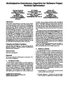
Unfortunately it is not possible to generate meaningful statistics or quality metrics in this paper, because there are no published results with which to make statistical comparisons. Neither are there any known optimum solutions. One contribution of this author is a mechanism for producing lower bounds on the passenger cost, Cp , and operator cost, Co (see supplementary material, [9]). Looking at the results, however, the lower bounds for passenger costs would seem to be better than those computed for operator costs, although the divergence of the best operator costs away from the lower bounds could just as easily be explained by a lack of exploration of the necessary part of the Pareto space. Co Sum of Route Lengths (mins)
y coordinate
25
30
35
Mandl’s Problem 250
20 Results Files Single Results File
200 150 100 50 10
11
20 15 10 5 0 0
Fig. 6.
5
10
15 20 25 x coordinate
30
35
Co Sum Route Length (mins)
y coordinate
30 25
R ESULTS
12 13 14 15 Cp Average Travel Time (mins) Mumford3
16
7000 20 Results Files Single Results File
6000 5000 4000 3000 2000 31
Transport Networks for our new Data Sets Fig. 7.
32
33 34 35 36 Cp Average Travel Time (mins)
Approximate Pareto Fronts Obtained by SEAMO2.
37
Table III shows the best objectives obtained for passengers (Cp ) and operators (Co ) and the corresponding routes for Mandl’s Problem using sets of 10 replicate runs of the SEAMO2 algorithm. These are compared with results from [8], as explained above. In every case SEAMO2 has obtained better results for the passenger objectives, although the operator objective cannot be improved because 63 is equal to the lower bound for R(L). Table IV shows the best cost for passengers (Cp ) and operators (Co ) extracted from the 20 replicate runs for each problem instance, along with the computed lower bounds shown in brackets. Notably, the passenger cost values, Cp are much closer to their lower bound values than is the case for the operator costs, Co . Fig. 7 illustrates the approximate Pareto fronts obtained from a single run (*) and extracted from the 20 sets of replicate runs (o) for two of the instances. The solution quality and spread along the Pareto Front appear to be reasonable for a single run, when compared to the non-dominated solutions extracted from all 20 replicate runs. VII.
C ONCLUSIONS
This paper has presented some new sophisticated problemspecific heuristics and genetic operators for the UTRP in a multi-objective evolutionary framework. The approach balances user and operator costs. Excellent results have been obtained using Mandl’s benchmark, beating previously published results for passenger costs and equaling the lower bound for operator costs. Results are also presented for larger instances created by the author. The new instances and results files are all available for download, providing future authors with much needed benchmarks. To ensure comparability of computational routines with other authors, sample route sets obtained by the present evolutionary algorithm are included complete with respective passenger and operator costs. Furthermore, the test data is supplied with (x, y) coordinates so the the networks and route sets can be visualized. Work is currently underway to introduce additional specialist heuristics to seed the population, and this is producing encouraging results, especially for larger instances. In addition, we are collecting real-world data and experimenting with a range of metaheuristics in addition to EAs. R EFERENCES [1]
[2]
[3]
[4]
[5]
A. Ceder and N. H. M. Wilson, “Bus network design,” Transportation Research Part B: Methodological, vol. 20, no. 4, pp. 331–344, August 1986. T. L. Magnanti and R. T. Wong, “Network design and transportation planning: Models and algorithms,” Transportation Science, vol. 18, no. 1, pp. 1–55, 1984. G. Nielsen, “Hitrans best practice guide 2: Public transport planning the networks,” European Union Interreg IIIB (North Sea Region), Tech. Rep., 2005. F. Zhao and A. Gan, “Optimization of transit network to minimize transfers,” Lehman Center for Transportation Research, Florida International University, 605 Suwannee Street, MS 30, Tallahassee FL 32399-0450, Tech. Rep. BD-015-02, December 2003. M. H. Shih MC, “A design methodology for bus transit networks with coordinated operations,” Center for Transportation, The University of Texas at Austin, Austin, Texas 78705-2650, Tech. Rep. SWUTC/94/60016-1, August 1994.
[6] S. A. Bagloee and A. A. Ceder, “Transit-network design methodology for actual-size road networks,” Transportation Research Part B: Methodological, vol. 45, no. 10, pp. 1787 – 1804, 2011. [7] L. Fan and C. Mumford, “A metaheuristic approach to the urban transit routing problem,” Journal of Heuristics, vol. 16, pp. 353–372, 2010. [8] L. Fan, C. L. Mumford, and D. Evans, “A simple multi-objective optimization algorithm for the urban transit routing problem,” in Proceedings of the Eleventh conference on Congress on Evolutionary Computation, ser. CEC’09, 2009, pp. 1–7. [9] C. L. Mumford, “Data and results,” 2013, the data, results and supplimentary material can be downloaded from: http://users.cs.cf.ac.uk/C.L.Mumford/Research%20Topics/UTRP/CEC2013Supp/. [10] W. Lampkin and P. D. Saalmans, “The design of routes, service frequencies, and schedules for a municipal bus undertaking: A case study,” Journal of the Operational Research Society, vol. 18, pp. 375– 397, Dec. 1967. [11] L. Silman, Z. Barzily, and U. Passy, “Planning the route system for urban buses,” Computers & Operations Research, vol. 1, no. 2, pp. 201 – 211, 1974. [12] C. E. Mandl, “Evaluation and optimization of urban public transportation networks,” European Journal of Operational Research, vol. 5, no. 6, pp. 396 – 404, 1980. [13] ——, Applied network optimization. Academic Press, London ; New York :, 1979. [14] M. H. Baaj and H. S. Mahmassani, “Hybrid route generation heuristic algorithm for the design of transit networks,” Transportation Research Part C: Emerging Technologies, vol. 3, no. 1, pp. 31 – 50, 1995. [15] J. Agrawal and T. V. Mathew, “Transit route network design using parallel genetic algorithm,” Journal of Computing in Civil Engineering, vol. 18, no. 3, pp. 248 – 256, 2004. [16] P. Chakroborty and T. Wivedi, “Optimal route network design for transit systems using genetic algorithms,” Engineering Optimization, vol. 34, no. 1, pp. 83–100, 2002. [17] P. Chakroborty, “Genetic algorithms for optimal urban transit network design,” Computer-Aided Civil and Infrastructure Engineering, vol. 18, no. 3, pp. 184–200, 2003. [18] S. B. Pattnaik, S. Mohan, and V. M. Tom, “Urban bus transit route network design using genetic algorithm,” Journal of Transportation Engineering, vol. 124, pp. 368–375, July/August 1998. [19] V. M. Tom and S. Mohan, “Transit route network design using frequency coded genetic algorithm,” Journal of Transportation Engineering, vol. 129, pp. 186–195, March/April 2003. [20] W. Fan and Y. B. Machemehl, “A tabu search based heuristic method for the transit route network design problem,” in In 9th International Conference on Computer Aided Scheduling of Public Transport, 2004. [21] ——, “Using a simulated annealing algorithm to solve the transit route network design problem,” Journal of Transportation Engineering, vol. 132, no. 2, pp. 122–132, 2006. [22] C. Mumford, “Simple population replacement strategies for a steadystate multi-objective evolutionary algorithm,” in Genetic and Evolutionary Computation (GECCO) 2004, ser. Lecture Notes in Computer Science, K. Deb, Ed. Springer Berlin / Heidelberg, 2004, vol. 3102, pp. 1389–1400. [23] C. Valenzuela, “A simple evolutionary algorithm for multi-objective optimization (seamo),” in Evolutionary Computation, 2002. CEC ’02. Proceedings of the 2002 Congress on, vol. 1, may 2002, pp. 717 –722. [24] G. Colombo and C. Mumford, “Comparing algorithms, representations and operators for the multi-objective knapsack problem,” in Evolutionary Computation, 2005. The 2005 IEEE Congress on, vol. 2, sept. 2005, pp. 1268 – 1275 Vol. 2. [25] I. Harris, C. L. Mumford, and M. M. Naim, “An evolutionary biobjective approach to the capacitated facility location problem with cost and co2 emissions,” in Proceedings of the 13th annual conference on Genetic and evolutionary computation, ser. GECCO ’11. New York, NY, USA: ACM, 2011, pp. 697–704. [26] R. W. Floyd, “Algorithm 97: Shortest path,” Commun. ACM, vol. 5, pp. 345–, June 1962.
TABLE II. Instance Mandl Mumford0 Mumford1 Mumford2 Mumford3
TABLE III.
Nodes and Links Transport net. 15 & 20 30 & 90 70 & 210 110 & 385 127 & 425
Nodes /Route 2-8 2-15 10 - 30 10 - 22 12 - 25
O UR DATA S ETS Nodes in typical Transit net. 6 ∗ (2 + 8)/2 = 30 102 300 896 1110
LBpass (mins) 10.0058 13.0121 19.2695 22.1689 24.7453
LBop = Minimum R(L) (mins) 63 94 294 749 928
ROUTES AND BEST PARAMETERS FOR PASSENGERS AND OPERATOR OBTAINED FOR M ANDL’ S P ROBLEM USING THE SEAMO2 ALGORITHM , COMPARED TO [8] IN BRACKETS . Number of Routes 4
Best Routes for Passengers 1-2-3-6-8-10-11-13 9-15-6-4-12-11-13-14 14-10-7-15-6-4-2-1 12-11-10-8-6-4-5-2
6
1-2-3-6-15-7-10-11 12-11-13-14-10-7-15-9 1-2-5-4-6-8-10-11 1-2-3-6-8-10-13-11 1-2-4-12-11-10-14-13 1-2-5-4-6-8-15-7 1-2-5-4-12-11-10-13 9-15-7-10-14-13-11-12 3-2-5-4-6-8-10-14 8-10-11-12-4-2-3-6 1-2-3-6-8-10-11-13 14-10-7-15-6-3-2-1 10-7-15-8-6-4-2-1 1-2-3-6-15-7-10-13 9-15-8-6-3-2-5-4 15-7-10-14-13-11-12-4 1-2-4-6-8-15-7-10 13-11-10-8-6-3-2-1 1-2-5-4-12-11-13-14 11-13-14-10-8-6-4-5 9-15-7-10-11-12-4-5
7
8
TABLE IV.
Number of Routes 6 12 15 56 60
Parameters for Passenger Routes Cp = 10.57 (10.65) Co = 149 (126) d0 = 90.43 (90.88) d1 = 9.57 (8.35) d2 = 0.00 (0.77) dun = 0.00 (0.00) Cp = 10.27 (10.46) Co = 221 (148) d0 = 95.38 (93.19) d1 = 4.56 (6.23) d2 = 0.06 (0.58) dun = 0.00 (0.00) Cp = 10.22 (10.44) Co = 264 (166) d0 = 96.47 (92.55) d1 = 3.34 (6.68) d2 = 0.19 (0.77) dun = 0.00 (0.00) Cp = 10.17 (10.45) Co =291 (245) d0 = 97.56 (91.33) d1 = 2.31(8.67) d2 = 0.13 (0.00) dun = 0.00 (0.00)
Best Routes for Operators 9-15 1-2-4-5 11-10-7-15-8-6-3-2 14-13-11-12
10-11-13 1-2-3-6-8-15-7-10 5-4-2 14-13 12-11 9-15 12-11-13 14-13 5-4 11-10 10-7-15-8-6-3-2-1 4-2 9-15 12-11 5-4 13-14 9-15 1-2 11-13 2-4 11-10-7-15-8-6-3-2
Parameters for Operator Routes Cp = 13.88 (13.88) Co = 63 (63) d0 = 61.08 (61.08) d1 = 36.61 (36.61) d2 = 2.31 (2.31) dun = 0.00 (0.00) Cp = 13.48 (13.34) Co = 63 (63) d0 = 70.91 (66.09) d1 = 25.50 (30.38) d2 = 2.95 (3.53) dun = 0.64 (0.00) Cp = 14.25 (13.54) Co = 63 (63) d0 = 65.13 (65.64) d1 = 22.93 (26.20) d2 = 10.34 (8.16) dun = 1.61 (0.00) Cp = 14.45 (13.57) Co = 63 (63) d0 = 57.93 (59.92) d1 = 31.92 (21.97) d2 = 9.70 (18.11) dun = 0.45 (0.00)
B EST COSTS FOR PASSENGERS (Cp ) AND OPERATORS (Co ) EXTRACTED FROM THE 20 REPLICATE RUNS FOR EACH PROBLEM INSTANCE . L OWER BOUNDS ARE INCLUDED IN BRACKETS . Best for passenger
Best for operator
Cp CO d0 d1 d2 dun Cp CO d0 d1 d2 dun
Mandl 10.33(10.01) 224 94.54 5.14 0.32 0.00 15.13 63(63) 59.34 30.57 9.06 1.03
Mumford0 16.05(13.01) 759 63.20 35.82 0.98 0.00 32.40 111(94) 18.42 23.40 20.78 37.40
Mumford1 24.79(19.27) 2038 36.60 52.42 10.71 0.26 34.69 568(294) 16.35 29.06 29.93 24.66
Mumford2 28.65(22.17) 5632 30.92 51.29 16.36 1.44 36.54 2244(749) 13.76 27.69 29.53 29.02
Mumford3 31.44(24.75) 6665 27.46 50.97 18.76 2.81 36.92 2830(928) 16.71 33.69 29.18 20.42