New Mathematical and Algorithmic Schemes for Pattern Classification with Application to the Identification of Writers of Important Ancient Documents D. Arabadjis 1, F. Giannopoulos 1, C. Papaodysseus 1, S. Zannos1, P. Rousopoulos 2, M. Panagopoulos 3 and C. Blackwell4 1. National Technical University of Athens, Department of Electrical and Computer Engineering, 9 Heroon Polytechneiou, GR-15773, Athens, GREECE. 2. Technical Institute of Chalkida, Department of Automatic Control, Chalkida, Euboea, GREECE. 3. Ionian University, Department of Audio & Visual Arts, Corfu, GREECE. 4. Furman University, Department of Classics, Greenville, South Carolina, U.S.A.
Corresponding author: Constantin Papaodysseus1,
[email protected], tel. (+30) 210 772 1476, (+30) 210 361 7438 Abstract In this paper, a novel approach is introduced for classifying curves into proper families, according to their similarity. First, a mathematical quantity we call plane curvature is introduced and a number of propositions are stated and proved. Proper similarity measures of two curves are introduced and a subsequent statistical analysis is applied. First, the efficiency of the curve fitting process has been tested on 2 shapes datasets of reference. Next, the methodology has been applied to the very important problem of classifying 23 Byzantine codices and 46 Ancient inscriptions to their writers, thus achieving correct dating of their content. The inscriptions have been attributed to ten individual hands and the Byzantine codices to four writers. Keywords: pattern classification; writer identification; plane curvature; curve fitting; dating ancient inscriptions; dating Byzantine codices; contours similarity
1.
Introduction
1.1
The importance of identifying the writer of ancient inscriptions and Byzantine
codices The set of surviving handwritten documents is one of the main sources for the science of History. More specifically, carved in stone, ancient inscriptions are the most important means of studying Antiquity. Similarly, manuscripts written on both papyri and parchments contributed to the transmission of the ancient world’s literature through the Middle Ages, finally leading to the Renaissance and the Enlightenment. For example, the Homeric Iliad survives mainly through a handful of large manuscript volumes, all produced in Constantinople during the 10th or 11th century and currently scattered in different libraries throughout Europe: Venice, El Escorial in Spain, London, Geneva, Florence and Rome. These volumes contain the Homer’s poem itself, as well as a number of different commentary texts and short notes in the margins of the manuscript and between lines. As one can easily assume from the above, dating of the content of these inscriptions and manuscripts is of particularly high significance for both disciplines of History and Archaeology. “Proper historical use of inscriptions can only be made if they can be dated”, as stated by one of the most influential historians, Prof. Christian Habicht. However, the writers of ancient inscriptions and manuscripts rarely signed or dated their documents, making the process of dating them really difficult; this fact often causes disputes and disagreements among scientists. One major goal of the present paper is to quantitatively analyze the content of a given set of ancient inscriptions and Byzantine codices, so as to determine their relative dates of production, as well as the relationship among them. In fact, carving inscriptions was a profession in Antiquity. The working careers of most ancient writers covered about 20 to 25 years, while very few worked for 40 years, at most. If one achieves in attributing the ancient inscriptions to their writer, then evidently, one has also successfully dated their content. Similar arguments hold for Byzantine codices, which as a rule, were reproduced by monks of the era.
1.2
The goal of the present work
The present paper tries to tackle three problems: 1) To develop and present a new method for optimally matching two curves, one of which may be subject to two independent scaling transformations (along either x or y-axis), rotation and parallel translation. 2) To introduce proper, novel statistical criteria, in order to classify a given ensemble of such curves into proper families/clusters, according to their similarity, based on introduced, new similarity measures. 3) To classify a set of important ancient inscriptions and byzantine codices to the proper writer, so that these documents can be unambiguously dated. There is an underlying fundamental assumption in the proposed solution of the aforementioned problems, which we will elucidate in the case of writer identification: We assume that when a specific writer generates a realization of an alphabet symbol on a document, then the writer may alter the orientation, position and size of the produced letter, rather arbitrarily; however, still, there is a kernel in the generated realization, which remains invariant under the aforementioned transformations and, in addition, is peculiar to the writer himself. Evidently, this, also, may hold true in relation to many other procedures/human activities, as for example in pottery, in painting and arts in general, in contour distortion by noise, etc.
1.3
A brief state of the art in matching and grouping planar shapes Shapes comparison in [1] is treated as a features matching over orientation and
geometric characteristics evaluated by differential properties of the implicit shape’s function. Then, grouping of shapes is performed in a decision trees – based hierarchical clustering context. A features vector – based shape categorization approach is formulated in [2], in a statistical manner. The features of shapes that form a group are mapped on the linear base of their Gaussian graded – mean covariance matrix, which is selected to be the shapes group representative. Registration of planar shapes under affine transformations is studied in [3] using signed Euclidean distance implicit representations of planar shapes. The matching problem is then formulated via the maximization of the mutual information metric in the space of the parameters of affine transformation; maximization is achieved via a steepest descent method. Orientation invariant comparison of planar shapes is treated in [4] in terms of a “proper”
comparison between the sequences of their curvature values. Propriety of the comparison is determined as the re-parameterization of the curves that mostly benefits curvatures correspondence, optimized over all possible differential point-to-point correspondences, using Dijkstra’s algorithm. The approach introduced in [5] concerns N-dimensional curve registration and comparison by evaluating the alignment of the tangential directions of a curve to another fixed curve’s tangents in the conjugate gradient context. In [6] comparison of (closed) planar shapes is based on prototyping shapes deviations as if they were caused by a Newtonian vector flow acting in the interior of each shape. Then, one-to-one shape correspondence is determined as geodesic paths minimizing deformation strains. In [7] and [8], deformation vector flow is modeled as an infinite dimensional (Hilbert) manifold over 1D functions descriptive of closed curves modulo scaling and modulo rotation (in [7]). Then, the curves fitting error is selected so as to retain the inner product defined on the manifold of the integral constraints; this allows for projection and translation of the functional representation of the shapes along paths that minimize the chosen error. A similar formulation that overcomes the infinite expansion of the manifold’s directions is given in [9], where the 2D orthogonal expansion of the shapes’ functional representation is guaranteed by embedding directional vectors in the complex plain. Then, a mapping is constructed, so as to convert the selected metric space into a Euclidean one and thus to “linearize” the problem of geodesics. Authors of [10] extend the representation of a shape in the form of a linear combination of 1D functions to the 2D case, using DC functions (i.e. the difference of 2 convex functions). This is achieved by solving a corresponding L1 optimization problem, modulo uniform scaling and Euclidean transformations.
1.4
A brief state of the art in automatic writer identification Recently, there has been a considerable interest in research on the topics of automated
writer identification and verification, mainly concerning hand written text. Thus, various approaches have been developed, like the [11, 12, 13, 14, 15], based on feature extraction, while Hidden Markov Models are applied to [16, 17, 18]. A lot of research is also being undertaken in association with morphological approaches [19] or texture identification [20]. In [21] a Fourier
Transform approach of the pen-point movement barycenter’s velocity is proposed and in [22] a dichotomy transformation is performed. [23] measures the individuality of handwritten characters through a number of identification and verification models, whereas connectedcomponent contours and allograph prototype methods are described in [24, 25]. More recently, researchers in [26, 27] use a continuous character prototype distribution approach with fuzzy cmeans algorithm in order to estimate the probability that a character has been generated by a prototype. Other scholars [28, 29] tackle the same problem by using a combination of local descriptors and learning techniques or by using directional morphological features [30]. Furthermore, others associate biometric and personal features with the handwriting style [31, 32, 33], while, in [34] certain characteristics of graphological type, such as skew, slant, pressure, thinning area, etc. are employed in order to classify calligraphic handwritten scripts according to their writer. Most recently, methods of automatic writer identification have been applied to text that consists of non – Latin symbols [35, 36], as well as to documents of historical importance [37, 38, 39].
2.
A number of fundamental definitions A first major goal of the present work is to achieve optimal fit for an ensemble of
curves. Towards this direction, we will first define a new quantity we call "plane curvature". In practice, all considered curves will be digital and will lie in a digital image; nevertheless, the strict approach will refer to continuous curves and, next, the algorithmic will consider finite affine and spatial steps. As it will become evident from Sect. 5.1 and the explicit form of the algorithm presented in Sect. 5, optimality of the continuous approach will ensure natural similarity of the involved digitized shapes. DEFINITION 1: Consider a continuous, smooth Jordan curve Γ1 embedded in a sub-domain I of
, where I plays the role of the image frame to-be-digitalized. Let ( x, y ) be the coordinate
system of the sub-domain I. Then, we define an implicit representation of Γ1 as a zero isocontour of a twice differentiable function F ( x, y ) : I R , i.e. F ( x, y ) 0 on Γ1.
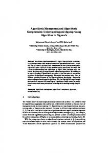
Fig. 1 Depiction of the isocontours of the Euclidean distance from the contour of an alphabet symbol “omega”. This
letter contour, equivalently the zero-level isocontour, is shown in red. DEFINITION 2: Let E be an arbitrary equilevel curve (or isocontour) of F ( x, y ) 0 , i.e. the locus of points ( x, y ) I such that F ( x, y ) c , c an arbitrary constant (see figure 1) and let M be an arbitrary point of E.
Moreover, let n be the unit vector normal to E at M, such that n
F . Then, we define the | F |
function
C( x, y ) n div (n )
(2.1)
is the gradient operator. We will use the term "plane curvature of F" j x y
where, i
for function C ( x, y ) . Since, curve Γ1 is an isocontour of F ( x, y ) , with c 0 , C ( x, y ) on Γ1 is the actual standard curvature of Γ1 at each point of it. Now, suppose that a second smooth Jordan curve Γ2 is also embedded in I and let be the sub-domain of I included between Γ1 and Γ2 (see figure 2a). Then, we may express the similarity of curves Γ1 and Γ2 by means of the "plane curvature error function"
C | n | d
(2.2)
namely, the double integral of the norm of div (n ) on (see figure 2b). Clearly, if curves Γ1 and Γ2 are identical and optimally fit, then C 0 ; if Γ2 manifests deviations from Γ1 and, still, the two curves are optimally fit, then C grows according to the degree of the deviations, as we will show in Sect. 5.1. In other words, the error function defined in (2.2) is strongly connected with a natural interpretation of the variation and similarity between Γ1 and Γ2. In the following, we will prove that if Γ2 is subject to a proper set of transformations, i.e. suitable scaling, rotation and parallel displacement, then curves Γ1 and Γ2 can be optimally matched by minimization of
C.
(A)
(B)
Fig. 2 The sub-domain Ω of discrepancy of the two curves of interest and the plane curvature error function. A) The sub-domain Ω as formed by the discrepancy of the contours of two “omega” symbol realizations. The contour of reference Γ1 is depicted in blue, whereas the transformed one Γ2 is shown in green. Path Γ1 → Γ2 defines the orientation of the boundary of Ω as depicted in the figure. B) Plane curvature error function values in the sub-domain Ω shown in gray-scale; the lower the error value, the darker is the shade.
3.
A number of propositions concerning plane curvature We may consider C as a functional, in the sense that each curve Γ2 embedded in I
generates a different value of C . Therefore, this functional may become minimum for a certain position of curve Γ2, with respect to the fixed curve Γ1; for this position the value of stationery and, hence, ( C ) 0 , namely, the variation of C will be zero. PROPOSITION 1: Error functional C is minimum if the following error functional
will be
C ( n ) 2 d
(3.1)
is, also, minimum in the same position of curve Γ2. Equivalently, ( C ) 0 ( C ) 0 . Hence, the following holds PROPOSITION 2: Minimization of error C is equivalently expressed by means of minimization of the following error function:
C 2 n dl
(3.2)
2
PROOF We will demonstrate the proposition by minimizing the functional
. In fact, by applying
Stokes Theorem, we obtain:
( n )
2
d ( n )( n )d ( n ) n ˆ dr n (( n ))d
(3.3)
where, is the boundary of the domain and ˆ its unit normal vector. But,
is the directional derivative
( n ) along the unit vector n . In addition, if n
l is the unit vector tangent to Γ2 at an arbitrary point of it, dl the elementary arclength of Γ2
and
the elementary length normal to l towards Γ1, then d dn dl ; the reason for the
minus sign is that we want curve Γ2 to "move" towards Γ1, opposite to the unit vector normal to
of Stokes theorem. ( n ) ( n ) Then, n (( n ))d d dndl n dl n n Therefore, substituting in (3.3) we obtain:
2
C 2 n dl C 2 n dl n dl
1
(3.4)
Functional C remains always greater than or equal to zero, hence, it has a minimum for a certain position of Γ2 at which it holds ( C ) 0 . But, since curve Γ1 is kept fixed, it follows that (
1
n dl ) 0 . Hence, ( C ) 0 ( n dl ) 0 2
Taking into consideration proposition 1, too, it follows that ( C ) 0 (
2
n dl ) 0 Q.E.D.
PROPOSITION 3: Let ( x, y ) be an arbitrary point of I, Ε be the isocontour of F ( x, y )
passing from it and n n x i n y j be the unit normal vector defined in Section 2.
x Passing in matrix notation, let ∇ be the gradient matrix, H x x y y
2 x 2 2 xy
y
2 yx be the matrix of the Hessian operator. 2 y 2
F Then 2 x
F 2 2 F x F F y F x y y
0
(3.5)
1
is the norm of F ; moreover, let J be an auxiliary matrix. Then, the plane 1 0 curvature at point ( x, y ) is also expressed via the relation
C ( x, y )
1 F 3 x
F x F T J H J F y y
The proof of Proposition 3 is given in Appendix A
(3.6)
4.
Plane curvature variation under affine transformations To achieve optimal matching between curves Γ2 and Γ1, we apply the following original
approach: We impose scaling, rotation and parallel displacement to the entire domain I and, in particular, to both curves Γ2 and Γ1. In this way, after a set of such transformations, we obtain
~
~
~
the transformed curves 2 and 1 . As a result, the isocontours of 1 also change, thus
changing the value and direction of unit vector n . Hence, plane curvature C ( x, y ) also changes value and the purpose of the present Section is to calculate the precise form of this change. We would like to emphasize that although the entire domain I is subjected to the above affine transformations, nevertheless, the fitting errors C , C , C are computed in the domain
~ and each contour defined by the non-transformed curve Γ1 and the transformed one 2 . Equivalently, we transform the entire domain I, in order to achieve proper affine
~
transformations of Γ2, but the resulting, under these transformations, curve 2 is always compared with the intact curve Γ1 which is supposed to remain fixed over the transformed domain I. The implementation of the approach requires stating and demonstrating the following set of definitions and propositions, associated with the change of I under these transformations. DEFINITION 3: We express the elementary scaling, rotation and parallel displacement imposed to every point of I, by means of the elementary matrix:
0 1 1 da A 1 db dT 0
dT 1 0 da 1 0 1 dT
dT I 2 dA db
(4.1)
where, we consider only first-order calculus and a mono-parametric group of transformations,
I 2 is the 2x2 unit matrix, dA is the elementary part of A, (1 da ) is the scaling factor along x-axis, (1 db) is the scaling factor along y-axis and dT is the elementary angle of rotation
d x
around the understood z-axis. If we also consider the elementary displacement , which d y
we assume it is the same for all points of domain I, then the arbitrary point ( x, y ) I , under the set of these elementary transformations originates to a point ( ~ x, ~ y ) by the relation:
x d x x ~ A y ~ y d y
(4.2)
We should note that ( x, y ) and ( ~ x, ~ y ) are in an one-to-one correspondence, since A is locally invertible with A 1 I 2 dA in a first order approximation. Thus ( ~ x, ~ y ) results from the infinitesimal transformation of ( x, y ) by:
x d x x ~ ( I 2 dA) ~ y d y y LEMMA 1: The gradient operator ∇, under transformation (4.2), changes according to
~ T x A ~ y
x ~ T A y
(4.3)
In addition, the norm of F changes according to
~ T F AA T F
(4.4)
while, the Hessian operator is transformed according to
~ H AT HA
(4.5)
PROPOSITION 4: Under transformations (4.2), the plane curvature changes by dC given by
dC C
F 2 2 x
g a da g b db
2
(4.11)
2
where g a 3
(4.11a)
2
F and g b 3 2 2 y
(4.11b)
PROOF
~ ~ According to proposition 3, the plane curvature C ( ~ x, ~ y coordinates as x , y ) is written in the ~
~ ~ ~ ~~ ~ ~ ~ T F J T HJ F C( x , y ) ~3
(4.12)
Using the results of Lemma 1, (4.12) is written:
~ ~ T F AJ T A T H AJA T F C(~ x, y) (T F AA T F ) 3 2
0
But, AJ T A T (1 da )(1 db)
(4.13)
(1 da )(1 db) (1 da )(1 db)J T 0
(4.14)
Therefore, (4.13) now becomes:
T F J T H J F ~ ~ C(~ x , y ) (1 da ) 2 (1 db) 2 T ( F AA T F ) 3 2 T F J T H J F ~ ~ C(~ x , y ) (1 da ) 2 (1 db) 2 3
~ ~ C(~ x , y ) (1 da ) 2 (1 db) 2
3 (T F AA T F ) 3 2
3 (T F AA T F ) 3 2
C ( x, y )
(4.15)
~
Letting C C dC and using (3.4), we obtain:
(1 da ) 2 (1 db) 2 | F |3 (T F AA T F ) 3 2 dC C (T F AA T F ) 3 2 Now, (T F AA T F ) 3 2
2 2 F 2 F 2 F F ~ ~ 2da ~ 2db ~ x y x y
(4.16)
32
and after using Taylor expansion and keeping first order terms only, we obtain:
(T F AA T F ) 3 2
F 2 F 2 2 da 3 2 db 3 2 2 x y
2
(4.17)
2
F F 2 Evidently, using the definition of g a 3 2 2 as in (4.11), 2 and g b 3 x y 2
the desired result follows immediately.
Q.E.D.
COROLLARY 1: Suppose that we, sequentially, apply a set of transformations of type (4.2), thus obtaining a finite composite transformation, which maps the initial curve 2 to another
~
curve 2 . Let ( x, y ) be an arbitrary point of 2 , which, under this finite composite
~ transformation, moves to point ( ~ x, ~ y ) 2 . It is understood that during this transformation, the pair of scaling factors (a, b) change along a curve Δ in their coordinate system, starting at
~
identity point (1,1). Then, the plane curvature C ( ~ x, ~ y ) is related to C ( x, y ) via formula g da g db ~ ~ a 2 b C(~ x, y) e C ( x, y )
(4.18)
where the line integral in the exponent is computed upon path Δ.
In order to use solution (4.18) to parameterize the affine transformation of the xy - plane by means of a desired curvature deformation, we need to evaluate the sensitivity of the line integral of (4.18) to the variations of path . In other words, we should evaluate the 2nd order variation
~
of ln C ( ~ x, ~ y ) under the infinitesimal transformation (4.1). This evaluation is performed in Appendix D and the obtained results are summarized in the following proposition PROPOSITION 5: Under infinitesimal transformation (4.2), the second order variation of the plane curvature function logarithm ln C ( x, y ) is independent of the absolute size of the path differential (da, db) and depends only on the ratio
da . Namely, for ab and db
1 2
(a 2 b 2 ) it holds that d ln C 0 , a 1 b1
d 2 ln C d 2
0 1 2 1 ln C ~ nT n 2 a 1 1 0 b 1
(4.19)
Hence, according to the aforementioned Proposition 5, the variation of the tangent of the integration path at the origin depends only on the tangent’s direction and not on its measure. Therefore, the determination of the optimal transformation path that minimizes the plane curvature discrepancy between two curves, depends only on the direction of the tangent vector at the transformation’s identity point (starting point of ) and, consequently, it is parameterization invariant. So, this optimization can be performed independently of the
(da, db) - discretization size, making the whole - interpolation procedure uniformly stable and robust. The previous analysis indicates that plane curvature variation, under transformations (4.1), (4.2), depends only on two independent variables and in particular, the scaling factors
(a, b) . However, the optimum placement of two curves 2 and 1 depends on three additional parameters corresponding to the rotation of the curve 2 around the z-axis, as well as on the parallel displacement of 2 along x,y-axes. Since, we have previously established that optimal scaling can be achieved independently of rotation and displacement, by means of the introduced plane curvature approach, then it is logical to expect that there are infinitely many positions of curve 2 , for which the plane curvature error C is minimum; these positions, obviously, correspond to the infinitely many rotations and displacements that may be applied to 2 .
~
Nevertheless, we may adopt the quite standard criterion of actually optimal fit of 2 and 1
~
inside domain , which demands the integral of Euclidean distances of all points of 2 from 1 to be minimum; then, we may employ this criterion together with the previously obtained
~
results, in order to achieve best fit of 2 and 1 inside domain I, when all transformations are taken into consideration. This will be the subject of the next Section.
5.
A new method and the corresponding algorithm for fitting two
curves Γ1 and Γ2 In this Section, we will employ the previously obtained results and we will define a new similarity measure, in order to present the steps of a novel algorithm, which performs best fitting of any two Jordan curves Γ1 and Γ2 inside domain I. This novel approach may be embedded in any function minimization algorithm, such as the Nelder-Mead. The introduced curve fitting method consists of two stages: I) In the first stage, the optimal resize factors a and b are obtained, for which the overall plane curvature difference of Γ1 and the transformed Γ2 is minimum. Evaluating both these resize factors a and b independently is legitimate, since we have already proved in previous Sections that this procedure is independent of rotation and parallel translation. We should note here that determination of the optimal scaling factors a, b through simple normalization of the curves length or of the area they enclose, etc., is legitimate / correct only in the case where the normalized curves coincide. As it will be shown in Sect. 5.1 by minimizing the curvature measure we obtain optimal scaling for an arbitrary pair of curves, independently of Euclidean transformations. II) In the second stage, we first define a proper similarity measure of Γ1 and the optimally resized Γ2 to incorporate rotation and parallel translation. Then, the method may employ any function minimization algorithm, in order to determine the optimal relative match of Γ1 and the transformed Γ2. These stages are described below.
5.1 Connection of the selected curvature measure with natural measures of shapes similarity The implicit curvature measure introduced in Definition 2, Section 2, is strongly connected with the natural interpretation of the possible variations of a shape, i.e. the variations caused by vector field actions respecting a metric. Namely, considering the geodesics with tangents along
vector field n , we can evaluate the deviations from an isocontour Γ1 of F ( x, y ) , inside the
family of curves that F ( x, y ) induces, by the geodesic length ( p1 , p )
F ( p)
0
| dF | , between F
a point p1 1 and an arbitrary point p of the xy – plane. Then, letting p belong to a planar curve 2 , we can evaluate the deviation of 2 from 1 by the Lagrangian integral
D( 1 , 2 ) ( p1 ( s), p)ds , where s [0, ] is the curve length parameterization of 1 . 1
Then, any transformation of the xy – plane with infinitesimal length dt moves ( x, y ) to
( x' , y' ) ( x, y ) dt v , where v is an arbitrary unit vector indicating the direction of the transformation of ( x, y ) . The effect of this transformation on D( 1 , 2 ) is given by the action
of the corresponding vector field v on the integrands of D( 1 , 2 ) . Namely,
D(1 , 2 ) ( p1 ( s), p)ds ( p1 ( s), p) d s( p1 ) 1
Evaluating separately the action of on and ds , we have
d ( [ s]) d (v l )
( p1 ( s), p) (v n )( p) (v n )( p1 ) ,
where l is the unit vector tangent to 1 . Thus, the infinitesimal deviation of D( 1 , 2 ) reads
D( 1 , 2 ) ( p1 ( s), p) v ( p) l ( p1 ) s0 v n pp ( s ) ds d v pp ( s ) l s
1
1
1
But, while moving on 1 we always have ( p1 , p1 ) 0 , implying that d ( p1 , p1 ) 0 . In
addition, moving on paths along n that connect points p1 and p , p1 remains unchanged implying that ds 0 .
s
Thus, ( p1 , p) v ( p) l ( p1 ) s 0
p d v p ( 0) l
1
2
1
p d v p ( ) l
2
1
1
.
So, considering domain defined by the paths connecting points p1 and p for all p1 ( s) 1 ,
s [0, ] , we can evaluate the 1st order variation of D( 1 , 2 ) using Stokes’ theorem in the form
D( 1 , 2 ) v ˆ d v d
(5.1)
Where ˆ is the unit vector normal to , with orientation that respects positive step ds along
1 . Expressing differential displacement dt v of the Cartesian coordinates in the curvilinear
frame ( n , l ) , we obtain dt v nd l ds . Also, it holds that (dt v ) dt v v dt .
Since v is unit vector and dt differential length along v , dt dv and v dv 0 , thus
implying that (dt v ) dt v . Evaluating (d n ) and (ds l ) in the same way, we
obtain dt v d n ds l (ds d ) n v v (l n ) n .
Substituting this expression for v in (5.1), the 1st order variation of D( 1 , 2 ) has norm
D( 1 , 2 ) 2 | n | d
(5.2)
which is the implicit curvature measure of (2.2). Therefore, the introduced implicit shapes similarity measure is the supremum of the Euclidean norm of the 1st order variation of the geodesic length between a pair of shapes, inside a given curves’ family.
5.2 Optimal transforming Γ2 in size, so as to fit Γ1. Matching Γ2 to Γ1, as far as minimum plane curvature error is concerned, comprises the following steps: Step 1: We consider curve Γ2 at its original position inside I and for each point ( x, y ) 2 , we compute quantities g a , g b , via relations (4.11a), (4.11b), (3.5). Step 2: We initially set a=1, b=1 so as to begin from the identity point of the transformation to be computed. Then:
a) We first compute 1
1
n dl ; this integral is numerically computed only once and on
the nearest to Γ1 isocontour, outwards to Γ2, in the digital domain I. b) At each point ( x, y ) of Γ2 we consider the isocontour of F ( x, y ) passing from it, we
compute n and we attribute this value to C ( x, y ) . This ensemble of values C ( x, y ) play the role of the initial values of the plane curvature in curve Γ2 and for this reason, we will, hereafter, employ for it the symbol C02 ( x, y ) . Evidently, subscript 0 indicates that this curvature is computed at position 0, namely the initial one, while superscript Γ2 indicates that this curvature refers to Γ2. We would like to point out that we actually obtain a set of values of
C02 ( x, y ) , where each value is computed at the center of a corresponding pixel of the digitized
version of Γ2. In addition, we emphasize that n for Γ1 is computed on the nearest isocontour
outwards to it; we do so, in order to avoid discontinuities in the value of n , on curve Γ1, due
to the fact that unit vector n changes orientation as we cross the corresponding curve. Step 3: In order to decrease error function | C | under the infinitesimal deformation (4.11), we determine the locally optimal finite steps δa,δb (discretizing da,db), in the frame of a function minimization algorithm, for example the Nelder-Mead. Next, the corresponding change of plane curvature C02 ( x, y ) for all previously defined points in Step 2, is computed via (4.11) to give
dC ( x, y ) C02 ( x, y )
g aa g bb
2
Then, the new plane curvature C12 ( x1 , y1 ) , at point
( x1 , y1 ) obtained from ( x, y ) via resize by factors (1 a,1 b) , is C12 ( x1 , y1 ) C02 ( x, y ) dC ( x, y ) . Performing this update for all appoints of 2 , we reestimate (re-draw) it applying to all ( x, y ) 2 the following transformation, which is actually
x1
1 0
a
(4.1) and (4.2) properly adjusted: y1 0 1 0
0 x We emphasize that in b y
(4.1) and (4.2), we have set the rotation and parallel displacement parameters equal to zero, i.e.
dT d x d y 0 , since, as we have proved in the previous Sections, the change of plane
curvature is independent of rotation and parallel translation. The ensemble of points ( x1 , y1 )
~
forms the transformed version of digital curve 2 , say 2 ( x1 , y1 ) .
~
Step 4: The error functional | C | is computed for the new version 2 ( x1 , y1 ) by means of relation (3.4). In fact, we digitally compute 2
2
n dl by numerically integrating
~ C12 ( x1 , y1 ) on 2 . If | C | is smaller than a properly selected threshold, usually associated with the function minimization algorithm, then the procedure stops. Otherwise, it proceeds to the next Step 5, which is actually Step 1 with different starting values.
~
Step 5: We compute g a , g b , via relations (4.11a), (4.11b), (3.5) on 2 ( x1 , y1 ) . Step 6: We return to Step3 and we repeat the optimal transformation process up to Step 5 for
~ ~ 2 ( x1 , y1 ) , thus obtaining a new transformed version 2 ( x2 , y2 ) of digital curve 2 and so on, until the termination condition in Step 4 is met. Namely, until the error function | C | reaches a minimum.
~
At the end of this process, we obtain the best 2 version of 2 , as far as difference of
~
plane curvature of 2 from 1 is concerned ( | C | is minimum). We should denote here that, in Sect. 4, by means of Proposition 5, it has been shown that the performance of this optimization procedure does not rely on the absolute size of the discretization steps (a, b) ; this size only affects the density of the transformation’s identity points’ selection.
5.3 Incorporating rotation and parallel translation for optimally fitting Γ2 to Γ1.
~
From the moment that the best 2 has been evaluated, one expects that there would be
~
infinitely many different placements of 2 relative to 1 , for which | C | is minimum, since, as we have already shown, minimization of plane curvature difference is independent of rotation and parallel translation. Therefore, the developed matching algorithm must account for these transformations, too. Thus, one may employ any typical error function and integrate it into a
function minimization algorithm. For reasons that will be analytically explained in the following, we have chosen the subsequent, quite standard matching error:
~
Let P be an arbitrary point of 2 and let d (P) be the Euclidean distance of P from 1 .
~
Then, the error of fitting 2 to 1 that has been employed is
~ 2
d ( P )dl , namely, the
~
curvilinear integral of the distance of all points P of 2 from 1 .
~
At each step of the employed function minimization algorithm, the new position of 2 is re-estimated by means of (4.1) and (4.2), after setting da=db=0, since the minimization of the plane curvature difference has already been achieved via the algorithm of Section 5.2. We note
~
that rotation is applied only to 2 and not to the entire shape image I. Eventually, via application of the introduced method, the optimal fit of curves
and
is achieved, where curvature similarity, rotation, x and y parallel translation altogether have been taken into account. A number of results of such a fitting procedure in association with contours of letters appearing on ancient inscriptions and Byzantine codices are displayed in figures 3,4.
(A)
(B)
Fig. 3 Depiction of the matching procedure applied to two letter contours belonging to different codices. A) Initial and optimal placement of two “kappa” symbol contours. The reference, fixed contour is depicted in blue. The initial position of the curve to be matched is shown in red and its optimal transformed version in green. B) Intermediate deformations of the transformed contour towards convergence, are presented by the curves in red. The final curve of this deformation process is rotated and translated, so as to optimally fit the reference one.
(A)
(B)
Fig. 4 Depiction of the matching procedure applied to two letter contours belonging to different inscriptions. A) Initial and optimal placement of two “alpha” symbol contours. The reference, fixed contour is depicted in blue. The initial position of the curve to be matched is shown in red and its optimal transformed version in green. B) Intermediate deformations of the transformed contour towards convergence, are presented by the curves in red. The final curve of this deformation process is rotated and translated, so as to optimally fit the reference one.
5.4 The introduced measures of similarity of two curves.
~
After obtaining the optimal position of 2 and 1 , if one employs the previously defined fitting errors as similarity measures of curves 1 and 2 , then one will meet with serious inconsistencies; we stress that these inconsistencies are associated with the measure of similarity of curves 1 and 2 and not with the best fit of these curves, which is optimally achieved by means of the method introduced in 5.2 and 5.3. In fact, the various alphabet symbols realizations inside the very same manuscript manifest substantial variation in size and curvature distribution of the contour. Therefore, if one matches all realizations of the same alphabet symbol in a manuscript to a specific realization contour 1 , then the obtained errors will immediately depend on the size and mean curvature of the reference letter. In such a case, statistical processing of the obtained error values may be meaningless. Equivalently, in order to apply a consistent statistical decision, like the one that will be introduced in the following Section, one must first define a measure of similarity of 2 and 1 that is as much independent
as possible of the size and mean curvature of the chosen reference curve 1 . For this reason, we
~
have defined and employed the following measures of similarity of 2 and 1 :
DEFINITION 4: a)
Similarity measure in plane curvature space
~
Let | C |M be the obtained minimum value of plane curvature difference between 2 and 1 and consider the already computed 1
1
n dl , namely the integral of the plane curvature
on the nearest to Γ1 isocontour, towards Γ2, in the digital domain I; this integral has already been computed in Step 2 of Section 5.2.
~
Then, we define the similarity measure of 2 and 1 , as far as plane curvature difference is concerned, via relation: | b)
C
|S
| C |M
1
.
Similarity measure in Euclidean space
~
Consider 2 rotated and translated, so as to optimally fit 1 according to the previously defined Euclidean error. If
~2
d ( P )dl is the corresponding minimum fitting error, then the M
d ( P )dl ~ ~ ~2 M similarity measure of 2 and 1 is defined via: M ( 1 , 2 ) ~ ( 1 )( 2 ) ~
~
Where ( 1 ) and ( 2 ) are the lengths of curves 1 and 2 respectively.
~
DEFINITION 5: The overall similarity measure of 1 and 2
~
The overall similarity measure of the two curves 1 and 2 is given by:
~
~
(1 , 2 ) | C |S M (1 , 2 ) ~
Where is a constant, properly chosen to ensure that the two errors | C |S and M ( 1 , 2 ) are of similar order of magnitude.
~
We will plausibly adopt that ( 1 , 2 ) is an implicit measure of the similarity of the two initial curves 1 and 2 ; this claim is fully supported by the analysis and the results
~
introduced in Sect. 5.1. Actually M ( 1 , 2 ) is the geodesic path error, when F ( x, y ) is the Euclidean distance transform, while | C |S is the supremum of the first order variation of this error. The efficiency of the chosen similarity measure will also be justified by the final writer identification results.
6.
Statistical criteria for classifying a given set of shapes into
groups – Application to writer identification 6.1
Determination of the different writers of a given set of documents Let us consider two distinct documents D1 and D2 and a specific alphabet symbol, say
L, N1L realizations of which appear in D1 , while N 2L realizations of it appear in D2 . We arbitrarily choose a first realization of L in D1 , we call it L1,1 and we perform all pair-wise comparisons of it with all other realizations of L on D1 namely L1, 2 , L1,3 ,…, L1, N L . In 1
order to perform these comparisons, we embed L1,1 and L1,i in the same domain I, which may be thought of as a rectangular white digital image. We apply to this couple of curves the method introduced in Sections 2, 3, 4, 5 and, thus, we obtain a similarity measure of the type described
~
in Section 5.4, which we denote ( L1,1 , L1,i ) . Subsequently, we consider realization L1, 2 as the reference one and we compare it with L1,3 , L1, 4 ,…, L1, N L , by means of the introduced method, 1
~
thus, obtaining a set of similarity measures ( L1, 2 , L1,i ) , i > 2 and so forth, until L1, N L 1 is 1
compared with L1, N L . Associated optimal fitting positions of pairs of contours of various 1
alphabet symbols realizations are shown in figures 3a, 4a.
We assume that the obtained
( N1L 1) N1L ~ similarity measures ( L1, j , L1,i ) , i > j come from a 2
normal distribution; the performed Kolmogorov-Smirnov test did not violate this assumption (a=0.01) as well as the related simulation experiments (see figure 5). We let 1 be their mean
~
value of ( L1, j , L1,i ) and S1 be their standard deviation.
Fig. 5 : Histogram of the similarity measure, shown in blue, together with the theoretical normal distribution optimally fit to it, shown in red.
As a next step, we apply the method to all pairs of realizations L1,i , i 1,2,..., N1L and
~ L2, j , j 1,2,..., N 2L and we obtain another set of values ( L1,i , L2, j ) , i 1,2,..., N1L ,
~ j 1,2,..., N 2L . We again assume that the obtained N1L N 2L values ( L1,i , L2, j ) come from a normal distribution; the performed Kolmogorov-Smirnov test did not violate this assumption (a=0.01) as well as the related simulation experiments. We let 2 be their mean value of
~
( L1,i , L2, j ) and S2 be their standard deviation. Then, if 1 , 2 are the (unknown) theoretical means of the two normal populations and if N1L,1
( N1L 1) N1L L L L and N1,2 N1 N 2 , it is well known that quantity 2
tL
(1 2 ) ( 1 2 ) (S1 ) 2 (S2 ) 2 N1L,1 N1L, 2
(6.1)
follows a Student distribution with d degrees of freedom, where d is the integral part of 2
(S1 ) 2 (S2 ) 2 NL NL 1, 2 1,1 2 2 (S1 ) 2 (S2 ) 2 L NL 1,1 N1, 2 N1L,1 1 N1L, 2 1
(6.2)
As it has already been noted, the population theoretical means 1 , 2 are, as a rule, not known; nevertheless, if one makes the hypothesis that the two documents D1 and D2 have been written by the same hand, then, a priori, 1 2 . In this way, quantity t L in (6.1) has a well-defined value and therefore, the validity of the hypothesis H0, where H 0 : 1 2 , can be tested against the complementary hypothesis H 1 : 1 2 . The degree of confidence with which these hypotheses will be tested is chosen by heuristic arguments. Indeed, in practice, since inscribing stones was a profession up to the Hellenistic Period, one may safely consider that the ensemble of all unearthed inscriptions so far, were inscribed by a maximum of few hundreds of writers. At the same time, one may expect that a quite complete database of these inscriptions should include some tenths of thousands of them. Thus, since multiple comparisons will be performed, as it will be described below, if we also take the Bonferoni approach [40] into consideration, a logical value for the threshold of the level of significance a is aT
10 4 , where ‘n’ is the number of the performed statistical tests n
associated with the number of different alphabet symbols, on which the introduced methodology is each time applied. Given that analogous arguments hold for the Byzantine codices too, the same a T value can be used as a threshold, also for the considered codices. Therefore, if
P( x | t L | | t L | x ) aT , then H 0 is rejected and H 1 is adopted; otherwise, one cannot reject H 0 , with a considerable confidence. Next, we proceed as follows in order to take into account the entire set of considered documents 0 {D1 , D2 ,..., D } : we apply the introduced methodology to each pair of documents ( D1 , D p ) , p 2,..., for all alphabet symbols L appearing in the entire set of documents. We repeat the same procedure, employing now document D2 , as a reference one. Then,
D3 , subsequently D4 and so forth, until document D 1 is compared with D for all selected, common to all documents, alphabet symbols L. For every pair of documents, for which H 0 is rejected and for each comparison between L appearing in them, we keep the one with minimum
P - x - t L t L x , provided that this probability is smaller than aT ; let this pair
of inscriptions be Dq1 , Dq2 . Then, reasonably enough, we assume that Dq1 and Dq2 have been written by two different hands, say W1 and W2 . We let document Dq1 be the first document associated with writer W1 and actually, we assume that this document is a first good representative of its writing style and for this reason, we denote Dq1 with the alternative symbol
1 . Similarly, we let Dq 2 be the first good representative of the writing style of W2 and for this reason, we denote it with the alternative symbol 2 . Subsequently, we remove documents Dq1 and Dq2 from the ensemble of the considered documents 0 , thus, reducing the ensemble of the manuscripts to-be-classified to
1 0 {Dq1 , Dq2 } . At this point, we take into consideration all pair-wise comparisons of each unclassified document of set 1 with manuscripts 1 and 2 , equivalently with documents Dq1 , Dq2 . In fact, consider an arbitrary Di 1 and let it be matched with 1 first
and 2 next, by means of the introduced methodology. In this way, for each alphabet symbol L L L separately, two similarity measures, two corresponding values ti ,1 , ti , 2 (via 6.1) and two
L L corresponding tail probabilities Pi,1 - x - t i,1 t i,1 x and
L L Pi,2 - x - t i,2 t i,2 x are obtained. We choose the maximum of Pi,1 and Pi,2 and
then the minimum of all these maxima for all alphabet symbols L appearing in the compared documents, i.e. αi min over all L {max{ Pi ,1 , Pi , 2 }}. Now, we consider all α i with value smaller than the threshold of the level of significance α Τ , i.e. all αi α Τ and we choose the minimum of these α i that corresponds, say, to manuscript Dq3 . Then, we assume that Dq3 belongs to a third writer, denoted by W3 , adopting that Dq3 is a good representative of the writing style of W3 ; for this reason, we resymbolize Dq3 as 3 . In other words, in case that there is at least one alphabet symbol in Dq3 , whose realizations are drastically different from the realizations of this symbol on both 1 and
2 , then we decide that document Dq3 belongs to a different writer, with a considerable confidence. Proceeding in an analogous manner, we remove document Dq3 from 1 , thus obtaining the set 2 1 {Dq3 } 0 {Dq1 , Dq2 , Dq3 } . We take into consideration the results of all pair-wise comparisons between each document of 2 with 1 , 2 , 3 , in connection with all alphabet symbols L appearing in the compared documents. In this way, we obtain
α i min max{ Pi ,1 , Pi ,2 , Pi ,3} over all L
and we spot the minimum of α i , provided that αi α Τ , if any. Consequently, we spot a new writer W4 , with 4 being a good representative document of his writing style. We continue the process until inequality αi α Τ is not satisfied for any comparison whatsoever. In this case, we end up with a number of writers (different hands) W1 ,W2 ,...,W
and their corresponding representative documents 1 , 2 ,..., . We would like to stress that, on the considered application, the determination of different hands is quite independent of the choice of the α T value, the only restriction being that the order of magnitude of α T is reasonable. In other words, when the number of distinct hands has been reached, then an important “jump” in the order of α i is observed; thus, the group of the representative documents 1 , 2 ,..., can quite safely be distinguished. In practice, at the end of this process, there will be a set of unclassified documents
U 0 {Dq1 , Dq2 ,..., Dq } ; therefore, it is necessary to develop a method for classifying the documents of U to the proper writer W1 or W2 or…or W .
6.2
Classification of the remaining documents to the proper writer Let us consider any document Di U ; we compare Di with each one of
1 , 2 ,..., by means of the introduced method. More specifically, consider Di and document 1 and suppose that there are realizations of alphabet symbol ‘A’ appearing on both these documents. Then, we momentarily assume that Di and 1 have been written by the same hand, in which case, the theoretical population means 1 and 2 in (6.1) are equal. Under this A assumption, the value of ti ,1 is known and, consequently, the value of the underlying Student
distribution at this point, f
St
t is known. We repeat this procedure for alphabet symbols A i ,1
appearing both in Di and 1 ; let i ,1 be the number of these common alphabet symbols denoted by G1 , G2 , Gi ,1 ; in the previous examples G1 ' ' , G2 ' ' , etc. Then, we define the likelihood of similarity of documents Di and 1 , as far as the writing style is concerned, by means of
i ,1
i ,1
i ,1
f p 1
St
(tiGp ,1 )
(6.3)
This is so, because if Di and 1 have been written by the same hand, then it is unlikely that
tiGp ,1 will be far away from the y-axis. On the contrary, it is logical to assume that if they have Gp not been written by the same hand, then ti ,1 would have a particularly small value for at least a
number of common alphabet symbols G p . We employ the root of order i ,1 to ensure that the order of the likelihood i ,1 is independent of the number of the common symbols between Di and 1 . We repeat this process for all pairs of compared documents Di and j , thus obtaining a corresponding likelihood value i, j . We compute the maximum of i, j overall j and say that this maximum occurs at j = q; namely, comparison of document Di with representative document q offered the maximum likelihood i,q . In this way, we attribute document Di to writer Wq who has q as his representative document. Next, we remove Di from U and we repeat the aforementioned process until no more unclassified documents remain. 6.3
Classifying a given set of curves according to an arbitrary property 𝒫. The previous analysis presented in sub-Sections 6.1 and 6.2 refers to the classification
of alphabet symbols according to their writer. However, this approach may be directly generalized, so as to tackle the problem of classifying an ensemble of arbitrary shapes according to a property 𝒫, having the following characteristics: property 𝒫 divides the ensemble of given curves into distinct families; if a member of each such family is subdue to rotation, parallel translation or resize along the x and y-axis separately, then the corresponding curve remains inside the very same family. The introduced method does not require any database of reference shapes or any a priori knowledge, except of a plausible choice of the threshold a T of the level of significance. In other words, given an ensemble of curves, which do not necessarily represent letters, in order to optimally match any two of them, we first apply the plane curvature methodology introduced in Sections 2, 3, 4 and 5.2, thus obtaining the optimal resize factors a and b.
Afterwards, we apply rotation and parallel translation to the already resized curve and we optimally place the two compared curves, so as the corresponding error, as described in Section 5, is minimum. Then, we spot the statistical distribution of similarity measure ; if property 𝒫 is multi-parametric, then we assume that follows a normal distribution due to the Central Limit Theorem. In any case, one may test the theoretical assumption about the statistical distribution by employing the Kolmogorov-Smirnoff test. As a next step, we apply proper statistical tests to determine the number of distinct families of curves according to property 𝒫. At this point, selection of a plausible value for the threshold
of the level of significance is crucial and depends on a certain “high level”
knowledge of property 𝒫. This process will attribute to each family of curves a representative curve corresponding to the minimum two-tailed area of the performed statistical comparisons or equivalently the curve that differs most from the others, statistically. Finally, unclassified curves are attributed to the proper family by means of a maximum likelihood approach employing a likelihood measure of the type of (6.3); evidently, the underlying probability density functions will correspond to characteristics of property 𝒫, but they will always be those of the type of (6.1) with degrees of freedom analogous to (6.2), when
follows a normal distribution. 6.4
Time complexity of the whole curves’ classification system Concerning the time complexity of the classification methodology, described in Sects.
6.1 and 6.2, we should note that the whole system mainly splits into 2 sub-procedures : A) First, optimal affine registration is performed for all pairs of curves and the fitting error of each pair is computed and stored. B) Next, using all pair-wise fitting error results, the probabilistic classification procedure of Sects. 6.1 and 6.2 sequentially classifies the considered curves into groups. Evidently, the first procedure is parallelizable by simple distribution of the data in a 2D processors grid and requires minimal message passing (i.e. just to read the distributed data and to publish the results when execution ends). Concerning the classification procedure, we note that it is sequential and thus, it cannot be parallelized. However, the likelihood calculations are
performed pretty rapidly and the corresponding execution time is by no means comparable to the execution time of the first procedure. Actually, implementing the methodology using C in a computer with a processor of 2 cores, each clocked at 2.8 GHz and with 6MB L2 cache, the first procedure returned all pair wise comparisons of the instances of an alphabet symbol in any 2 documents in less than 10 sec. Moreover, execution time of the statistical classification procedure in both writer identification applications did not exceed 0.5 sec. Evidently, the smaller the documents, the faster the execution time; in certain cases, this procedure lasted for less than a second. We once more state that we have applied the introduced methodology in 46 inscriptions and 23 byzantine codices. The overall number of tested alphabet symbols realizations was greater than 10000 for the inscriptions and more than 5000 for the byzantine codices. We would like to stress, however, that the average number of frequently encountered letters, such as Α, Ε, Ω, etc. per document was around 30, while there were letters appearing 2-3 times per document. Therefore, the number of associated comparisons varies in an analogous manner. The resolution of the letters’ images was around 260 pixels per cm for the inscriptions and around 160 pixels per cm for the byzantine codices, while the images’ dimensions were vastly around 300x300 pixels and 90x90 pixels correspondingly.
7.
Application of the introduced methodology to public reference
datasets In this Section, the performance of the introduced methodology for the classification of 2D shapes is tested in 2 large data sets. First, the MNIST database of digits [41] is considered. Since the introduced methodology is developed so as to overcome absence of training set, the classification of the MNIST test set images is performed on the basis of their comparison with a reduced random collection of images from database’s training set. In terms of the description of the methodology given in Sect. 6, the randomly selected test set instances of each digit are treated as instances of the same letter from different documents (i.e. digits of the same type are
treated as documents of the same writer). We should emphasize here that the problem of recognizing the same character for all different writers is essentially different from the problem of recognizing the writer of the different instances of the same character. Namely, variation of the instances of a symbol written by the same writer is expected to be non causal, i.e. it is noise, when affine transformations are normalized. On the other hand, shapes of the instances of a character written by different writers are expected to exhibit conceptual differences even if affine transformations are optimally normalized. Thus, the classification results we will present, mainly evaluate the efficiency of the affine registration procedure and not of the probabilistic classification scheme, since the digits grouping is performed as independent single character documents’ classification. So, each digit of the test set is compared with the elements of all digits’ groups, randomly formed from the Training Set. Then, any considered test digit is attributed to the group whose elements exhibit the least mean fitting error. The classification procedure has been repeated for many different selections of the digits groups’ elements so as to suppress randomness in the classification results. The average success rate of these classifications is kept to evaluate the performance of the introduced methodology, under the previously stated restrictions. Since, we are using a limited part of the training set each time, the classification’s performance depends on the size of the employed training set part. In order to evaluate this relation, we have repeated the classification task with training set groups of ascending size. The performance of the Test Set digits classification for 5 different Training Set’s groups of growing size is summarized in Table 1. TABLE 1: MNIST Test Set Classification Results Number of Training Set’s groups’ elements 10 20 30 40 50
Test Set’s classifications’ average success rate (%) 80.11 85.28 93.41 98.61 99.49
Standard Deviation of classifications’ average success rate (%) 1.64 0.93 0.61 0.34 0.11
The second considered dataset of shapes is the MPEG-7 Core Experiment CE-Shape-1. It consists of 1400 shapes belonging to 70 groups of equal size. As in the case of the digits recognition problem, the shapes that MPEG7 groups consist of, also exhibit non rigid deformations. Hence, the statistical classification scheme of Sect. 6 is not applicable to the grouping of dataset’s shapes, since, even if affine transformations are normalized, the variations of the shapes of the same group are causal non rigid deformations and thus they are not elements of a statistical distribution. So, using the affine registration scheme introduced in Sects. 5.2, 5.3 and the shapes similarity measures defined in Sect. 5.4, classification of the dataset’s shapes into groups is performed on the basis of the average fitting error results. Namely, for a specific shape of the dataset, all pair wise matches of it with the other shapes are considered. Then, this shape is classified into the group whose elements record the best average fitting error results. The classification’s success rate was 87%.
8.
Application of the introduced methodology to the identification
of the writer of ancient inscriptions and byzantine codices In this Section, we will employ the previously obtained results in identifying the writers of a set of important ancient inscriptions and an ensemble of equally important Byzantine codices. We will first give a brief description of the selected sets of ancient documents, together with information concerning their selection. In particular, Prof. Stephen Tracy, ex-Director of the American School of Classical Studies at Athens, now professor at the School of Historical Studies of Institute for Advanced Study at Princeton, USA, has chosen a number of ancient inscriptions, while Prof. Christopher Blackwell, Professor of Classics at Furman University in Greenville, South Carolina, has selected a number of Byzantine codices. We would like to emphasize that both Prof. St. Tracy and Prof C. Blackwell were very rigorous, severe and very careful at not disclosing any information whatsoever to the rest of the authors, concerning the documents upon which the methodology has been tested; for example, they did not reveal anything about the era of each
document, its content, the place where it was found or any other information they already knew. Indeed, the entire information about the documents exposed in sub-section 7.1 below, has been disclosed and written by these two authors, after the application of the method and the presentation of the related results by the rest of the team.
8.1
The selected set of documents A list of the selected inscriptions is shown in Table 2, where each inscription is labeled
by its code number in Agora and the Epigraphic Museum of Greece (Original ID). The 46 inscriptions chosen by Professor Tracy represent a fairly broad time period, namely from midfourth century B.C. to late second century B.C. and a variety of different styles of lettering.
TABLE 2: List of the inscriptions sorted by number Work.
Orig.
Work.
Orig.
Work.
Orig.
Work.
Orig.
Work.
Orig.
ID
ID
I1
0247
I11
4330
I21
6422
I31
7335
I41
7542
I2
0286
I12
4424
I22
6671
I32
7398
I42
7566
I3
1024
I13
4462
I23
7041
I33
7400
I43
7567
I4
1640
I14
4917
I24
7156
I34
7405
I44
7587
I5
2054
I15
5039
I25
7188
I35
7446
I45
7723
I6
2361
I16
5297
I26
7190
I36
7457
I46
10068
I7
3717
I17
6006
I27
7220
I37
7478
I8
3855
I18
6053
I28
7237
I38
7481
I9
4033
I19
6124
I29
7245
I39
7482
ID
ID
ID
ID
ID
ID
ID
ID
I10
4266
6295
I20
I30
7254
I40
7519
A list of the selected Byzantine codices is shown in Table 3, where each manuscript is labeled by its code number given by the Technical Institution it comes from (Original ID) TABLE 3: List of the byzantine codices sorted by number Working
Original
Working
Original
Working
Original
Working
Original
ID
ID
ID
ID
ID
ID
ID
ID
BC1
T01_I01
BC7
T02_I08
BC13
T03_I17
BC19
T04_I23
BC2
T01_I02
BC8
T02_I09
BC14
T03_I18
BC20
T04_I24
BC3
T01_I04
BC9
T02_I10
BC15
T03_I19
BC21
T04_I25
BC4
T01_I05
BC10
T02_I11
BC16
T03_I20
BC22
T04_I26
BC5
T01_I06
BC11
T02_I13
BC17
T04_I21
BC23
T04_I27
BC6
T01_I07
BC12
T03_I14
BC18
T04_I22
8.2
Intrinsic difficulties in the identification of writers of ancient documents One major difficulty faced by the authors was that there is no training set available,
namely no manuscripts at all were used as reference, in contrast with most approaches appearing in the bibliography so far (see Section 1). Equivalently, no text written by the soughtfor hands was used as a reference document and no pre-existing database of information concerning the texts or their writers has been employed. Another major difficulty faced by the authors was that they had no previous knowledge of the number of distinct hands who had written the considered manuscripts. In addition, some of the most important problems emerging when trying to automatically identify the writer of ancient documents are:
(A)
(B)
(C)
(D)
Fig. 6 : Manifestation of shape variability encountered among realizations of the same alphabet symbol generated by the same writer.
(1) The obvious variability of the way a writer forms an alphabet symbol; for example, the realizations of letter or or , even if they are written by the same hand and even if they are encountered in the same manuscript, can be either closed or open (see figure 6). Moreover, in a number of documents, alphabet symbol kappa looks like the Latin ‘u’ , while somewhere else in the same document, it looks like . Similarly, in numerous ancient inscriptions, as far as letter , the same writer connects the middle cross bar of a number of times with the left leg only, other times with the right leg only, while sometimes he does not connect it with any leg at all, etc. (2) The contours of the realizations of an alphabet symbol, especially in inscriptions but also in certain byzantine codices, are, as a rule, noisy (see Figure 7). This noise may be due to many factors, such as the quality of the employed stone or writing material, the precise form of the writing instrument (chisel, pen, etc), the age of the writer, his fatigue and mood, etc. (3) It is frequently observed that the similarity between two specific samples of an alphabet symbol of the same writer is smaller than the similarity between other pairs of samples by different writers. (4) The considered manuscripts may suffer from serious wear (see Figures 8). (5) Based on the aforementioned remarks, one must determine a kernel in each alphabet symbol realization that remains invariant in the different documents written by the same writer. Moreover, a mathematical description of this kernel must be found and expressed.
(A)
(B)
Fig. 7 : Manifestation of noisy contours encountered among the realizations of alphabet symbols in both inscriptions and Byzantine codices.
8.3
The identification results obtained via application of the introduced method First, we would like to point out that for the application in hand, the contour and the
body of the various alphabet symbols realizations are considered given. However, we note that all images of the considered alphabet symbols realizations have been segmented by the method introduced in [42]. In addition, the black and white versions of the letter images, as well as the corresponding letters' contours have been obtained by the method presented in Section 2 of [43]. The application of the introduced methodology upon both ancient inscriptions and Byzantine Codices, offered a number of really successful results, as far as writer identification is concerned. In particular, in connection with the considered inscriptions, the exhaustive pair-wise Bonferoni-type comparisons, as described in Section 6, led us to the conclusion that all 46 inscriptions have been written by ten (10) distinct writers, as described in table 4.
(A)
(B)
Fig. 8 : Manifestation of the wear encountered in the realizations of alphabet symbols in both inscriptions and Byzantine codices.
TABLE 4. The final classification of inscriptions according to their writer Individual writers
Inscriptions classified to each writer
Hand 1
I33, I34, I41, I19, I32
Hand 2
I9, I38, I39, I46, I6, I4
Hand 3
I17, I20, I40, I42, I43, I16, I18
Hand 4
I28, I31, I30
Hand 5
I23, I26, I27
Hand 6
I36, I35, I29, I45
Hand 7
I1, I22, I14, I25, I13, I7
Hand 8
I10, I12, I44, I15, I11
Hand 9
I2, I21, I24, I37
Hand 10
I3, I8, I5
Prof. Tracy fully agrees with this classification, with no exception whatsoever, as well as other prominent epigraphists. We would like to stress that a scholar usually needs years of work to achieve such a classification. Analogous results have been obtained in association with the examined Byzantine codices. More specifically, after the application of the introduced methodology, as it was described in Sections 6.1 and 6.2, the conclusion has been reached that four (4) distinct hands have written all 23 codices; the corresponding representative Byzantine manuscripts for each
~
def
~
def
~
def
~
def
one of these hands are D1 BC13 , D2 BC19 , D3 BC 23 and D4 BC 3 . The remaining 19 Byzantine codices have been classified to one of these 4 hands by the maximum likelihood criterion introduced in section 6.3, as described in table 5.
Prof. Christopher Blackwell and experts of the Center of Hellenic Studies (CHS) of Harvard University fully agreed with this classification. TABLE 5. The final classification of byzantine codices according to their writer
8.4
Individual writers
Inscriptions classified to each writer
Hand 1
BC1, BC5, BC8, BC11, BC12, BC18
Hand 2
BC2, BC3, BC6, BC7, BC13
Hand 3
BC4, BC9, BC13, BC15, BC22, BC23
Hand 4
BC14, BC17, BC19, BC20
Comparison of the efficiency of the introduced similarity measures with other
shapes similarity metrics. In addition to the efficiency test of the introduced similarity measures in the case of shapes retrieval, in this section we test how well efficient methodologies of shapes retrieval and classification behave in the case of the considered inscriptions – byzantine codices. Specifically we have chosen the method of “Inner Distance shape context” (IDSC) [44] and the method of [45] for improving the classification results offered by the IDSC. We note that the implementation used for IDSC is the one distributed by the authors in http://www.dabi.temple.edu/~hbling/code_data.htm, while the implementation used for the method of [45] is the one distributed in http://www.loni.ucla.edu/~ztu/. Similarity measurements have been performed as described in Sect. 6.1, i.e. by exhaustive pair-wise comparisons between different documents for each considered alphabet symbol separately. Then, the efficiency of the results has been tested against the ground truth of the classification obtained by the introduced methodology and verified by the expert epigraphists.
In particular, we have calculated the mean values of the similarity measurements for all pairwise comparisons between the hands detected both in the inscriptions and in the byzantine codices dataset. Next, the efficiency of the similarity measures is evaluated by testing the minimization of the related error metrics at the correct groups. These results for the data set of byzantine codices and for letters “kappa”, “omega”, “epsilon”, indicatively selected, are presented in tables 6.1-6.3 column-wise (i.e. the similarity measurements of a hand with all others are presented as column vectors). If dissimilarity is minimized (or similarity is maximized) when testing similarity of the documents of the same hand, then the result is marked green, otherwise it is marked red. Table 6.1 Mean Errors of the introduced metric ‘ξ’ per Hand for letter “kappa”
H1
H2
H3
H4
H1
1.9148
5.6079
3.4517
2.9744
H2
5.9205
2.3377
4.6410
5.1033
H3
3.5240
5.8539
2.8620
4.5486
H4
3.1280
6.0830
4.5647
2.2223
Mean Errors per Hand for letter “kappa”
H1
H1
52.2349
0.3929
72.7811
0.0449
66.5480
0.1436
60.3982
0.3808
H2
72.8552
0.0109
47.3047
0.4683
61.4369
0.0568
74.7350
0.0096
H3
66.6032
0.0314
61.3711
0.0455
52.3854
0.3068
66.2838
0.0286
H4
64.2518
0.1983
74.7301
0.0206
66.2994
0.0535
48.6997
0.2357
IDSC
H2 +
[45]
IDSC
H3 +
[45]
IDSC
H4 +
[45]
Table 6.2 Mean Errors of the introduced metric ‘ξ’ per Hand for letter “omega”
H1
H2
H3
H4
H1
3.8628
4.4319
4.8136
4.3468
H2
5.5984
3.7810
4.1471
4.2074
H3
6.9502
4.7370
2.8092
4.4478
IDSC
+
[45]
H4
5.2737
4.8164
4.6113
4.2004
Mean Errors per Hand for letter “omega”
H1
H1
52.1593
0.3100
66.5975
0.0753
62.9115
0.1198
60.8586
0.1793
H2
66.7478
0.0680
42.1727
0.3174
47.2358
0.2722
50.8315
0.2073
H3
63.0522
0.1470
47.2105
0.3530
48.2460
0.3138
51.7896
0.2609
H4
60.9506
0.1543
50.7885
0.2066
51.7506
0.1968
54.3374
0.1439
H2
IDSC
+
[45]
H3
IDSC
+
[45]
H4
IDSC
+
[45]
IDSC
+
[45]
Table 6.3 Mean Errors of the introduced metric ‘ξ’ per Hand for letter “epsilon”
H1
H2
H3
H4
H1
3.2294
4.7051
4.4754
4.7027
H2
4.6281
2.6699
3.5581
4.2574
H3
4.6692
3.4991
3.3061
4.0801
H4
4.5449
3.8123
4.1012
3.8047
Mean Errors per Hand for letter “omega”
H1 IDSC
H2 +
[45]
IDSC
H3 +
[45]
IDSC
H4 +
[45]
IDSC
+
[45]
H1
52.6345
0.2962
70.0837
0.2081
62.5674
0.2225
64.9792
0.2447
H2
70.1526
0.0986
47.9469
0.2104
57.5149
0.1526
62.2947
0.1148
H3
62.6346
0.1287
57.4132
0.1852
46.9835
0.2067
59.3796
0.1491
H4
66.2870
0.1762
62.2511
0.1555
59.2648
0.1690
50.8068
0.2238
Tables 6.1-6.3. Mean similarity/dissimilarity measures for all pairs of hands for the dataset of byzantine codices as obtained by the method introduced here and by two other methods. Verification of the ground truth classification is marked with green, while its violation is marked with red
The results for the data set of inscriptions and for letters “Alpha”, “Sigma”, “Omega”, indicatively selected, are presented in tables 7.1-7.3 column-wise (i.e. similarity measurements of a hand with all others are presented as column vectors). This time, due to the larger number of the classifying hands and the large variability in alphabet symbols’ shape the performance of the measures is marked by a 5-levels color bar which distinguishes the cases of ordering the correct group first, second, third, fourth and below fourth in the similarity ranking. Table 7.1
Mean Errors ‘ξ’ per hand for “Alpha” H1 H2 H3 H4 H5 H6 H7 H8 H9 H10
H1 7,1027 12,4378 10,5907 9,2133 8,2812 8,4136 8,4408 8,7248 11,7342 9,0575
H2 10,9131 10,6681 12,2772 12,6222 12,4517 12,4225 10,7950 12,5633 15,4650 11,4288
H3 9,8769 13,4025 7,9431 13,3642 12,1044 11,1540 9,0071 12,3519 14,0375 10,6555
H4 9,3292 14,6639 14,4333 8,1717 7,9122 8,9123 10,2573 8,7731 11,3666 10,1398
H5 8,2183 14,2683 12,9113 8,1317 7,2305 7,5496 9,0443 8,4674 11,8906 9,5070
H6 8,5123 14,4788 12,2790 8,8181 7,4876 7,2472 8,3328 8,1779 12,1459 9,0405
H7 8,2537 11,5272 9,9305 9,7704 8,6597 8,2964 7,4857 9,0622 11,0006 8,1127
H8 8,2948 13,6154 12,7618 8,3030 8,0458 7,8141 8,5211 7,6927 12,1072 8,9630
H9 10,8673 16,2742 13,9081 10,4024 10,8479 11,3575 10,6883 13,7932 10,5868 11,1915
H10 8,7028 12,5559 10,9243 9,4267 8,9845 8,5109 7,8137 8,9721 11,5090 8,4630
Mean Errors IDSC, IDSC + [45] per hand for “Alpha” H1
H1 H2 H3 H4 H5 H6 H7 H8 H9 H10
H1 H2 H3 H4 H5 H6 H7 H8 H9 H10
IDSC 65,1990 68,0396 67,5283 67,6822 69,8114 65,8774 63,2111 65,7094 67,9782 67,7672 H6 IDSC 65,8430 67,4197 67,4364 67,4435 68,7668 65,2176 62,3495 65,2359 67,8911 67,0919
H2 IDSC + [45] 0,2127 0,1551 0,2262 0,1461 0,1385 0,1493 0,2566 0,1981 0,2381 0,2082 IDSC + [45] 0,2120 0,1551 0,2258 0,1456 0,1386 0,1495 0,2574 0,1981 0,2369 0,2078
IDSC 68,0053 68,2306 68,7455 69,2453 69,9384 67,4082 65,1032 68,5155 69,4086 69,0622 H7 IDSC 63,1194 65,0614 64,3187 66,0565 67,0888 62,2876 57,6093 62,4499 65,9679 64,6623
H3 IDSC + [45] 0,2121 0,1563 0,2265 0,1458 0,1392 0,1493 0,2567 0,1969 0,2378 0,2079 IDSC + [45] 0,2110 0,1533 0,2251 0,1420 0,1364 0,1481 0,2605 0,1964 0,2327 0,2059
IDSC 67,4789 68,7371 66,1170 69,0568 69,1688 67,4146 64,3608 66,8299 67,6000 66,9224 H8 IDSC 65,6462 68,4918 66,8169 65,9735 67,9724 65,1970 62,4619 61,3928 66,1098 64,2291
H4 IDSC + [45] 0,2116 0,1546 0,2285 0,1448 0,1387 0,1481 0,2556 0,1969 0,2384 0,2092
H5
IDSC + [45] 0,2117 0,1534 0,2254 0,1460 0,1382 0,1490 0,2563 0,2035 0,2381 0,2107
IDSC 67,9178 69,3899 67,5883 68,2415 69,3605 67,8643 65,9878 66,1144 66,0302 66,5726
IDSC + [45] 0,2123 0,1550 0,2271 0,1472 0,1395 0,1489 0,2551 0,1994 0,2569 0,2104
IDSC IDSC + [45] 69,7811 0,2117 69,9397 0,1554 69,1876 0,2268 69,1766 0,1470 69,5641 0,1402 68,7610 0,1490 67,1467 0,2555 68,0029 0,1982 69,3665 0,2390 68,2418 0,2099 H10 IDSC IDSC + [45] 67,6913 0,2113 69,0278 0,1534 66,8881 0,2268 67,1708 0,1457 68,2000 0,1389 67,0466 0,1477 64,6630 0,2547 64,2226 0,2002 66,5594 0,2386 64,4343 0,2136
H6 11,3058 15,0071 11,7610 16,5183 9,7640 10,2838 10,2240 11,4368 15,0068 10,6301
H7 12,0799 15,6650 11,4886 17,9544 10,1520 10,8958 8,8945 11,5736 16,7058 11,3300
H8 13,1379 14,6000 10,7751 14,4673 10,4538 11,2239 10,8181 10,3921 16,3083 13,1420
H9 14,0800 15,0971 15,0129 16,2900 12,2143 13,2256 14,6183 15,0138 13,2400 13,2630
IDSC 67,6560 69,2564 69,0948 65,5193 69,1979 67,4434 66,1165 66,0095 68,2748 67,2095 H9
IDSC + [45] 0,2124 0,1553 0,2261 0,1501 0,1400 0,1494 0,2555 0,1990 0,2397 0,2098
Table 7.2 Mean Errors ‘ξ’ per hand for “Sigma”
H1 H2 H3 H4 H5 H6 H7 H8 H9 H10
H1 9,8088 15,4189 13,6628 16,4456 10,4473 11,1423 11,2533 12,9408 15,5233 11,0975
H2 13,8989 11,7497 13,5821 14,7661 11,6362 13,4117 13,3147 12,7989 15,0550 13,3723
H3 14,4567 15,6708 10,4973 15,3622 11,3300 12,2183 11,4022 11,3244 17,1158 13,6050
H4 15,0411 14,8183 13,7014 11,9717 12,6767 15,1775 15,2489 13,4687 16,4108 15,2617
H5 10,9800 12,7033 10,9125 14,1883 7,5940 10,1435 10,0372 10,1628 13,7585 10,5433
Mean Errors IDSC, IDSC + [45] per hand for “Sigma”
H10 10,5800 13,9900 12,2083 15,0017 9,8050 9,9280 9,9055 12,0187 13,3046 9,8850
H1 IDSC 75,1420 72,7896 74,0729 74,8751 73,7126 73,0640 72,7602 71,7967 74,3643 74,4329 H6
H1 H2 H3 H4 H5 H6 H7 H8 H9 H10
IDSC 73,0134 69,5110 70,5743 73,7765 69,9835 70,2199 68,4339 68,0386 71,3175 70,7978
H1 H2 H3 H4 H5 H6 H7 H8 H9 H10
H2 IDSC + [45] 0,2741 0,2628 0,2793 0,2565 0,2534 0,2680 0,2903 0,2978 0,2441 0,2842 IDSC + [45] 0,2743 0,2627 0,2794 0,2545 0,2537 0,2646 0,2911 0,2984 0,2439 0,2844
H3 IDSC + [45] 0,2737 0,2607 0,2795 0,2534 0,2532 0,2672 0,2918 0,2982 0,2437 0,2844
IDSC 72,7333 68,5434 69,2881 73,9643 69,1251 69,4951 66,1528 66,8361 70,0719 69,1975 H7
IDSC + [45] 0,2721 0,2623 0,2794 0,2508 0,2525 0,2661 0,2904 0,2984 0,2433 0,2845
IDSC 72,6382 66,0737 66,8580 74,7526 67,1601 68,3471 62,7622 64,2154 68,4152 66,7174
IDSC 73,9842 69,2464 71,0096 75,2598 69,7067 70,5228 66,8953 68,0908 70,8655 69,7885 H8
H4 IDSC + [45] 0,2734 0,2626 0,2765 0,2530 0,2532 0,2670 0,2919 0,2981 0,2436 0,2846
IDSC 71,7197 66,8119 68,1063 72,6953 67,9149 67,9993 64,2730 65,9496 68,0871 67,1585
IDSC + [45] 0,2722 0,2610 0,2780 0,2515 0,2513 0,2659 0,2908 0,2862 0,2427 0,2843
H5 5,9286 4,3440 6,1094 3,5696 3,1352 3,7340 5,5512 3,7150 4,4368 4,7712
H6 3,2944 3,4316 4,4685 4,4917 4,1879 3,2766 4,4005 4,2350 3,5780 3,3514
IDSC 74,8324 73,9850 75,3139 72,4873 75,0553 73,7783 74,8635 72,7593 73,4565 74,7538 H9 IDSC 74,2386 70,0023 70,8359 73,3561 70,2287 71,2328 68,4288 68,0435 69,0955 68,2390
H5 IDSC + [45] 0,2760 0,2626 0,2791 0,2601 0,2530 0,2681 0,2896 0,2978 0,2453 0,2847 IDSC + [45] 0,2735 0,2617 0,2786 0,2548 0,2525 0,2665 0,2906 0,2978 0,2472 0,2864
IDSC IDSC + [45] 73,6282 0,2738 69,0937 0,2627 69,7045 0,2796 74,9926 0,2535 69,9234 0,2562 69,9478 0,2676 67,1949 0,2914 67,9110 0,2982 70,2797 0,2441 68,9242 0,2851 H10 IDSC IDSC + [45] 74,3126 0,2726 69,1245 0,2613 69,7464 0,2786 74,6584 0,2526 68,8868 0,2525 70,7151 0,2660 66,7194 0,2909 67,1034 0,2984 68,2290 0,2454 71,2965 0,2833
Table 7.3 Mean Errors ‘ξ’ per hand for “Omega”
H1 H2 H3 H4 H5 H6 H7 H8 H9 H10
H1 3,7356 4,2477 5,0335 5,2091 4,8575 5,1424 4,9469 5,0187 4,0291 3,7640
H2 2,8201 3,4474 4,4689 4,2847 3,5417 3,8263 4,5413 3,8016 3,5288 3,5203
H3 3,4948 3,6300 3,4618 3,9638 3,3643 3,9140 4,6387 4,4393 3,4898 3,7276
H4 3,8354 3,7362 5,7344 3,4989 4,9861 2,3806 5,8829 5,5462 4,4313 4,3452
H7 4,1954 3,5510 3,8770 4,7444 3,9170 4,1513 3,6881 4,6645 3,7276 3,2565
H8 4,7504 4,7045 5,0970 5,5603 5,3785 6,5179 4,6214 4,2316 4,5590 4,9613
H9 3,9902 3,0884 3,8692 4,1589 3,0268 3,5295 3,9039 4,3430 2,5442 2,6877
H10 5,8628 2,9587 4,6570 4,2485 3,3296 3,6623 4,0556 3,8911 3,5020 2,9987
Mean Errors IDSC, IDSC + [45] per hand for “Omega” H1
H1 H2 H3 H4 H5 H6 H7 H8 H9 H10
IDSC 64,4990 63,8783 68,5455 75,5744 73,2631 67,5635 62,8808 65,4842 65,8453 68,1212 H6
H2 IDSC + [45] 0,2207 0,2250 0,2175 0,1213 0,1441 0,1792 0,2588 0,2552 0,1888 0,1884
IDSC 63,8879 60,2315 67,9507 74,2954 71,9419 67,2985 59,4877 59,0112 60,3884 63,9649 H7
H3 IDSC + [45] 0,2196 0,2273 0,2105 0,1166 0,1406 0,1751 0,2629 0,2628 0,1950 0,1915
IDSC 68,6004 68,0090 66,3984 71,7108 68,6429 68,2621 68,2059 67,7274 68,6165 69,7494 H8
H4 IDSC + [45] 0,2125 0,2123 0,2317 0,1378 0,1631 0,1823 0,2422 0,2480 0,1794 0,1847
IDSC 75,6279 74,3685 71,7289 71,7151 70,2451 73,0921 75,1343 73,5837 73,7629 73,5633 H9
H5 IDSC + [45] 0,2090 0,2104 0,2324 0,1570 0,1728 0,1856 0,2390 0,2478 0,1795 0,1873
IDSC IDSC + [45] 73,3622 0,2073 72,0416 0,2098 68,6947 0,2340 70,2697 0,1499 75,8324 0,1476 71,2135 0,1825 72,3318 0,2385 70,4800 0,2490 71,1663 0,1803 71,3819 0,1861 H10
H1 H2 H3 H4 H5 H6 H7 H8 H9 H10
IDSC 67,6243 67,3890 68,2732 73,0883 71,1789 69,2865 67,1906 68,1546 68,3075 69,7901
IDSC + [45] 0,2172 0,2191 0,2248 0,1338 0,1550 0,1799 0,2507 0,2519 0,1851 0,1879
IDSC 62,8614 59,4232 68,1248 75,0736 72,2097 67,0871 58,8740 59,2422 60,5101 64,1407
IDSC + [45] 0,2215 0,2308 0,2088 0,1138 0,1381 0,1748 0,2613 0,2631 0,1953 0,1912
Color bar for the ranking of the correct group
IDSC 65,5267 59,0166 67,6998 73,5827 70,3969 68,0896 59,3108 55,5589 57,5933 61,6440
1
IDSC + [45] 0,2140 0,2273 0,2096 0,1176 0,1432 0,1720 0,2599 0,2609 0,1961 0,1925
IDSC 65,8999 60,4176 68,5964 73,7518 71,1132 68,2792 60,6120 57,6284 60,7128 62,1318
2
4
3
IDSC + [45] 0,2160 0,2287 0,2086 0,1165 0,1423 0,1732 0,2612 0,2654 0,1923 0,1943
IDSC 68,1852 64,0046 69,7440 73,5343 71,3020 69,7604 64,2271 61,6674 62,1166 65,8101
IDSC + [45] 0,2155 0,2255 0,2124 0,1222 0,1459 0,1754 0,2576 0,2618 0,1955 0,1808