Noredinne Gherabi et al. / International Journal of Engineering Science and Technology (IJEST)
NEW METHOD FOR SHAPE RECOGNITION BASED ON DYNAMIC PROGRAMMING NOREDINNE GHERABI Department of Mathematics and Computer Science, Hassan 1 University, LABO LITEN Settat, Morocco
[email protected] http://gherabi.c.la/
MOHAMED BAHAJ Department of Mathematics and Computer Science, Hassan 1 University, LABO LITEN Settat, Morocco
[email protected] Abstract: In this paper we present a new method for shape recognition based on dynamic programming. First, each contour of shape is represented by a set of points. After alignment and matching between two shapes, the outline of the shape is divided into parts according to N angular and M radial sectors , Each Sector contains a portion of the contour; this portion is divided at the inflexion points into convex and concave sections, and the information about sections are extracted in order to provide a semantic content to the outline shape, then this information are coded and transformed into a string of symbols. Finally we find the best alignment of two complete strings and compute the optimal cost of similarity. The algorithm has been tested on a large set of shape databases and real images (MPEG-7, natural silhouette database).
Keywords: Shape recognition, Similarity Search, Dynamic Programming, Shape context, ARP.
1. Introduction
In recent years, researchers have extensively studied visual perception and object recognition. Current techniques for object recognition and classification of the shapes are not yet fully satisfactory solutions provider. To recognize an object several properties that can be used, such as shape, color, texture and brightness. Different search techniques were investigated to retrieve shapes from databases. These research techniques used to extract shape descriptors of each shape that is in the database and use these descriptors as indices in the database. Lowe's SIFT descriptor [1] and the descriptor Mikolajczyk, al. [2] are some examples. Various shape descriptors [3, 4] have been proposed recently. The first descriptor contour operator orientation of the contours was introduced by Jain, al. [5], It was developed to search for images in a database. Several studies using the contour as pattern recognition. Mohammad Reza Daliri, al [6] have developed a new method for shape recognition and retrieval, in this method the shape descriptor is based on the angles and distances in order to present the shape in a string of symbols. Our goal is to find an algorithm for recognition and retrieval more efficient at that time and reliability In this paper, we propose a new approach to pattern recognition, where each shape is represented by a sequence of string. Our algorithm analyzes the contour of pairs of shapes. Their contours are recovered and represented by a pair of N points. After alignment, our system transforms each contour into a set of symbols and the system
ISSN : 0975-5462
Vol. 3 No. 2 Feb 2011
1731
Noredinne Gherabi et al. / International Journal of Engineering Science and Technology (IJEST)
converts these symbols into sequences of strings, after the system compute the optimal cost of similarity between sequences of strings using dynamic programming. 2. An overview on our approach In this section we first present our proposed approach, and then we recall some basic concepts already available in the literature on which our approach is based. The first step is to analyze the contour of the shape to be studied. The contour is retrieved and represented by a set of points N. After, the two shapes are aligned using Procrustes analysis [7], the cost of the correspondence between the points pi and qj of the two shapes is evaluated by the technique of shape context, this technique is detailed in Section 2.1. After, we use Angular radial partitioning (ARP) (Section 2.2) to transforming the shape data into a new structure that supports measuring the similarity between shapes in an efficient manner. Then each contour is transformed into a string of symbols (Section 2.3), using dynamic programming to compute the similarity between the set of symbols, by computing the optimal cost for the retrieval and recognition. 2.1. Matching with Shape Context The Shape Context is a new descriptor developed for finding correspondences between point sets has been introduced by Belongie and al. [8,9,10] is intended to be a way of describing shapes that allows for measuring shape similarity and the recovering of point correspondences. In this approach, a shape is represented by a discrete set of points sampled from the internal or external contours on the shape. These can be obtained as locations of edge pixels as found by an edge detector Giving us a set
p { p1 , p 2 ,...., p n } p i 2 of N points. Fig. 1 shows sample points for two shapes.
Assuming contours are piecewise smooth, we can obtain as good an approximation to the underlying continuous shapes as desired by picking n to be sufficiently large.
Fig. 1: Shape context computation and matching. Sampled edge points of two shapes
For each point pi on the first shape, we want to find the best matching point qj on the second shape. Experience there suggests that matching is easier if one uses a rich local descriptor, e.g. a gray scale window or a vector of filter outputs, instead of just the brightness at a single pixel or edge location. Rich descriptors reduce the ambiguity in matching. For a point pi on the shape, we compute a coarse histogram hi of the relative coordinates of the remaining n-1 points
h i k # q pi : q pi € bin k
(1)
This histogram is defined to be the shape context of pi The cost of matching a pair of points pi and qj from two shapes is computed as:
C ( pi ,q j )
1 K g (k ) h (k ) ² 2 k 1 g ( k ) h ( k )
(2)
Where g(k) and h(k) denotes the K-bin normalized histogram at pi and qj respectively. Given the set of costs C (i , j ) their values are calculated by equation 2, between all pairs pi of points on the first shape and qj on the second shape, we want to minimize the total cost of matching subject to the constraint
ISSN : 0975-5462
Vol. 3 No. 2 Feb 2011
1732
Noredinne Gherabi et al. / International Journal of Engineering Science and Technology (IJEST)
that the matching be one-to-one. This is an instance of the square assignment (or weighted bipartite matching) problem. Fig 2. Shows Correspondences found using bipartite matching.
Fig 2. Correspondences found using bipartite matching, with costs defined by the
2
2.2. Angular radial partitioning (ARP). After alignment and matching the first step is to analyze the contour of the shape to be studied. The contour is retrieved and normalized to a set of points. This normalized contour used for feature extraction. Our method uses the ARP technique [11] to transform the shape data into a new structure that supports measuring the similarity between shapes in an efficient manner, where the contour of the shape is represented in a surrounding circle partitioning it to M × N sectors, where M is the number of radial partitions and N is the number of angular partitions. Geometrically, the angle between adjacent angular partitions is 2 / N and the radius of successive concentric circles is R / M ; where R is the radius of the surrounding circle of the image. (See Fig.3). i 2 / N
R
(i 1)2 / N
(k 1) R / M kR / M
Fig. 3: Angular Radial partitioning an image (or shape) into N angular and M radial sectors where k=0,1,2….M and i=0,1,...N
The principle is simple: place the outline in the center of a region with a surrounding circle partitioning it to M × N sectors (See Fig.4). This technique is used in shape contexts but in a different way to obtain a good correspondence between a set of points [8]. The radius of the largest circle is defined as the radius of the circle that surrounds the shape and M and N are fixed, using this technique to make the method more robust for translations and achieve scale invariance.
ISSN : 0975-5462
Vol. 3 No. 2 Feb 2011
1733
Noredinne Gherabi et al. / International Journal of Engineering Science and Technology (IJEST)
Fig. 4: (a) Exemplar shape. (b) Corresponding a contour of shape superimposed with angular-radial partitions
2.3. Shape Descriptor and symbolic representation The sweep of any shape begins with the first sector (Sector (1)) near the center O and following a direction of clockwise, where O is the center of the surrounding circle. The description of the shape is the grouping of descriptions of its elements. These elements are each in a specific sector (Fig.5). Each sector contains a portion of the contour; this portion is divided at the inflexion points {Pi} into convex and concave sections and the information about sections are extracted in order to provide a semantic content to the outline shape.
Sector (i)
Fig. 5: A scheme of representation of point sets using surrounding circle.
Using the inflection points, the shape contour is segmented into a set of primitives (line, convex and concave contours) and described by the parameters: Area Ai : is the area enclosed between the chord and the arc between the inflection points Pi and Pi+1. Type (line, convex or concave curve). Angle of inclination i (see fig. 7).
Degree of concavity or convexity Dg (see fig. 6). Length d1i is length between the first inflection point Pi and the center O of the section Si Length d2i is length between the second inflection point Pi+1 and the center O of the section Si
ISSN : 0975-5462
Vol. 3 No. 2 Feb 2011
1734
Noredinne Gherabi et al. / International Journal of Engineering Science and Technology (IJEST) Si
Ai
i
i
d1i
d2i
O Fig. 6: description for a curve section.
The convexity or concavity degree ( Dg=d i / li ) of each curve (C) is computed as the ratio of the maximum of distances from points on the curve to associated chord and the distance of the chord of (C) Fig. 7
(C)
di
Pi
li
Pi+1
Fig. 7: Convexity and concavity degree.
Let us now describe how the algorithm transforms each contour after alignment into a string of symbols. Firstly, the area Ai enclosed between the chord and the arc between the inflection points Pi and Pi+1 is computed and quantized in bins (S, L) corresponding to a small and large area. The same, for each curve of the contour, the two inflection points Pi and Pi+1 are considered and the center O of the surrounding circle is localized and the distances d1i (resp. d2i ) between inflection point Pi and the center O (resp. inflection point Pi+1 and the center O) are computed. These normalized distances are quantized in three bins (S1, M1, L1) for distances d1i and (S2, M2, L2) for distances d2i, corresponding to a small, medium and large distance from O. Next, the angle of inclination i is computed and quantized in different K bins between [0, π]. The value of K is defined in the programming, in our case K = 6(for example we have taken six bins (A1, A2, A3, A4, A5, A6). The values Dgi of each curve is computed and quantized in two bins (D1,D2) corresponding to a small and large values of Dgi. So, Each section Si of the contour is represented by five symbols in order (Area Ai , distance d1i , distance d2i, Angle i , Dgi) the first one representing the area quantized in two bins (S, L), the next two symbols represents the distances d1i and d2i quantized in three bins (S1, M1, L1) and (S2, M2, L2), the next symbol represents the angle of inclination quantized in K bins (A1, A2, A3, A4, A5, A6). (See Fig.8 for the scheme of the symbolic representation), and the last symbol represents the convexity or concavity degree quantized in two bins (D1,D2). For the right sections, the values of Ai and Dgi equal 0. It is also important to observe that by increasing the value of K we obtain a representation at a larger scale, as it will consider angles over more distant points. Our algorithm converts the contour of the shape into sequences of string, for example the Mapping obtained by the algorithm of a curve 1 represented in Sector(1) is : SS1S2A1D1, there are three mapping for sector 17 and two mapping for sectors 19,23,24, and no mapping for sectors 3,4,5,6,7,8,12,14,16. The Sector(1) is the starting point of the surrounding circle. (See Fig.6 for the scheme of the converting the contour into string sequence). The system can find similar shapes by searching similar string sequences against the query key.
ISSN : 0975-5462
Vol. 3 No. 2 Feb 2011
1735
Noredinne Gherabi et al. / International Journal of Engineering Science and Technology (IJEST)
Sector(1) is the starting Point.
S1S2A1D1- S1S2A1D1- S1S2A1D1LS1M2A4D2-SS1M2A1D1LM1M2A5D2-SS1S2A3D1SM1M2A1D1-SL1L2A2D1SL1L2A3D1-SL1L2A4D1SL1L2A3D1-SL1L2A4D1SL1L2A1D1-SL1L2A4D1SL1L2A3D1-SL1L2A3D1SL1L2A4D2-SL1L2A5D1LL1L2A4D1
Sector(14)
Fig. 8. The mapping obtained by the algorithm of a given contour into a string of symbols. The Sector (1) of the contour is the starting point. Each Section of the contour is represented by five symbols.
2.4 Comparison between strings sequences with dynamic programming. After the contours are transformed on the sequence of string, their similarity can be evaluated by an appropriate comparison of the entire string. The dynamic programming can find the best alignment between two strings with different lengths. When sequences of strings are aligned, sequence alignment scores are computed. The system can find similar sequences by sorting the alignment score. For this purpose, we propose two methods, such as the Edit Levenstein distance [12] or algorithm of Needleman-Wunsch[13]. In this paper, we use the algorithm of Needleman/Wunsch . The technique was modified by adding cost of similarity between the symbols. The algorithm of Needleman-Wunsch is an example of dynamic programming, as the Levenshtein algorithm to which it is related. It guarantees to find the alignment of maximum score. For an example, consider the two sequences to be aligned are: Sequence #1 = SS1S2A1D1 Sequence #2 = LS1M2A1D2 So M = 5 and N = 5 (the length of sequence #1 and sequence #2, respectively) There are three steps for compute a similarity between 2 strings. 1. Initialization 2. Matrix (scoring) 3. Trace back and alignment. 2.3.1 Initialization Step The first step in the global alignment dynamic programming approach is to create a matrix with M+ 1 columns and N+ 1 rows where M and N correspond to the size of the sequences to be aligned. The values of the matrix are initialized by 0.(Fig 9) S
S1
S2
A1
D1 0
0
0
0
0
0
L
0
0
0
0
0
0
S1
0
0
0
0
0
0
M2
0
0
0
0
0
0
A1
0
0
0
0
0
0
D2
0
0
0
0
0
0
Fig 9. Initialization
2.3.2
Matrix (scoring)
The compute starting in the upper left hand corner in the matrix and finding the maximal score Fi,j for each
ISSN : 0975-5462
Vol. 3 No. 2 Feb 2011
1736
Noredinne Gherabi et al. / International Journal of Engineering Science and Technology (IJEST)
position in the matrix. Fi,j is calculated using the formula (3) Fi,j = MAX[ Fi-1, j-1 + Si,j (match/mismatch in the diagonal), Fi,j-1 + w (gap in sequence#1), (3) Fi-1,j + w (gap in sequence#2) ] F represents the score for the matrix position. W represents a gap of penalty score, and its value equal to "-2". S represents the match/mismatch score at the diagonal position, and its value is defined as following: - Value 2 for matching. - A large weight (with value lower than one) for the substitution of two adjacent symbols: the score between A1 and A2 was take 1, but the score between A1 and A3 equal to 1/2 (0.5), so the score between Ai and Aj is 1/(j-i), and similarly the score between S1 and M1 or S2 and M2 or S and L was taken to be equal to1. - (-2) for others. (more details see Fig. 10) A1
A2
A3
A4 S1 M1 S2
A1 A2
2 1
1 2
1/2 1
1/3 -2 1/2 -2
M2
S
L
D1
D2
-2 -2
-2 -2
-2 -2
-2 -2 -2 -2
-2 -2
-2 -2
A3
1/2
1
2
1
S1 M1
-2 -2
-2 -2
-2 -2
-2 -2
-2
-2
-2
-2
-2 -2
-2
-2
2 1
1 2
-2 -2
-2 -2
-2 -2 -2 -2
-2 -2
-2 -2
S2
-2
-2
-2
-2
-2
-2
2
1
-2 -2
-2
-2
M2
-2
-2
S
-2
-2
-2
-2
-2
-2
1
2
-2 -2
-2
-2
-2
-2
-2
-2
-2
-2
2
1
-2
L
-2
-2
-2
-2
-2
-2
-2
-2
-2
1
2
-2
-2
D1 D2
-2
-2
-2
-2
-2
-2
-2
-2
-2 -2
2
1
-2
-2
-2
-2
-2
-2
-2
-2
-2 -2
1
2
Fig 10. Example of scores between the different symbols.
After filling in all of the values, the score matrix is as follows:
S
S1
S2
A1
D1
0
0
0
0
0
0
L
0
1
-1
-2
-2
-2
S1
0
-1
3
1
-1
-3
M2
0
-2
1
4
2
0
A1
0
-2
-1
2
6
4
D2
0
-2
-3
0
4
7
Fig 11. Matrix scoring.
2.3.3
Traceback and optimal cost.
After the matrix fill step, the maximum alignment score for the two test sequences is 7. The traceback step determines the actual alignment(s) that result in the maximum score. Note that with a simple scoring algorithm such as one that is used here, there are likely to be multiple maximal alignments. Fig 12 shows the path of the matrix traceback. The Traceback step begins in the M,N position in the matrix.
ISSN : 0975-5462
Vol. 3 No. 2 Feb 2011
1737
Noredinne Gherabi et al. / International Journal of Engineering Science and Technology (IJEST)
0
S
S1
S2
A1
D1
0
0
0
0
0
L
0
1
-1
-2
-2
-2
S1
0
-1
3
1
-1
-3
M2
0
-2
1
4
2
0
A1
0
-2
-1
2
6
4
D2
0
-2
-3
0
4
7
Fig.12: Matrix traceback
Traceback takes the current cell and looks to the neighbor cells that could be direct predecessors. This means it looks to the neighbor to the left (gap in sequence #2), the diagonal neighbor (match/mismatch), and the neighbor above it (gap in sequence #1). The algorithm for traceback chooses as the next cell in the sequence one of the possible predecessor After this step, two string sequences are aligned as follows: Sub S by L
S L
Sub D1 by D2
S1 S1
S2 M2
A1 A1
D1 D2
Sub S2 by M2
The approach of dynamic programming allows you to find the optimal alignment between sequences of strings of different lengths. Since the algorithm can handle the alignment of different string lengths. Therefore, the algorithm can calculate a large number of comparisons. The string sequences are aligned for higher scores. The system can find similar sequences against a query sequence by the sort key alignment score in ascending order. Since each strong of sequence is a set of points, the system may display similar sets of parts of two shapes as search results
3. Experiments and Results In this section we will compare the approach described here with all previous methods, most public shape databases will be considered and used for the comparison .The proposed method is tested on the database of MPEG7 CE Shape-1 Part B. The database consists of 70 classes and 20 images per category in total 1,400 images. Fig. 13 shows some examples. In a test The system is implemented by Matlab language running on Windows operating system and the system extracted 20 shapes whose scores are higher are extracted from the database.
ISSN : 0975-5462
Vol. 3 No. 2 Feb 2011
1738
Noredinne Gherabi et al. / International Journal of Engineering Science and Technology (IJEST)
Fig.13 Exemplar shapes in the MPEG-7 shape database for five different categories.
The silhouette can be extracted from the shape, after the system extracts the contour of the silhouette. We illustrate in figure 14 an example of a silhouette (a) and its extracted contour (b) and for that we can call a same technical for alignment of the contours. In Figure 15, we illustrate an example of dividing the contour into a set of sectors using the surrounding circle.
(a)
(b)
Fig.14: Example of a silhouette and its contour.
Fig.15: Angular radial partitioning of the contour in the surrounding circle
This method can dramatically reduce the number of comparisons. However, because of the characteristics of the dynamic programming approach, the search results are possibly the best, are as optimal as possible when the system needs to find a solution in polynomial time. Results are expressed as a percentage. The table in figure 16 shows the score of recognition using the proposed technique. The results are compared with some old methods and techniques in MPEG-7.
ISSN : 0975-5462
Vol. 3 No. 2 Feb 2011
1739
Noredinne Gherabi et al. / International Journal of Engineering Science and Technology (IJEST)
Method/Algorithm
Recognition Score(%)
Normalized squared distance [14] Chance probabilities[15] String kernels[16] Polygonal multi-Resolution [17] String of Symbols [18] RACER[19]
96.9
Ours
97.4 97.85 97.57 97.36 96.8 98.455
Fig 16: Comparison of results for different algorithms in MPEG-7.
For the recognition rate, our algorithm was compared with reported results and is advanced with a small difference compared to other solutions. We took some completes shapes and were used as reference images for experimentation. The percentage of matches between the reference shapes and other shapes is obtained, and we computed the percentage of recognition for different values of k (k is the number of quantized angles of inclination)
Fig 17: recognition rate for a selected set from MPEG-7 database for three different values of k
The best recognition starts from 74% of corresponding points for k = 5.6, but a best recognition for k = 3 starts after 90% of matching points. 4. Conclusion In this paper, we have presented a new approach to finding the best matching between two shapes using the technique of dynamic programming. We developed a fast and efficient algorithm to find a good similarity between the shapes. The use of a dynamic programming approach greatly accelerates the similarity research, and makes it possible to handle an extremely large amount of similarity matching. We have demonstrated the application of our approach to shape recognition and shape retrieval, and obtained a better performance in comparison with some previous methods especially in databases MPEG-7. References [1] [2] [3] [4] [5] [6] [7] [8]
D. Lowe, Distinctive image features from scale invariant keypoints 60 (2004), 911–110. K. Mikolajczyk and C. Schmid, Scale and affine invariant interest point detectors, International Journal of Computer Vision Volume 60 (2004). Wooi-Boon Goh and Kai-Yun Chan A Shape Descriptor for Shapes with Boundary Noise and Texture BMVC2003 June 2003 E. Paquet, M. Rioux, A. Murching, T. Naveen., A. Tabatabai, "Description of shape information for 2-D and 3-D objects", Signal Processing: Image Communications, Vol. 16, pp. 103-122, Sept. 2000. A. Jain and A. Vailaya, Image retrieval using color and shape, Pattern Recognition 29 (1996), 1233– 1244. Mohammad Reza Daliri, Vincent Torre.”Robust symbolic representation for shape recognition and retrieval” (2007) Rangarajan, Anand and Chui, Haili and Bookstein, Fred “The softassign procrustes matching algorithm” . In: IPMI. (1997) 29–42 S. Belongie and J. Malik (2000). "Matching with Shape Contexts". IEEE Workshop on Contentbased Access of Image and Video Libraries (CBAIVL-2000).
ISSN : 0975-5462
Vol. 3 No. 2 Feb 2011
1740
Noredinne Gherabi et al. / International Journal of Engineering Science and Technology (IJEST)
[9] [10] [11] [12] [13] [14] [15] [16]
Serge Belongie, Jitendra Malik and Jan Puzicha” Matching Shapes” Eighth IEEE International Conference on Computer Vision (July 2001. S. Belongie , J. Malik and Jan Puzicha “Shape matching and object recognition using shape context” IEEE transactions on pattern analysis and machine intelligence April 2002. A. Chalechale, A. Mertins and G. Naghdy” Edge image description using angular radial partitioning ” IEE Proc.-Vis. Image Signal Processing 2004 E.S. Ristad, P.N. Yianilos, Learning string edit distance, IEEE Trans. Pattern Anal. Mach. Intell. 20 (5) (1998) 522–532 Needleman, Saul B.; and Wunsch, Christian D. (1970). "A general method applicable to the search for similarities in the amino acid sequence of two proteins". Journal of Molecular Biology 48 B.J. Super, “Learning chance probability functions for shape retrieval or classification”, in: Proceedings of the IEEE Workshop on Learning in Computer Vision and Pattern Recognition, June 2004. B.J. Super, “Retrieval from shape databases using chance probability functions and fixed correspondence”, Int. J. Pattern Recognition Artif. Intell. 20 (8) (2006) 1117–1137. M.R. Daliri, E. Delponte, A. Verri, V. Torre, “Shape categorization using string kernels”, SSPR/SPR, in: Lecture Notes in Computer Science (LNCS), vol. 4109, 2006, pp. 297–305.
[17] E. Attalla, P. Siy, “Robust shape similarity retrieval based on contour segmentation polygonal multiresolution and elastic matching”, Pattern Recognition 38 (12) (2005). [18] M.R. Daliri, V. Torre, “Shape recognition and retrieval using string of symbols”, in: Proceedings of the Fifth International Conference on Machine Learning and Application (ICMLA06), Orlando, Florida, (2006) 101–108. [19] B.J. Super, Improving object recognition accuracy and speed through non-uniform sampling, in: Proceedings of the SPIE Conference on Intelligent Robots and Computer Vision XXI: Algorithms, Techniques, and Active Vision, vol. 5267, SPIE, Providence, RI, 2003, pp. 228–239
ISSN : 0975-5462
Vol. 3 No. 2 Feb 2011
1741