J OURNAL
OF
PATTERN R ECOGNITION R ESEARCH 1 (2011) 43-55
Received March 16, 2009. Accepted November 15, 2009.
Modulation Recognition Based on Constellation Shape Using TTSAS Algorithm and Template Matching Negar Ahmadi
[email protected]
Department of Computer Sciences, Iran University of Science and Technology No.320, Nastran Ave., Beheshti Town, Shiraz, Zip Code: 71897-34741, Iran
WWW. JPRR . ORG
Abstract The automatic recognition of the modulation format of a detected signal, the intermediate step between signal detection and demodulation, is a major task of an intelligent receiver, with various civilian and military applications. Obviously, with no knowledge of the transmitted data and many unknown parameters at the receiver, such as the signal power, carrier frequency and phase offsets, timing information, etc., blind identification of the modulation is a difficult task. This becomes even more challenging in real-world. In this paper I develop a novel algorithm using TTSAS algorithm and pattern recognition to identify the modulation types of the communication signals automatically. I have proposed and implemented a technique that casts modulation recognition into shape recognition. Constellation diagram is a traditional and powerful tool for design and evaluation of digital modulations. In this paper modulated signal symbols constellation utilizing TTSAS clustering algorithm, and matching with standard templates, is used for classification of QAM modulation. TTSAS algorithm used here is implemented by Hamming neural network. The simulation results show the capability of this method for modulation classification with high accuracy and appropriate convergence in the presence of noise. Keywords: Automatic Modulation Recognition, Constellation Diagram, Hamming Neural Network, Template Matching, TTSAS Algorithm.
1. Introduction Recognition of the modulation type of an unknown signal provides valuable insight into its structure, origin and properties. Automatic modulation classification is used for spectrum surveillance and management, interference identification, military threat evaluation, electronic counter measures, source identification and many others. For example, if the modulation type of an intercepted signal is extracted, jamming can be carried out more efficiently by focusing all resources into vital signal parameters. Other applications may include signal source identification. This is particularly applicable to wireless communications where different services follow well known modulation standards. There is another usage for both urban and military applications and recently has attracted many attention that is making possible to build Intelligent receivers which can recognize the modulation type without having any prior information from the transmitting signal. Thus intelligent transmitters- receivers appears that can select the most appropriate modulation type to transmit the information due to the environmental condition and communicative channel, and also the receiver can recognize the changes of the modulation types immediately. Therefore, in the subject of the communication, transparency is developed due to the modulation type [1, 2, 3]. Modulation is the process of varying a periodic waveform, i.e. a tone, in order to use that signal to convey a message. The most fundamental digital modulation techniques are: Amplitude Shift Keying (ASK), Frequency Shift Keying (FSK), Phase Shift Keying (PSK) and Quadrature - Amplitude Modulation (QAM). The QAM modulation is more useful and efficient than the others and is almost applicable for all the progressive modems.
© 2011 JPRR. All rights reserved. Permissions to make digital or hard copies of all or part of this work for personal or classroom use is granted without fee provided that copies are not made or distributed for profit or commercial advantage and that copies bear this notice and the full citation on the first page. To copy otherwise, or to republish, requires a fee and/or special permission from JPRR.
N EGAR A HMADI
Modulation recognition is an intermediate step on the path to full message recovery. As such, it lies somewhere between low level energy detection and a full fledged demodulation. Therefore, correct recovery of the message per se is not an objective, or even a requirement [4, 5]. The existing methods for modulation classification span four main approaches. Statistical pattern recognition, decision theoretic (Maximum Likelihood), M-th law non-linearity and filtering and ad hoc [6, 7]. Early on it was recognized that modulation classification is, first and foremost, a classification problem well suited to pattern recognition algorithms. A successful statistical classification requires the right set of features extracted from the unknown signal. There have been many attempts to extract such optimal feature. Histograms derived from functions like amplitude, instantaneous phase, frequency or combinations of the above have been used as feature vectors for classification, Jondral [8], Dominguez et al. [9], Liedtke [10]. Also of interest is the work of Aisbett [11] which considers cases with very poor SNR. The current state of the art in modulation classification is the decision theoretic approach using appropriate likelihood functional or approximations thereof. Polydoros and Kim [12] derive a quasi-log-likelihood functional for classification between BPSK and QPSK modulations. In a later publication, Huang and Polydoros [13] introduce a more general likelihood functional to classify among arbitrary MPSK signals. They point out that the S-classifier of Liedtke, based on an ad hoc phase-difference histogram, can be realized as a noncoherent, synchronous version of their qLLR. Statistical Moment-Based Classifier (SMBC) of Solimon and Hsue [14] are also identified as special coherent version of qLLR. Wei and Mendel [15] formulate another likelihood-based approach to modulation classification that is not limited to any particular modulation class. Their approach is the closest to a constellation-based modulation classification advocated here although they have not made it the central thesis of their work. Carrier phase and clock recovery issues are also not addressed. Chugg et al [16] use an approximation of log-ALF to handle more than two modulations and apply it to classification between OQPSK/BPSK/QPSK. Lin and Kuo [17] propose a sequential probability ratio test in the context of hypothesis testing to classify among several QAM signals. Their approach is novel in the sense that new data continuously updates the evidence. There have been other approaches to modulation classification. A method has been proposed by Ta [18] which uses the energy vectors derived from wavelet packet decomposition as feature vectors to distinguish between ASK, PSK and FSK modulation types. Past work on modulation recognition has primarily used signal properties in time and/or frequency domain to identify the underlying modulation. One of the typical analysis methods for the modulated signal is the extraction of In-Phase and Quad-Phase components. According to these components, we can see the signal as a vector in the plane which is referred to as the constellation diagram. With the use of modulated signal constellation, modulation classification can be investigated as pattern recognition problem and well known pattern recognition algorithms can be used.
2. Signal Trajectory Constellation One of the best methods for classification of signal modulation is the use of signal trajectory and its constellation. Since each type of modulations has a unique constellation and signal trajectory recognition of modulation could be performed accurately. This approach to the analysis of modulated signals is based on the extraction of the in − phase(I) and quadrature(Q) components of the signal, which are obtained through a suitable demodulator. This allows to see the modulating signal as a vector in the I − Q plane, whose measured trajectory is presented in a two-dimensional diagram. The two most common diagram types are:
44
J OURNAL
OF
PATTERN R ECOGNITION R ESEARCH
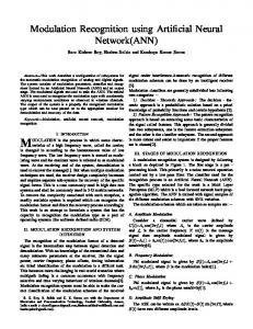
• Constellation: presents the values obtained by sampling the I and Q components at the time instants given by the receiver clock. A constellation diagram thus presents the actual received symbol values (Fig.1a); • Vector diagram: presents in the I − Q plane the whole trajectory of the vector associated with the demodulated signal. To obtain a vector diagram the I and Q components must be sampled at a higher rate than the receiver clock rate (Fig.1b). Q
Q
I
I
(a)
(b)
Fig. 1: I − Q diagrams: a) constellation; b) vector diagram.
From a measurement point of view, the main difference between the two diagrams lies in the different way of sampling the signal. To obtain a constellation diagram, the receiver clock must be available and determines the sampling instants. This may be provided by the system under test as an external clock input, or may be recovered by the measuring instrument from the analysed signal itself. In this way, by obtaining the number of clusters created in I − Q plane, levels and type of modulation could be identified. To the knowledge of author, one work on constellation diagram is reported by [6, 7], which is worked on fuzzy system. In [6, 7], fuzzy c-means clustering is used for initial processing but for final decision, it used a kind of template matching which uses a maximum likelihood approach. In this paper modulated signal symbols constellation utilizing TTSAS clustering algorithm and matching with standard templates is used for classification of QAM modulation. TTSAS algorithm used here is implemented by Hamming neural network. The simulation results show the capability of this method for modulation classification with high accuracy and appropriate convergence in the presence of noise.
3. TTSAS Clustering Algorithm Implemented by Hamming Neural Network In this paper, in order to cluster data symbols in I − Q plane, TTSAS (Two Threshold Sequential Algorithmic Scheme) clustering algorithm [19] has been used. The algorithm is implemented by Hamming neural network. Hamming neural network consists of two layers in which the first layer is score generator and the second is used to choose the best score [19, 20]. Weights of the first layer represent the centroids of created clusters. These weights are refreshed in each iteration of network training, until at the end of network training, the optimum weights (i.e. clusters) could be achieved. At the beginning of the TTSAS algorithm there is no need to prior knowledge of the number of clusters and it’s only needed to determine the maximum number of clusters and two thresholds. The algorithm begins with a single cluster and at the beginning this cluster is considered as a node in the hamming neural network and then the first data symbol is applied to the network, the weights at this node is in fact equal to the I − Q components of this data symbol. Therefore the first 45
N EGAR A HMADI
data symbol represents centroid of the first cluster. Then, data symbols are applied to the network sequentially. Each symbol which has been classified, its class tag is set to one. A symbol can be classified as one of the available classes or it introduces a new class or it’s postponed. If one of the first Two above conditions is satisfied the symbol is tagged one, otherwise it’s tag is set to zero and it could be classified in future iterations of the algorithm. The algorithm is repeated until all the symbols are classified, also if in one of iterations no symbol is classified, the algorithm is terminated. The Euclidean distances between each applied symbol with the centroids of available clusters are calculated and the shortest distance which corresponds to applied symbol, is chosen. First, this distance is compared with the first threshold and if its value is less than the threshold, this symbol is classified to the corresponding cluster and the centroid of the cluster is refreshed by averaging. If this condition doesn’t hold and the distance value is more than the first threshold, this distance is compared with the second threshold, if it’s value is greater than the second threshold and the number of clusters had not reached it’s maximum, this symbol introduces a new cluster, but if this value is between these two thresholds, it’s postponed to be assessed in future iterations of the algorithm. The next symbols are introduced similarly to the network. After the algorithm’s termination condition has been satisfied, a refinement step for optimizing the clusters obtained from TTSAS algorithm is performed, in order to accomplish this, first, clusters with a few members are eliminated and the near clusters are merged together. In the merging step, pair-wise distances of the centroids of the clusters are calculated and in each iteration two closest clusters are merged and the centroid of the new cluster is refreshed by averaging. This step is repeated until the number of obtained clusters equals to the number of constellation points of the modulation which is processed in the main program.
4. Neural Network Implementation In this section, neural network architecture is introduced and is then used to implement TTSAS. 4.1 Description of the Architecture The neural network architecture and implementation of the TTSAS algorithm used in this paper are illustrated in Fig.2a and Fig.2b.
S(x) Max Net (MN) Clastering Algorithm
Max Net (MN)
Matching Score Generator (MSG)
(b)
(a)
Fig. 2: a) The neural network architecture, b) Implementation of the TTSAS algorithm.
46
J OURNAL
OF
PATTERN R ECOGNITION R ESEARCH
The architecture consists of two modules, the matching score generator (MSG) and the Max Net network (MN). The first module stores q parameter vectors w1 , w2 , ..., wq of dimension l×1 and implements a function f (x, w), which indicate the similarity between x and w. The higher the value of f (x, w), the more similar x and w are. When a vector x is presented to the network, the MSG module outputs a q×1 vector ν, which its ith coordinate being equal to f (x, wi ), i = 1, ..., q. The second module takes as input the vector ν and identifies its maximum coordinate. Its output is a q×1 vector s with all its components equal to 0 except on the correspond to the maximum coordinate of ν. This is set equal to 1. Most of the modules of this type require at least one coordinate of ν to be positive. Different implementations of the MSG can be used, depending on the proximity measure adopted. For example, if the function f is the inner product, the MSG module consists of q linear nodes with their threshold being equal to 0. Each of these nodes is associated with a parameter vector wi , and its output is the inner product of the input vector x with wi . If the Euclidean distance is used, the MSG module consists also of q linear nodes. However, a different setup is required. The weight vector associated with the ith node is wi and its threshold is set equal to Ti = 0.5×(Q − kwi k2 ), where Q is a positive constant that ensures that at least one of the first layer nodes will output a positive matching score, and kwi k is the Euclidean norm of wi . Thus, the output of the nodes is: f (x, wi ) = xT wi + 0.5×(Q − kwi k2 )
(1)
The pseudo code of the TTSAS algorithm is shown in Fig.3. It is easy to show that d2 (x, wi ) < d2 (x, wj ) is equivalent to f (x, wi ) > f (x, wj ) and thus the output of MSG corresponds to the wi with the minimum Euclidean distance from x. The MN module can be implemented via a number of alternatives. One can use either neural network comparators such as the Hamming MaxNet and other feed-forward architectures or conventional comparators [19].
47
N EGAR A HMADI
The Two-Threshold Sequential Algorithmic Scheme (TTSAS) M=0 Class(x)=0 ∀x ∈ X Prev change=0 Cur change=0 Exists change=0 While (there exists at least one feature vector x with class(x)=0) do For i=1 to N If class(xi )= 0 AND it is the first in the new while loop AND exists change=0 then m = m+1 Cm ={xi } class(xi ) = 1 cur change = cur change + 1 Else if class(xi ) = 0 then Find d(xi , Ck ) = Min1≤j≤m d(xi , Cj ) If d(xi , Ck ) Θ1 then m = m+1 Cm ={xi } class(xi ) = 1 cur change = cur change + 1 End {if} Else if class(xi ) = 1 then cur change = cur change + 1 End {if} End {For} exists change = |cur change - prev change| prev change = cur change cur change = 0 End {While} Fig. 3: The TTSAS algorithm.
4.2 Description of the Architecture In this section, we demonstrate how the TTSAS algorithm can be mapped to the neural network architecture when (a) each cluster is represented by its mean vector and (b) the Euclidean distance between two vectors is used (Fig 2-b). The structure of the Hamming network must also be slightly modified, so that each node in the first layer to have as an extra input the term −0.5kxk2 . Let wi and Ti be the weight vector and threshold of the ith node in the MSG module, respectively. Also let a be a q×1 vector whose ith component indicates the number of vectors contained in the ith cluster. Also, let s(x) be the output of the MN module when the input to the network is x. In addition, let ti be the connection between the ith node of the MSG and its corresponding node in the MN module. Finally, let sgn(z) be the step function that returns 1 if z > 0 and 0 otherwise. 48
J OURNAL
OF
PATTERN R ECOGNITION R ESEARCH
The first m of the q wi ’s correspond to the representatives of the clusters defined so far by the algorithm. At each iteration step either one of the first m wi ’s is updated or a new parameter vector wm+1 is employed, whenever a new cluster is created (if m < q). The algorithm may be stated as follows. • Initialization *a = 0, m = 1, wi = 0, ti = 0 ∴ i = 1, ..., q - For the first vector xi set * wi = x1 , a1 = 1, t1 = 1 • Main Phase - Repeat * Present the next vector to the network * Compute the output vector s(x) q P * GAT E(x) = AN D((1 − (sj (x))), sgn(q − m)) j=1
* m = m + GAT E(x), am = am + GAT E(x) * wm = wm + GAT E(x), Tm = Θ − 0.5×kwm k2 , tm = 1 * For j = 1 to m • aj = aj + (1 − GAT E(x))sj (x) • wj = wj + (1 − GAT E(x))sj (x)((wj − x)/aj ) • Tj = Θ − 0.5×kwm k2 • Next j - Until all vectors have been presented once to have network. Note that only the outputs of the m first nodes of the MSG module are taken into account, because only these correspond to clusters. The outputs of the remaining nodes are not taken to accounts, since tk = 0, k = m + 1, ..., q. Assume that a new vector is presented to the network such that min1≤j≤m d(x, wi ) > Θ and m < q then GAT E(x) = 1. Therefore, a new cluster is created and the next node is activated in order to represent it. Since (1 − GAT E(x)) = 0, the execution of the instruction in the F or loop does not affect any of the parameters of the network. Suppose next that GAT E(x) = 0. This equivalent to the fact that either min1≤j≤m d(x, wi ) ≤ Θ or there are no more nodes available to represent additional clusters. Then the execution of the instructions in the F or loop results in updating the weight vector and the threshold of the node, k for which min1≤j≤m d(x, wi ). This happens because sk (x) = 1 and sj (x) = 0, j = 1, ...q, j 6= k .
5. Recognition of QAM Modulation using TTSAS Algorithm and Template Matching Fig.4 shows the flowchart of the proposed method for recognition of modulation. At first, the ideal constellation points for each modulation type of QAM family are determined. It should be noted that only the points which lie in the first quadrant of the constellation have been considered, one point is determined for 4-QAM and 4, 16 and 64 points for 16 - 64 and 256-QAM, respectively. The determined points are normalized in the interval of [0, 1]. In order to compare the centroids of the clusters resulted from the symbols with ideal points of the constellation, the absolute values of I −Q components of each symbols are calculated and then these values are normalized. Evaluation begins with 256-QAM and finishes with 4-QAM. After the clusters are determined by TTSAS algorithm, the template matching is performed. 49
N EGAR A HMADI
START Define Ideal Centroids for each type of modulation (4, 16, 64, 256-QAM)
Set modulation type for evaluation
Set initial parameters of TTSAS algorithm based on modulation type: Two thresholds = T1, T2 and N= final number of clusters
Run TTSAS algorithm and obtain centroids
Compute similarity value between ideal centroids and centroids derived from TTSAS algorithm
NO
Judgment and Termination: If (similarity < threshold)
YES Recognized modulation type = current modulation type
END Fig. 4: The flowchart of propose method.
In the template matching stage, the resulted clusters are matched with the ideal points of QAM modulations. In the first iteration of the main algorithm, matching with 256-QAM is evaluated. This comparison is made by calculation of Euclidean distance between the corresponding centroids of the clusters and the ideal points of the modulation type. then this distance is compared with a threshold which is determined for 256-QAM, if the distance is less than the threshold, 256-QAM is presented as recognized modulation and the main program is terminated, else, if this condition doesn’t hold, the next type (i.e. 64-QAM) is considered for the evaluation and the algorithm is executed again. If the matching condition is satisfied, 64-QAM is presented as recognized modulation and the main algorithm is terminated, else the evaluation is done for 16-QAM in similar manner. If none of the three evaluated types are presented as recognized modulation, the 4-QAM is assumed and presented as recognized modulation. The pseudo code of creating templates is shown in Fig.5.
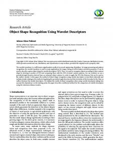
6. Performance Evaluation and Simulation Results To evaluate the proposed method, simulation for different values of noise and different modulation of QAM and PSK families have been conducted. Channel model, applied in this work, has been assumed to be an AWGN channel, and it is also assumed that there is no time and/or frequency synchronization error. Simulation results show a high efficiency and accuracy in recognition of different types of modulations. Figures Fig.6a to Fig.6c show centroids resulted from TTSAS algorithm in first quadrant for 16QAM, 64 QAM and 256 QAM with various SNR and comparison with the relevant templates. As it’s seen, the accuracy of this method is extremely high so it is a suitable method for recognition of 50
J OURNAL
OF
PATTERN R ECOGNITION R ESEARCH
% Ideal Centroids : cent1=[.5, .5]; % 4-QAM cent4=[1, 1; 1, 3; 3, 1; 3, 3]/4; % 16-QAM %- - - - - - 64-QAM k=0; for i=1:2:7 for j=1:2:7 k=k+1; cent16(k,:)=[i, j]; end end cent16=cent16./8; %——– 256-QAM k=0; for i=1:2:15 for j=1:2:15 k=k+1; cent64(k,:)=[i,j]; end end cent64=cent64./16; Fig. 5: Pseudo code of creating templates
QAM family modulation. Figures Fig.7a to Fig.7d demonstrate data symbols and resulted centroids after recognition of modulation. Because there was some possibility in appearance of errors in post processing stage in other methods, by using the template matching method we try to reduce the error and increase the accuracy of modulation recognition in the presence of noise. In this method by defining standard model of constellations of every modulation and comparing them to resultant constellation from fuzzy method or genetic algorithm and by using template matching, we succeed in differentiation between modulations with a high accuracy. In this method, in a case of using fuzzy method or genetic algorithm method we should identify the number of clusters and initial value of their centriods for different modulations and because the initial values have an important role in the rate of algorithm convergence, by using TTSAS algorithm we solve this problem. For operating this algorithm a neural Hamming network was used which is dual layer network that the first layer is for the calculation of mark and the second layer is used for choosing the best mark. The results from this method have verified its high accuracy in recognition of modulations and good rate of convergence. The accuracy of the recognition of modulation in low signal to noise values in this method because of the using of template was increased in a great amount. By using of TTSAS algorithm, there is no need to know the number of clusters and their initial value; it was a great advantage in using TTSAS algorithm. In this method in low signal to noise values, with increasing the number of input samples the accuracy of modulation recognition was increased. For recognition of these types of modulation with various SNR, different number of samples are used which are presented in Table 1, Table 2 and Fig.8 present the accuracy percentage of the modulation recognition versus SNR, for various types. The accuracy percentages have been obtained by executing algorithm enough times and calculating the ratio between correct recognition and total number of execution. 51
N EGAR A HMADI
1.0
1.0
0.8
0.8
0.6
0.6
0.4
0.4
0.2
0.2
0
0.2
0.4
0.8
0.6
0
1.0
0.2
0.4
(a)
0.6
0.8
1.0
(b) Detected Centroids
1.0
Ideal Centroids 0.8
0.6
0.4
0.2
0
0.2
0.4
0.6
0.8
1.0
( c)
Fig. 6: Centroids resulted from TTSAS algorithm in first quadrant and comparison with the ideal centriods for a) 16QAM with SNR=3dB, b) 64-QAM with SNR=9dB, c) 256-QAM with SNR=20dB.
Jiang Yuan and et al [21] presented a classifier using wavelet transform and pattern recognition technique to discriminate some analogue and digital modulations. Their proposed classifier has classification accuracy for 16-QAM at the SNR>15. For example their method recognized 16QAM with 0.90 accuracy in SNR=10db and 0.91 in SNR=15. In another research Hong Li and et al [22] employed a quasi - hybrid likelihood ratio test approach to classify signal with unknown carrier frequency offset. A blind symbol-rate-sampling nonlinear least-squares CFO estimator is incorporated in the qHLRT algorithm. They observed that when SNR increases, the transmitted 64-QAM can be accurately recognized, whereas 4-QAM and 16QAM are falsely treated as 64-QAM. In addition to above articles, some researches with various methods of classification were presented in [23, 24]. In compression with all of the previous presented results, my proposed method shows a good recognition performance even in extremely low SNR condition for 4-QAM, 16-QAM, 64-QAM and 256-QAM. Another advantage of this method is calculating final centroids of the clusters and determining the location of these centroids in constellation diagram. In addition this approach could be extended and modified to recognize other types of digital modulation.
52
J OURNAL
OF
PATTERN R ECOGNITION R ESEARCH
200
400
100
200
0
0
-100
-200
-200 -200
-100
100
0
-400 -400
200
-200
(a)
0
200
400
1000
2000
(b) 2000
800 1000
400
0
0
-400 -1000
-800 -800
-400
0
400
-2000 -2000
800
-1000
(c)
0
(d)
Fig. 7: Data symbols and resulted centroids after recognition of a) 4-QAM with SNR=2dB, b) 16-QAM with SNR 3dB, c) 64-QAM with SNR=9dB and d) 256-QAM with SNR=20dB. Table 1: Number of samples for modulation recognition with various SNR
256-QAM
SNR Number of Samples
30dB 1000
25dB 1000
20dB 1500
19dB 2000
18dB 8000
17 dB 22000
64-QAM
SNR Number of Samples
25dB 1000
20dB 1000
17dB 1000
15dB 1000
12dB 7000
10 dB 7000
16-QAM
SNR Number of Samples
15dB 1000
12dB 1000
10dB 1000
8dB 1000
5dB 1000
3dB 5000
4-QAM
SNR Number of Samples
10dB 1000
5dB 1000
3dB 1000
1dB 1000
0dB 1000
-2dB 1000
Table 2: Extended Accuracy percentage of recognition versus SNR
SNR (dB)
0
3
5
10
15
17
20
4-QAM 16-QAM 64-QAM 256-QAM
100 35 5 2
100 100 15 3
100 100 40 8
100 100 100 20
100 100 100 75
100 100 100 100
100 100 100 100
53
N EGAR A HMADI
100
Accuracy Percentage
80
60
40 4 - QAM 16 - QAM 64 - QAM 256 - QAM
20
0
0
5
10
15
20
25
30
SNR in dB Fig. 8: Accuracy percentage of recognition versus SNR
7. Conclusion In this paper, by utilizing TTSAS clustering algorithm, which is implemented by Hamming neural network, we obtained the centroids of clusters which are created automatically in I − Q plane, then by evaluating the amount of matching with the standard templates of QAM modulations, we can recognize the type of modulation. Because of using both clustering algorithm and template matching, the sensitivity of this method with respect to the noise has been reduced. As can be seen in simulation section, the proposed method shows a good recognition performance even in low SNR condition, of course, it must be mentioned that the performance could be improved with higher number of data symbols. Another advantage of this method is calculating final centroids of the clusters and determining the location of these centroids in constellation diagram. In addition this approach could be extended and modified to recognize other types of digital modulation. The method that have been used can be expanded and use them for modulation recognition of any PAM signals. These signals have one dimensional constellation while in this research we study the signals with two dimensional constellations which are more complicated. Thus with a little change we can use them for recognition of PAM signals. From these signals the MFSK and MASK modulations can be referred. With little changes in proposed method it can be used in recognition of modulations which have non standard one dimensional or two dimensional constellations. By rotating the constellation diagram of PAM signals for 45◦ in I − Q plane, without any change in proposed method, it can recognize modulations.
54
J OURNAL
OF
PATTERN R ECOGNITION R ESEARCH
References [1] J. Lopatka and M. Pedzisz, ”Automatic Modulation Classification using Statistical Moments and a Fuzzy Classifier”, Signal Processing Proceedings, WCCC- ICSP 2000, 5th international conf. on, 2125 Aug. 2000, Vol.3, pp. 1500-1506. [2] Y. O. Al-Jalili , ”Identification Algorithm of Upper Sideband and Lower Sideband SSB Signals” , Signal Processing , Vol. 42, 1995, pp. 207-213. [3] L. Narduzzi, M. Bertocco, ”Conformance and Performance”, Department of Electronic and Informatics, Pavova University, 2003. [4] J. Reichert, ”Automatic Classification of Communication Signals using Higher Order Statistics”, ICASSP 92, pp.221-224. [5] R. Schalkoff, ”Pattern Recognition: Statistical, Structural and Neural Approach” 1992, John Wiley. [6] Bijan G. Mobaseri, ”Constellation shape as a robust signature for digital modulation recognition”, Military Communications Conference Proceedings, MILCOM IEEE, Volume 1, Issue, 1999, pp. 442-446. [7] Bijan G. Mobasseri, ”Digital Modulation Classification using Constellation Shape”, Signal Processing, Vol. 80, No. 2, 2000, pp.251-277. [8] F. Jondral, ”Automatic Classification of High Frequency Signals”, Signal Processing, Vol. 9, No. 3, 1985, pp.177-190. [9] L. Dominguez, J. Borrallo, J. Garcia, ”A General Approach to the Automatic Classification of Radiocommunication Signals”, Signal Processing, Vol. 22, No. 3, 1991, pp.239-250. [10] F.F. Liedtke, ”Computer Simulation of an Automatic Classification Procedure for Digitally Modulated Communication Signals with Unknown Parameters”, Signal Processing, Vol. 6, 1984, pp.311.323 [11] J. Aisbett, ”Automatic Modulation Recognition using Time-Domain Parameters”, Signal Processing, Vol.13, No. 3, 1987, pp.323-329. [12] A. Polydoros, K. Kim, ”On the Detection and Classification of Quadrature Digital Modulation in BroadBand Noise”, IEEE Transactions on Communications, Vol. 38, No. 8, August 1990, pp. 1199-1211. [13] C. Huang, A. Polydoros, ”Likehood Method for MPSK Modulation Classification”, IEEE Transaction on Communications, Vol. 43, No. 2/3/4, 1995, pp.1493-1503. [14] S. Soliman, S. Hsue, ”Signal classification using statistical moments”, IEEE Transactions on Communications, Vol. 40, No. 5, May 1992, pp. 908-915. [15] W. Wei, J. Mendel, ”A New Maximum Likelihood for Modulation Classification,” Asilomar-29, 1996, pp. 1132-1138. [16] K. Chugg, et al, ”Combined Likelihood Power Estimation and Multiple Hypothesis Modulation Classification”, Asilomar-29, 1996, pp. 1137-1141. [17] Y.Lin, C.C. Kuo, ”Classification of Quadrature Amplitude Modulated (QAM) Signals via Sequential Probability Ratio Test (SPRT)”, Report of CRASP, University of Southern California, July 15, 1996. [18] Nhi P. Ta, ”A Wavelet Packet Approach to Radio Signal Classification”, symposium on Time-Frequency and Time Scale Analysis, 1994, pp. 508-511. [19] S. Theodoridis, K. Koutroumbas, ”Pattern Recognition”, Elsevier Academic Press, Second Edition, 2003. [20] E. Gose, R. Johnsonbaugh, S. Jost, ”Pattern Recognition and Image Analysis”, Prentice Hall PTR, 1996. [21] J. Yuan, Z. Zhao-Yang, Q. Pei-Liang, ”Modulation Classification of Communication’ Signals”, MILCOM 2004 -IEEE Military Communications Conference, 31 Oct-3 Nov 2004, pp 1470-1476. [22] H. Li, O. A. Dobret, Y. Bar-Ness, W. Su, ”Quasi-Hybrid Likelihood Modulation Classification with Nonlinear Carrier Frequency Offsets Estimation using Antenna Arrays”, MILCOM 2005 -IEEE Military Communications Conference, 17-20 Oct. 2005, Vol. 1, pp 570-575. [23] O. A. Dobre, A. Abdi, Y. Bar-Ness, W. Su, ”The Classification of Joint Analog and Digital Modulations”, MILCOM 2005 -IEEE Military Communications Conference, 17-20 Oct. 2005, Vol. 5, pp 3010-3015. [24] Wu Dan, Gu Xuemai, Guo Qing, ”Classification using a Novel Support Vector Machine Fuzzy Network for Digital Modulations in Satellite Communication”, Wireless Communications, Networking and Mobile Computing, 2005. Proceedings, International Conference on, Volume 1, 23-26 Sept. 2005, pp. 508-512.
55