New Methodologies Based on Delta Test for Variable Selection in Regression Problems Alberto Guill´en, Dusan Sovilj, Fernando Mateo, Ignacio Rojas and Amaury Lendasse
Abstract— The problem of selecting an adequate set of variables from a given data set of a sampled function, becomes crucial by the time of designing the model that will approximate it. Several approaches have been presented in the literature although recent studies showed how the Delta Test is a powerful tool to determine if a subset of variables is correct. This paper presents new methodologies based on the Delta Test such as Tabu Search, Genetic Algorithms and the hybridization of them, to determine a subset of variables which is representative of a function. The paper considers as well the scaling problem where a relevance value is assigned to each variable. The new algorithms were adapted to be run in parallel architectures so better performances could be obtained in a small amount of time, presenting great robustness and scalability.
I. I NTRODUCTION
I
N many real-life problems it is convenient to reduce the number of involved features (variables) in order to reduce the complexity, especially when the number of features is large compared to the number of observations (e.g. finance problems, weather forecast, electricity load prediction, etc.). There are several criteria to tackle this variable reduction problem. Three of the most common are: maximization of the mutual information (MI) between the inputs and the outputs, minimization of the k-nearest neighbors (k-NN) leave-one-out generalization error estimate and minimization of a nonparametric noise estimator (NNE). The problem of regression or function approximation consists in, given a set of input vectors with their corresponding output, it is desired to build a model that learns the relationship between the input variables and the output variable. Formally this problem can be enunciated as, given a set of observations {(~xj ; yj ); j = 1, ..., N } with yj = F (~xj ) ∈ R and ~xj ∈ Rd , it is desired to obtain a function G so yj = G (~xj ) ∈ R with ~xj ∈ Rd . There exists a wide variety of models that are able to approximate any function such as Neural Networks [1], [2], Fuzzy Systems [3], Support Vector Machines (SVM) and Least Square SVM [4], etc. however, they all suffer from the Curse of Dimensionality [5]. As the number of dimensions d grows, the number of input values required to sample the solution space increases exponentially, this means that the Alberto Guill´en and Ignacio Rojas are with the Department of Computer Architecture and Technology, University of Granada, Spain (email:
[email protected]). Fernando Mateo is with the Department of Electronic Engineering, Polytechnic University of Valencia, Spain. Dusan Sovilj and Amaury Lendasse are with the Department of Information and Computer Science, Helsinki University of Technology, Finland. This work has been partially supported by the projects TIN2007-60587, P07-TIC-02768 and P07-TIC-02906, and by research grant BES-2005-9703 from the Spanish Ministry of Science and Innovation.
models will not be able to set their parameters correctly if there are not enough input vectors in the training set. Many real- life problems present this drawback since they have a considerable amount of variables to be selected in comparison to the few number of observations. Thus, efficient and effective algorithms to reduce the dimensionality of the data sets are required. The literature presents a wide number of methodologies for feature or variable selection ([6], [7], [8]) although they have been focused on classification problems. Regression problems differ from classification since: • The output of the problem is continuous, not like in classification, where a finite number of classes is defined a priori. • There is a proximity between different outputs, not like in classification, where classes (in general) cannot be related. Therefore, specific algorithms for this kind of problem must be designed. Recently, it has been demonstrated in [9] how the Delta Test (DT) is a quite powerful tool to determine the quality of a subset of variables using ForwardBackward optimization. However, there are other alternatives that allow to perform a global optimization of the variable selection like Genetic Algorithms (GA) [10] and Tabu Search (TS) [11]. One of the main drawbacks of using global optimization techniques is their computational cost. Nevertheless, the latest advances in computer architecture provide powerful clusters without requiring a large budget, so an adequate parallelization of these techniques might ameliorate this problem. This is quite important in real-life applications where the response time of the algorithm must be acceptable from the perspective of a human operator. This paper presents several new approaches to perform variable selection using the DT as criterion to decide if a subset of variables is adequate or not. The new approaches are based in local search methodologies, global optimization techniques and the hybridization of both. The rest of the paper is structured as follows: Section 2 introduces the DT and its theoretical framework, then, Section 3 describes the previous methodology to perform the variable selection as well as the new developed algorithms. Section 4 presents a complete experimental study analyzing the behavior of the algorithms and, in Section 5, conclusions are drawn. II. E QUIVALENT R EFORMULATIONS The Delta Test (DT), firstly introduced by Pi and Peterson for time series [12] and proposed for variable selection in [9], is a technique to estimate the variance of the noise, or
the mean squared error (MSE), that can be achieved without overfitting. Given N input-output pairs (xi , yi ) ∈ Rd × R, the relationship between xi and yi can be expressed as: yi = f (xi )+ri , i = 1, ..., N , where f is the unknown function and r is the noise. The DT estimates the variance of the noise r. The DT is useful for evaluating the nonlinear correlation between two random variables, namely, input and output pairs. The DT can be also applied to input variable selection: the set of input variables that minimizes the DT is the one that is selected. Indeed, according to the DT, the selected set of input variables is the one that represents the relationship between input variables and the output variable in the most deterministic way. DT is based on hypothesis coming from the continuity of the regression function. If two points x and x′ are close in the input variable space, the continuity of regression function implies the outputs f (x) and f (x′ ) will be close enough in the output space. Alternatively, if the corresponding output values are not close in the output space, this is due to the influence of the noise. The DT can be interpreted as a particularization of the Gamma Test [13] considering only the first nearest neighbor. Let us denote the first nearest neighbor of a point xi in the Rd space as xN N (i) . The nearest neighbor formulation of the DT estimates Var[r] by Var[r] ≈ δ =
N 1 X (yi − yN N (i) )2 , 2N i=1
with Var[δ] → 0 for N → ∞ where yN N (i) is the output of xN N (i) . III. VARIABLE S ELECTION M ETHODOLOGIES This Section presents the previous methodology proposed to compute the minimum value for the DT, the ForwardBackward Search. Then, it presents an adaptation of the TS for the minimization of the DT. Finally, a new algorithm that combines the TS and the global optimization capabilities of GA is introduced. The methodologies described below are applied to the problem of variable selection from two perspectives: binary and scaled. The binary approach considers a solution as a set of binary values that indicate if that variable is relevant or not. The scaled approach assigns a weighting factor to each variable according to its importance. The scaling problem is more challenging because the solution space grows considerably. A. Forward-Backward Search To overcome the difficulties and the high computational time that an exhaustive search would entail (i.e. 2d − 1 input variable combinations, being d the number of variables), there are several other search strategies. These strategies are affected by local optima because they do not test every input variable combination. Among the typical search strategies, there are three that share similarities: Forward Search, Backward Search (or pruning), and Forward-Backward Search.
The difference between the first two is that the Forward Search starts from an empty set of selected variables and adds variables to it according to the optimization of a search criterion, while the Backward Search starts from a set containing all the variables and removes those for which the elimination optimizes the search criterion. Both Forward and Backward Search suffer from incomplete search. The Forward-Backward Search (FBS) is a combination of them. It is more flexible in the sense that a variable is able to return to the selected set once it has been dropped, and vice versa, a previously selected variable can be discarded later. This method can start from any initial input variable set: empty set, full set, custom set or randomly initialized set. If we consider a set of N input-output pairs (xi , yi ) ∈ Rd × R, the FBS algorithm can be described as follows 1) Initialization: Let S be the selected input variable set, which can contain any input variables, and F the unselected input variable set, which contains the variables not present in S. Compute Var[r] using Delta Test on the set S. 2) Forward-Backward selection step: Find the variable xS to include or to remove from the set S to minimize Var[r]: xS = arg minxi ,xj {(Var[r]|S ∪ xj ) ∪ (Var[r]|S \ xi )}, xi ∈ S, xj ∈ F 3) If the old value of Var[r] on the set S is lower than the new result, stop; otherwise, update set S and save the new Var[r]. Repeat step 2 until S is equal to any former selected S. 4) The selected input variable set is S B. Tabu Search Tabu Search (TS) is a metaheuristic method designed to guide local search methods to explore the solution space beyond local optimality. The first most successful usage was by Glover in [14] for combinatorial optimization. Later TS was successfully used in scheduling [15], [16], routing [17] and general optimization problems [18]. In general, the problem is in form of an objective or cost function f (v), given the set of solutions v ∈ V . In the context of TS, the neighborhood relationship between solutions, denoted N e(v), plays the central role. While there are other neighborhood based methods, such as descent/ascent methods widely used, the difference is that tabu uses memory in order to influence which parts of the neighborhood are going to be explored. A memory is used to record various aspects of the search process and the solutions encountered, such as recency, frequency, quality and influence of moves. The most important aspect of the memory is to forbid some moves to be applied, or in other words, to prevent the search to go back to solutions that were already visited. This also allows the search to focus on such moves that guide the search toward unexplored areas of the solutions space. This part of the memory is called a tabu list, and the moves in
this list are then considered tabu, and thus forbidden to use. The size of the tabu list as well as the time each move is kept in the list are important issues in TS. These parameters should be set up so that the search is able to go through two distinct, but equally important phases: intensification and diversification. As far as we know, no implementation of the TS to minimize the DT has ever been done, so it was implemented in this work as an improvement over the FBS, which does not have any memory enhancement. Due to the fact that this paper considers the variable selection and the scaling problem, two different algorithms had to be designed. Both algorithms use only short-term recency based memory to store reverse moves instead of solutions to speedup the exploration of the search space. 1) TS for pure variable selection: In the case of variable selection, a move was defined as a flip of the status of exactly one variable in the data set. The status is excluded (0) or included (1) from the selection. For a data set of dimensionality d, a solution is then a vector of zeros and ones v = (v1 , v2 , . . . , vd ), where vk ∈ {0, 1} , k = 1, ..., d, are indicator variables representing the selection status of kth dimension. The neighborhood of a selection (solution) v is a set of selections u which have exactly one variable that has different status. This can be written as N e(v) = {u | ∃1 q ∈ {1, . . . , d} vq 6= uq ∧ vi = ui , i 6= q} With this setup, each solution has exactly the same amount of neighbors, which will be equal to d. 2) TS for the scaling problem: The first modification that requires the adaptation to the scaling problem is the definition of the neighborhood of a solution. A solution v is now a vector with scaling values from a discretized set vk ∈ H = {0, 1/k, 2/k, . . . , 1}, where k is discretization parameter. Two solutions are neighbors if they disagree on exactly one variable, same as for variable selection, but the disagreement is the smallest possible value. N e(v) is defined in a same way as for variable selection, but with an additional constraint of |vq − uq | = 1/k. For example, for k = 10 and d = 3, the solutions v1 = (0.4, 0.2, 0.8) and v2 = (0.3, 0.2, 0.8) would be neighbors, but not the solution v3 = (0.1, 0.2, 0.8). The move between solutions is defined as a change of value for one dimension, which can be written as a vector (dimension, old value, new value). 3) Setting the tabu conditions: The tenure for a move is defined as the number of iterations that it is considered as tabu. This value is determined empirically when the TS is applied to solve a concrete problem. For the variable selection problem, this paper proposes a value which is dependent on the number of dimensions so it can be applied to several problems. In the experiments, two tabu lists, and thus two tenures, were used. The first list is responsible for preventing the change along certain dimension for d/4 iterations. The second one prevents the change along the same dimension and for specified scaling value for d/4 + 2
iterations. The combination of these two lists gave better results than when each of the conditions was used alone. For example, for k = 10, if a move is performed along dimension 3 from value 0.1 to 0.2, which can be written as a vector m = (3; 0.1, 0.2), then its reverse move m−1 = (3; 0.2, 0.1) is stored in the list. The search will be forbidden to use any move along dimension 3 for d/4 + 2 iterations, and after that time, it will be further 2 iterations restricted to use the move m−1 , or in other words to go back from 0.2 to 0.1. With these settings, in the case of variable selection, two conditions are then implicitly merged into one condition: restrict a flip of the variable for d/4 + 2 iterations. This is because there are only two values 0,1 as possible choices. C. Hybrid Parallel Genetic Algorithm The benefits and advantages of the global optimization and local search techniques have been hybridized in the proposed algorithm. The idea is to be able to have a global optimization, using a GA, but still being able to make a fine tune of the solution, using the TS. The following paragraphs describe the different elements that define the algorithm. 1) Encoding of the individuals and initial population: Deciding how a chromosome encodes a solution is one of the most decisive design steps since it will influence the rest of the design [19]. The classical encoding used for variable selection has been a vector of binary values where 1 represents that the variable is selected and 0 that the variable is not selected. Since this paper considers the variable selection using scaling, instead of using binary values, other encoding must be chosen. If the algorithm uses real numbers to determine the weight of a variable, it could fall into the category of Real Coded Genetic Algorithms (RCGA). However, the number of scales has been discretized in order to bound the number of possible solutions making the algorithm a classical GA where the cardinality of the alphabet for the solutions is increased in k values. For the sake of simplicity in the implementation, an individual is a vector of integers where the number 1 represents that the variable was selected and k + 1 means that the variable is not selected. Regarding the initial population, some individuals are included in the population deterministically to ensure that each scaling value for each variable exists in the population. These individuals are required if the classical GA crossover operators (one/two-points, uniform) are applied so all the possible combinations can be reached. For example, if the number of scales is 4 in a problem with 3 variables, the individuals that are always included in the population are: 1 1 1, 2 2 2, 3 3 3, and 4 4 4. 2) Selection, crossover and mutation operators: The algorithm was designed in order to be as fast as possible so when several design options appeared, the fastest one (in terms of computation time) was selected, as long as it was reasonable. The selection operator chosen was the binary tournament selection as presented by Goldberg in [20] instead of the Baker’s roulette wheel operator [21] or other
more complex operators existing in the literature. The reason for this is because the binary tournament does not require the computation of any probability for each individual, thus, a considerable amount of operations are saved on each iteration. This is specially important for large populations. Furthermore, the fact that the binary tournament does not introduce a high selective pressure is not as traumatic as it might seem. The reason is because the huge solution space, that arises as soon as the number of scales increases, should be deeply explored to avoid local minima. Nevertheless, the algorithm incorporates the elitism mechanism, keeping the 10% of the best individuals of the population, so the convergence is still feasible. Regarding the crossover operator, the algorithm implemented the classical operators for a binary coded GA, these are: one-point and two-point crossovers and the uniform crossover [22], [10], [23]. The behavior of the algorithm using these crossovers was quite similar and acceptable. Nonetheless, since the algorithm could be included into the Real Coded GA class, an adaptation of the BLX-α [24] was implemented as well. The adaptation only required to round the absolute value assigned to each gene and also the modification of the value in case it is out of the bounds of the solution space. The mutation operates at a gene level, so a gene has the chance to get any value of the alphabet. 3) Parallelization: The algorithm has been parallelized so it is able to take advantage of the parallel architectures, like clusters of computers, that are easy available anywhere. The main reason to parallelize the algorithm is to be able to explore more solutions in the same time, allowing the population to reach a better solution. The fitness function still remains expensive in comparison with the other stages of the algorithm (selection, crossover, mutation, etc.). At first, all the stages of the GA were parallelized, but the results showed that the communication and synchronization operations could be more expensive than performing the stages synchronously and separately on each processor 1 . Hence, only the computation of the DT for each individual is distributed between the different processors in a master/slave topology quite similar to the ones proposed in the literature [25], [26]. The algorithm assumes that all processors are equal with the same amount of memory and speed. If they were not, it should be considered to send the individuals iteratively to each processors as soon as they were finished with the computation of the fitness of an individual. This is equivalent to the case where the fitness function computational time might change from one individual to another. However, the computation of the DT does not significantly vary from one individual to another, despite the number of variables they have selected. Thus, using homogeneous processors and constant time consuming fitness function, the amount of individuals that each processor should evaluate is 1 This paper considers that a processor will execute one process of the algorithm.
size of population/number of processors. The algorithm has been implemented so the number of communications (and their number of packets) is minimized. To achieve this, all the processors execute exactly the same code so, when each one of them has to evaluate its part of the population, it does not require to get the data from the master because it already has the current population. The only communications that have to be done during the execution of the GA are, after the evaluation of the individuals, to send and receive the values of the DT, but not the individuals themselves. To make possible that all processors have the same population all the time considering that there are random elements, at the beginning of the algorithm the master processor sends to all the others the seed for their random number generators. This implies that they all produce the same values when calling the function to obtain a random number. In this way, when the processors have to communicate, only the value of the DT computed will be sent, saving the communications that would require to send each individual to be evaluated. This is specially important since some problems require large individuals, increasing the traffic in the network and retarding the execution of the algorithm. 4) Hybridization: The combination of local optimization techniques with GA has been studied in several papers [27], [28], [29]. Furthermore, the inclusion of a FBS in a stage of an algorithm for variable selection was recently proposed in [7] but, the algorithm was oriented to classification problems. The new approach that this paper proposes is to perform a local search at the beginning and at the end of the GA. The local search will be done by using the TS described in the Section III-B, so it does not stop when it finds a local minimum. Using a good initialization as a start point for the GA, it is possible to find good solutions with smaller populations [30]. This is quite important because the smaller the population is, the faster the algorithm will complete a generation. Therefore, the algorithm incorporates an individual generated using the TS, so there is a potential solution which has a good fitness. Since the algorithm is able to use several processors, several TSs can be run on each processor. The processors will communicate sending each other the final individual once the TS is over. Afterwards, they will start the GA using the same random seed. Thus, if there are p processors, p individuals of the population will be generated using the TS. Thanks to the use of the binary tournament selection, there is no need to worry about converging too fast to a local minimum near these individuals. The GA will then explore the solution space and when it finishes, each processor will take an individual using it as the starting point for a new TS. In this way, the exploitation of a good solution is guaranteed. The first processor takes the best individual, the second, takes the second best individual and so on. As the GA maintains diversity in the population, the best result after applying the TS does not always come from the best individual in the population. This fact shows how important is to keep exploring the solution space instead of letting the
Cpu cores: 2, Bogomips: 3723.87, Clflush size: 64, Cache alignment: 64, Address sizes: 40 bits physical, 48 bits virtual. The algorithms were implemented in MATLAB and, in order to communicate the different processes, the MPImex ToolBox presented in [31] was used. A. Data sets used in the experiments
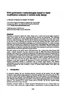
Fig. 1. Algorithm scheme. Dashed line represents one to one communication, dotted lines represent collective communications.
GA converge too fast. Figure 1 shows how the algorithm is structured as well as the communications that are necessary to obtain the final solution. IV. E XPERIMENTS AND
RESULTS
This Section will show empirically the performance of the algorithm. First, the data sets that have been used are introduced. Then, the effect of the parallelism applied over the GA will be analyzed. Afterwards, more experiments with the parallel version will be done in order to show how the addition of the BLX-α crossover and the TS can improve the results. Finally, the new proposed algorithm will be compared against the local search technique used so far, demonstrating how the global optimization, in combination with the local search, leads to better solutions. Nothing was commented so far about the stopping criterion of the algorithm. In the experiments, a time limit of 600 seconds for all the algorithms was used. The decision to set this time limit is because the experience when working with industries says that 10 minutes is the maximum amount of time that an operator is willing to wait. Furthermore, this value has been widely used in the literature as time limit. Two different clusters were used in the experiments but, due to the lack of space, only the results of the better one will be showed. Nonetheless, the algorithms had a similar performance in both of them. A remarkable fact was that the size of the cache was crucial by the time of computing the DT. Due to the large size of the distances matrix, the faster computer had a worse performance because it did not have as much cache memory as the other. The processors in the cluster used had the following characteristics: Cpu family: 6, Model: 15, Model name: Intel(R) Xeon(R) CPU E5320 @ 1.86GHz, Stepping: 7, Cpu MHz: 1595.931, Cache size: 4096 KB,
To assess the presented methods, several experiments were performed, using the following data sets: 1) The Housing data set2 is related to the estimation of housing values in suburbs of Boston. The value to predict is the median value of owner-occupied homes in $1000’s. The data set contains 506 instances, with 13 input variables and one output. 2)The Tecator data set3 aims at performing the task of predicting the fat content of a meat sample on the basis of its near infrared absorbance spectrum. The data set contains 215 useful instances for interpolation problems, with 100 input channels, 22 principal components (which will remain unused) and 3 outputs, although only one is going to be used (fat content). 3)The Anthrokids data set4 represents the results of a threeyear study on 3900 infants and children representative of the U.S. population of year 1977. The data set comprises 121 variables and the target variable to predict is children’s weight. As this data set presented many missing values, a prior sample and variable discrimination had to be performed to build a robust and reliable data set. The final set5 without missing values contains 1019 instances, 53 input variables and one output (weight). More information on this data set reduction methodology can be found in [32]. 4) The Santa Fe time series competition data set6 is a time series recorded from laboratory measurements of a Far-Infrared-Laser in a chaotic state. The set contains 1000 samples, and it was reshaped for its application to time series prediction using regressors of 12 samples. Thus, the set used in this work contains 987 instances, 12 inputs and one output. 5) The ESTSP 2007 competition data set5 : This time series was proposed for the European Symposium on Time Series Prediction 2007. It is an univariate set containing 875 samples but has been reshaped using a regressor of 55 variables, producing a final set of 819 samples, 55 variables and one output. All the data sets were normalized to zero mean and unit variance, so the DT values obtained are normalized by the variance of the output. B. Parallelization of the GA This subsection will show the benefits that are obtained by adding parallel programming to the sequential GA. The sequential version was designed exactly in the same way that was described in Section 3, using the same operators, 2 http://archive.ics.uci.edu/ml/data
sets/Housing. sets/tecator. 4 http://ovrt.nist.gov/projects/anthrokids. 5 http://www.cis.hut.fi/projects/tsp/index.php?page=timeseries. 6 http://www-psych.stanford.edu/∼andreas/Time-Series/SantaFe.html 3 http://lib.stat.cmu.edu/data
however, the evaluation of the individuals was performed uniquely in one processor. For these experiments, the TS was not incorporated to the algorithms so the benefits of the parallelism could be more easily appreciated. For these initial tests, the GA parameters were adjusted to the following values: Crossover Type: One point crossover, Crossover Rate: 0.85, Mutation Rate: 0.1, Generational elitism: 10% The results were obtained from three of the data sets, namely Anthrokids, Tecator and ESTSP competition data set. The performances are presented in Table I. Figures 2 and 3 show the effect of increasing the number of processors in the number of generations done by the algorithms for a constant number of individuals for the Tecator problem. As it was expected, if the number of individuals increases, the number of generations is smaller. This effect is compensated with the introduction of more processors that increase in almost a linear way the number of generations completed. The linearity is not that clear for small populations with 50 individuals since the communication overheads start to be significant. However, larger population sizes guarantee a quite good scalability for the algorithm. Once the superiority of the parallel approach was proved, the next sections will only consider the parallel implementations of the GA. C. Hybridization of the pGA with the TS and using the BLXα crossover Once it has been demonstrated how important is the parallelization of the algorithm, the benefits of adapting the BLXα operator and the addition of the TS will be shown. This hybrid algorithm has received the name of pTBGA. The time limit of 600 seconds was divided into three time slices that were assigned to the three different stages of the algorithm: tabu initialization, GA, and tabu refinement. The goal was to find the best trade-off in terms of time dedicated to explore the solution space and to exploit it. When assigning the time slices to each part it was considered that, for the initialization using the TS, just a few evaluations were willed in order to improve slightly the starting point for the GA. Several combinations where tried but always keeping the time for the first TS smaller than the GA and the second TS. The results are listed in Table II. The Tables present a comparison between pRCGA, pTBGA using only TS at the end, and pTBGA using TS at the beginning and at the end, both with and without scaling. The population size was fixed to 150 individuals based on previous experiments where no significant difference was observed over 200 individuals if the number of processors is fixed to 8. The configuration of pTBGA is indicated in Table II as tT S1 /tGA /tT S2 where tGA is the time (in seconds) dedicated to the GA, tT S1 is the time dedicated to the first tabu step, and tT S2 the time dedicated to the last. The values of DT obtained show how the application of the adapted BLX-α crossover improves the results for pRCGA. Regarding the hybridization, there is no doubt that
introducing the TS to the algorithm improves the results significantly. The effect of introducing the TS before the start of the GA improves the results in some cases, although the improvement is not too significant. However, it is possible to appreciate how the application of the TS at the beginning and at the end reduces the standard deviation making the algorithm more robust. D. Comparison against the classical methodologies This last Subsection performs a comparison of the final version of the proposed algorithm in this paper with the classical local search methodology already proposed in the literature to minimize the value of the DT. The pTBGA with optimal settings running on 8 processors was compared in terms of performance (minimum Delta Test and number of solutions evaluated) with other widely used sequential search methods such as FBS and the TS presented in this paper, both running on single processors of the grid. As FBS converged rather quickly (always before the time limit of 10 minutes), the algorithm was run with several initializations, until the time limit was reached. The results of these tests appear listed in Table III. For the pTBGA, a fixed population of 150 individuals was selected. The crossover probability was 0.85 in all cases. When comparing the two local search techniques, this is, TS and FBS, it is remarkable the good behavior of FBS against the TS. This is not surprising since the FBS, as soon as it converged, it was reinitialized starting from another random position. On the other hand, the TS started at one random point and explored the neighborhood of it during the time frame specified, making it more difficult to explore other areas. The new hybrid approach improves the results of the FBS in average for both pure selection and scaling, being more robust than the FBS which does not always provide a good result. V. C ONCLUSIONS This paper has presented a new approach to solve the problem of simple and scaled variable selection. The major contributions of the paper are: • The development of a TS algorithm for both, pure selection and scaling, based on the Delta Test. A first initialization of the parameters required by the short time memory was proposed as well • The design of a Genetic Algorithm whose fitness function is the Delta Test and that makes a successful adaptation of the BLX-α crossover to adapt the discretized scaling problem as well as the pure variable selection. • The parallel hybridization of the two previous algorithms that allows to keep the compromise between the exploration/exploitation allowing the algorithm to find smaller values for the Delta Test than the previous methodology does. The results showed how the synergy of different paradigms can lead to obtain better results. It is also important to notice how necessary is the addition of parallelism in the
TABLE I P ERFORMANCE OF RCGA VS P RCGA FOR T HREE D IFFERENT DATA SETS . VALUES OF THE D ELTA T EST, N UMBER OF G ENERATIONS C OMPLETED AND
Data set
Pop.
50 Anthrokids
100 150 50
Tecator
100 150 50
ESTSP
100 150
Value
S TANDARD D EVIATION ( IN B RACKETS ).
RCGA
pRCGA(np=2)
pRCGA(np=4)
pRCGA(np=8)
k=1
k=10
k=1
k=10
k=1
k=10
k=1
k=10
DT(1e-2)
1.278(1e-3)
1.527(8e-3)
1.269(1e-3)
1.425(1e-3)
1.204(1e-3)
1.408(6e-2)
1.347(8e-2)
1.42(4e-2)
Gen.
35.5(1.9)
16.7(2.5)
74.8(4.1)
35.3(1.2)
137.8(6.8)
70(2.4)
169.3(13.8)
86(1.4)
DT(1e-2)
1.351(2e-3)
1.705(8e-8)
1.266(8e-3)
1.449(1e-3)
1.202(2e-3)
1.27(2e-3)
1.11(5e-2)
1.285(1e-3)
Gen.
17.2(1)
8.5(0.5)
35.4(1.2)
17.3(0.7)
68.8(4.3)
35(0.7)
104(28.2)
44.5(0.7)
DT(1e-2)
1.475(12.1e-2)
1.743(11.3e-2)
1.318(11.2e-2)
1.51(15.2e-2)
1.148(9.9e-2)
1.328(7.1e-2)
1.105(12e-2)
1.375(7.8e-2)
Gen.
11(0.8)
5.7(0.5)
22.7(0.9)
11.2(0.6)
45.6(0.6)
23.2(0.5)
61(4.2)
31(0)
DT(1e-1)
1.3158(8e-4)
1.4151(7e-3)
1.4297(8e-3)
1.47(8e-3)
1.3976(8e-3)
1.4558(9e-3)
1.365(4e-3)
1.525(5e-3)
Gen.
627 (39.5)
298.1 (24.4)
1129.4 (55.4)
569.5 (16.6)
2099.2(119.6)
1126.6(89.6)
3369.5(256.7)
1778.5(48.8)
DT(1e-1)
1.3321(3e-3)
1.4507(9e-3)
1.3587(2e-3)
1.4926(7e-3)
1.3914(9e-3)
1.4542(8e-3)
1.3525(3e-4)
1.466(2e-3)
Gen.
310.8(23.6)
154.4(10.9)
579.6(34.4)
299.9(23.1)
1110.4(61.5)
583(44)
1731(32.5)
926.5(72.8)
DT(1e-1)
1.3146(8e-4)
1.4089(6e-3)
1.345(2e-3)
1.5065(5e-3)
1.3522(7e-3)
1.4456(2e-3)
1.303(9e-4)
1.404(6e-3)
Gen.
195(14.6)
98.3(6.2)
388.1(26.1)
197.8(14.3)
741.2(19.9)
377(14.7)
1288(21.2)
634.5(24.8)
DT(1e-2)
1.422(2e-2)
1.401(4e-2)
1.452(4e-2)
1.413(4e-2)
1.444(2e-2)
1.4(4e-2)
1.403(3e-2)
1.42(5e-2)
Gen.
51(2.7)
29.1(1.2)
99.2(8.5)
57.6(2.1)
190.8(16.4)
113.8(5.5)
229(7.9)
126.7(15)
DT(1e-2)
1.457(2e-2)
1.445(3e-2)
1.419(4e-2)
1.414(2e-2)
1.406(3e-2)
1.382(2e-2)
1.393(3e-2)
1.393(3e-2)
Gen.
24.8(1.4)
14(0.7)
50.5(2.8)
27.9(0.3)
93(2.9)
57.8(2.5)
128.7(2.1)
67.7(11.8)
DT(1e-2)
1.464(3e-2)
1.467(4e-2)
1.429(2e-2)
1.409(3e-2)
1.402(1e-2)
1.382(2e-2)
1.41(1e-2)
1.325(7e-3)
Gen.
16.6(0.8)
9.1(0.3)
33.6(1.2)
18.7(0.8)
63.2(2)
37.6(1.1)
82.5(2.1)
49.5(2.1)
TABLE II P ERFORMANCE OF P RCGA VS P TBGA, WITH THE BLX-α C ROSSOVER O PERATOR . M EAN AND M INIMUM VALUE OF THE DT, AND S TANDARD D EVIATION ( IN B RACKETS ) Data set
Value
k=1
pRCGA(np=8) k=10
pTBGA(np=8)0/400/200 k=1 k=10
pTBGA(np=8)50/325/225 k=1 k=10
Anthrokids
DT Min (DT)
0.0113(1e-5) 0.0102
0.0116(1e-5) 0.0105
0.0084(1e-6) 0.0083
0.0103(5e-6) 0.0097
0.0083(6e-5) 0.0083
0.0101(8e-6) 0.0094
Tecator
DT Min (DT)
0.13052(3e-5) 0.1279
0.1322(2e-5) 0.1279
0.118(1e-4) 0.0988
0.1303(2e-5) 0.1281
0.1113(8e-5) 0.105
0.1309(1e-5) 0.1299
ESTSP
DT Min (DT)
0.01468(1e-6) 0.0144
0.01408(1e-6) 0.0139
0.01302(8e-5) 0.0129
0.01308(4e-6) 0.0125
0.01303(5e-5) 0.0130
0.0132(2e-6) 0.0130
Housing
DT Min (DT)
0.0710(0) 0.0710
0.0584(9e-4) 0.0575
0.0710(0) 0.0710
0.0556(8e-4) 0.0547
0.0710(0) 0.0710
0.0563(6e-4) 0.0558
Santa Fe
DT Min (DT)
0.0165(0) 0.0165
0.0094(9e-5) 0.0092
0.0165(0) 0.0165
0.0092(1e-6) 0.0091
0.0165(0) 0.0165
0.0092(1e-6) 0.0091
methodologies since the increasing size of the data sets will not be able to be processed by monoprocessor architectures. Regarding future research, this paper has addressed the problem of the cache memory limitation that seems quite relevant for large data sets. Also, further work on the study of distributed demes genetic algorithms must be done.
[7]
[8]
[9]
R EFERENCES [1] T. Poggio and F. Girosi, “A theory of networks for approximation and learning,” MIT Artificial Intelligence Laboratory, Cambridge, MA, Tech. Rep. AI-1140, 1989. [2] F. Rosenblatt, “The perceptron: A probabilistic model for information storage and organization in the brain,” Psychological Review, vol. 65, pp. 386–408, 1958. [3] B. Kosko, “Fuzzy systems as universal approximators,” Computers, IEEE Transactions on, vol. 43, no. 11, pp. 1329–1333, Nov 1994. [4] S.-W. Lee and A. Verri, Eds., Pattern recognition with support vector machines, First International Workshop, SVM 2002, Niagara Falls, Canada, August 10, 2002, Proceedings, ser. Lecture Notes in Computer Science, vol. 2388. Springer, 2002. [5] L. Herrera, H. Pomares, I. Rojas, M. Verleysen, and A. Guillen, “Effective input variable selection for function approximation,” Lecture Notes in Computer Science, vol. 4131, pp. 41–50, 2006. [6] W. F. Punch, E. D. Goodman, M. Pei, L. Chia-Shun, P. Hovland, and R. Enbody, “Further research on feature selection and classification using genetic algorithms,” in Proc. of the Fifth Int. Conf. on Genetic
[10] [11] [12]
[13] [14] [15]
[16]
Algorithms, S. Forrest, Ed. San Mateo, CA: Morgan Kaufmann, 1993, pp. 557–564. I.-S. Oh, J.-S. Lee, and B.-R. Moon, “Hybrid genetic algorithms for feature selection,” IEEE Trans. on Pattern Analysis and Machine Intelligence, vol. 26, no. 11, pp. 1424–1437, Nov. 2004. Y. Saeys, I. Inza, and P. Larranaga, “A review of feature selection techniques in bioinformatics,” Bioinformatics, vol. 23, no. 19, pp. 2507–2517, 2007. E. Eirola, E. Liiti¨ainen, A. Lendasse, F. Corona, and M. Verleysen, “Using the delta test for variable selection,” in ESANN 2008, European Symposium on Artificial Neural Networks, Bruges (Belgium), April 2008, pp. 25–30. J. J. Holland, Adaption in natural and artificial systems. University of Michigan Press, 1975. F. Glover and F. Laguna, Tabu Search. Norwell, MA, USA: Kluwer Academic Publishers, 1997. H. Pi and C. Peterson, “Finding the embedding dimension and variable dependencies in time series,” Neural Computation, vol. 6, no. 3, pp. 509–520, 1994. A. Jones, “New tools in non-linear modelling and prediction,” Computational Management Science, vol. 1, no. 2, pp. 109–149, Jul. 2004. F. Glover, “Future paths for integer programming and links to artificial intelligence,” Comput. Oper. Res., vol. 13, no. 5, pp. 533–549, 1986. ´ M. DellAmico and M. Trubian, “Applying tabu search to the job-shop scheduling problem,” Ann. Oper. Res., vol. 41, no. 1-4, pp. 231–252, 1993. C. Zhang, P. Li, Z. Guan, and Y. Y. Rao, “A tabu search algorithm with a new neighborhood structure for the job shop scheduling problem,” Computers & Operations Research, no. 11, pp. 3229–3242, November.
TABLE III P ERFORMANCE C OMPARISON OF FBS, TS AND THE B EST P TBGA C ONFIGURATION . M EAN AND M INIMUM VALUE OF THE DT, AND S TANDARD D EVIATION ( IN B RACKETS ) FBS k=10
Data set
Value
Anthrokids
DT Min (DT)
0.00851(2e-6) 0.0084
Tecator
DT Min (DT)
ESTSP
TS k=10
k=1
0.01132(2e-5) 0.0092
0.00881(3e-6) 0.0084
0.01927(3e-5) 0.0147
0.00833(5e-5) 0.0083
0.0101(8e-6) 0.0094
0.13507(3e-5) 0.130
0.14954(1e-4) 0.137
0.12799(2e-5) 0.1214
0.18873(1e-4) 0.179
0.1113(8e-5) 0.105
0.1309(1e-5) 0.1299
DT Min (DT)
0.01331(2e-6) 0.0129
0.01415(4e-6) 0.0135
0.01296(2e-6) 0.0124
0.01556(1e-5) 0.0133
0.01302(8e-5) 0.0129
0.01308(3e-6) 0.0125
Housing
DT Min (DT)
0.0710(0) 0.0710
0.0586(4e-6) 0.0583
0.0711(3e-6) 0.0710
0.0602(8e-5) 0.0556
0.0710(0) 0.0710
0.0556(8e-4) 0.0547
Santa Fe
DT Min (DT)
0.0165(0) 0.0165
0.00942(7e-5) 0.0094
0.0178(2e-5) 0.0165
0.0258(2e-4) 0.0091
0.0165(0) 0.0165
0.0092(1e-6) 0.0091
The best pTBGA configuration among the tested for each data set.
Tecator (k=1) ϰϬϬϬ ϯϱϬϬ
Generations
ϯϬϬϬ ϮϱϬϬ ϮϬϬϬ ϭϱϬϬ ϭϬϬϬ ϱϬϬ Ϭ ϭ
Ϯ
ϯ
ϰ
ϱ
ϲ
ϳ
ϴ
Number of processors Population=50
Population=100
Population=150
Fig. 2. Generations evaluated by the GA vs the number of processors used. Tecator without scaling.
Tecator (k=10) ϮϬϬϬ ϭϴϬϬ ϭϲϬϬ
Generations
ϭϰϬϬ ϭϮϬϬ ϭϬϬϬ ϴϬϬ ϲϬϬ ϰϬϬ ϮϬϬ Ϭ ϭ
pTBGA (np=8)* k=10
k=1
*
k=1
Ϯ
ϯ
ϰ
ϱ
ϲ
ϳ
ϴ
Number of processors Population=50
Population=100
Population=150
Fig. 3. Generations evaluated by the GA vs the number of processors used. Tecator with scaling.
[17] S. Scheuerer, “A tabu search heuristic for the truck and trailer routing problem,” Comput. Oper. Res., vol. 33, no. 4, pp. 894–909, 2006. [18] F. Glover, “Parametric tabu-search for mixed integer programs,” Comput. Oper. Res., vol. 33, no. 9, pp. 2449–2494, 2006. [19] K. A. De Jong, “ Evolutionary computation: Recent developments and open issues,” in Proceedings of the First International Conference on Evolutionary Computation and Its Applications, E. D. Goodman, B. Punch, and V. Uskov, Eds., Moscow, 1996, pp. 7–17. [20] D. E. Goldberg, Genetic algorithms in search, optimization and machine learning. Addison Wesley, 1989. [21] J. E. Baker, “ Reducing bias and inefficiency in the selection algorithm,” in Proceedings of the Second International Conference on Genetic Algorithms, J. J. Grefenstette, Ed. Hillsdale, NJ: Lawrence Erlbaum Associates, 1987, pp. 14–21. [22] K. A. De Jong, “ An analysis of the behavior of a class of genetic adaptive systems,” Ph.D. dissertation, University of Michigan, 1975. [23] G. Sywerda, “Uniform crossover in genetic algorithms,” in Proceedings of the third international conference on Genetic algorithms. San Francisco, CA, USA: Morgan Kaufmann Publishers Inc., 1989, pp. 2–9. [24] L. Eshelman and J. Schaffer, “Real-coded genetic algorithms and interval schemata,” in Foundation of Genetic Algorithms 2, L. Darrell Whitley, Ed. Morgan-Kauffman Publishers, Inc., 1993, pp. 187– 202. [25] E. Alba and M. Tomassini, “Parallelism and evolutionary algorithms,” IEEE Trans. on Evolutionary Computation, vol. 6, no. 5, pp. 443–462, October 2002. [26] E. Alba, F. Luna, and A. J. Nebro, “Advances in parallel heterogeneous genetic algorithms for continuous optimization,” Int. J. Appl. Math. Comput. Sci., vol. 14, pp. 317–333, 2004. [27] H. Ishibuchi, T. Yoshida, and T. Murata, “Balance between genetic search and local search in memetic algorithms for multiobjective permutation flowshop scheduling,” IEEE Trans. on Evolutionary Computation, vol. 7, pp. 204–223, 2003. [28] K. Deb and T. Goel, “Controlled elitist non-dominated sorting genetic algorithms for better convergence,” in First International Conference on Evolutionary Multi-Criterion Optimization. Springer-Verlag, 2001, pp. 67–81. [29] A. Guill´en, H. Pomares, J. Gonz´alez, I. Rojas, L. J. Herrera, and A. Prieto, “Parallel multi-objective memetic rbfnns design and feature selection for function approximation problems,” in IWANN, 2007, pp. 341–350. [30] C. R. Reeves, “Using genetic algorithms with small populations,” in Proceedings of the Fifth International Conference on Genetic Algorithms, S. Forrest, Ed. Morgan Kaufmann, 1993, pp. 92–99. [31] A. Guillen, I. Rojas, G. Rubio, H. Pomares, L. Herrera, and J. Gonzalez, “A new interface for mpi in matlab and its application over a genetic algorithm,” in Proceedings of the European Symposium on Time Series Prediction, 2008, pp. 37–46. [32] F. Mateo and A. Lendasse, “A variable selection approach based on the delta test for extreme learning machine models,” in Proceedings of the European Symposium on Time Series Prediction, 2008, pp. 57–66.