New metrics for learning and inference on sets, ontologies, and functions

New metrics for learning and inference on sets, ontologies, and functions

arXiv:1603.06846v2 [stat.ML] 24 Mar 2016

Ruiyu Yang1,2 , Yuxiang Jiang2 , Matthew W. Hahn2,3 , Elizabeth A. Housworth1 , and Predrag Radivojac2 1

2

Department of Mathematics, Indiana University, Bloomington, Indiana, USA Department of Computer Science and Informatics, Indiana University, Bloomington, Indiana, USA 3 Department of Biology, Indiana University, Bloomington, Indiana, USA March 28, 2016

Abstract We propose new metrics on sets, ontologies, and functions that can be used in various stages of probabilistic modeling, including exploratory data analysis, learning, inference, and result interpretation. These new functions unify and generalize some of the popular metrics on sets and functions, such as the Jaccard and bag distances on sets and Marczewski-Steinhaus distance on functions. We then introduce information-theoretic metrics on directed acyclic graphs drawn independently according to a fixed probability distribution and show how they can be used to calculate similarity between class labels for the objects with hierarchical output spaces (e.g., protein function). Finally, we provide evidence that the proposed metrics are useful by clustering species based solely on functional annotations available for subsets of their genes. The functional trees resemble evolutionary trees obtained by the phylogenetic analysis of their genomes.

1

Introduction

The development of domain-specific machine learning algorithms inevitably requires choices regarding data pre-processing, data representation, model selection and training, and evaluation strategies, among other areas. One such requirement is the selection of similarity or distance functions that play important roles in many stages of data analysis and processing. In a supervised scenario, for example, distance-based algorithms such as the k-nearest neighbor or kernel machines critically depend on the selection of distance functions. Similarly, the entire class of hierarchical clustering techniques relies on the selection of distances between data points that are sensible for a particular application domain. A number of other algorithms rely on the existence of metric spaces implicitly. While some approaches to data analysis and learning do not require all properties of metrics [4], satisfying these properties is desirable. In data analysis, for example, calculating an average pairwise distance between different groups of data points may present difficulties in interpreting results if well-understood and intuitive geometric properties are violated. Similarly, in learning algorithms, the properties of a metric are important in proving the convergence of algorithms or in achieving computational speed-ups, and consequently better inference outcomes [7, 13, 3].

1

In this work we present new classes of metrics on sets and functions and frame several wellknown metrics as their special cases. We then show how the new distance functions can be adapted to give information-theoretic metric spaces on the set of functional annotations of biological macromolecules. Finally, we carry out experiments to show that we can (approximately) reconstruct the phylogenetic relationships between species using these metrics based solely on the functional annotations currently available for their genes.

2

Background

2.1

Metrics

Metrics are a mathematical formalization of the everyday notion of distance. Given a non-empty set X, a function d : X × X → R is called a distance if • d(a, b) ≥ 0 (non-negativity) • d(a, a) = 0 (reflexivity) • d(a, b) = d(b, a) (symmetry) for ∀a, b ∈ X. A non-empty set X endowed with a distance function d is referred to as distance space [6]. A distance function d is called a metric if ∀a, b, c ∈ X • d(a, b) = 0 iff a = b (identity of indiscernibles) • d(a, c) ≤ d(a, b) + d(b, c) (triangle inequality) A non-empty set X endowed with a metric d is referred to as metric space [6].

2.2

Protein Function and its Functional Annotation

Proteins are biological macromolecules comprising more than 50% of the dry weight of living cells and responsible for a wide range of cellular activities. A totality of a protein’s activity under all environmental conditions is referred to as protein function and is determined through a series of biochemical, biological, and/or genetic studies. The results of such experimental work are initially published in free text and later processed by curators who convert them to ontological annotations in order to standardize knowledge representation. Biomedical ontologies are typically represented as graphs in which the nodes correspond to biological concepts and edges represent the relationships between these concepts [27]. While, in principle, there are no restrictions on the types of graphs used for the ontologies, most ontologies incorporate hierarchical organization of trees or directed acyclic graphs. The most frequently used ontology for the description of protein function is the Gene Ontology [1] that consists of three directed acyclic graphs describing different aspects of a protein’s activity. The Molecular Function Ontology (MFO) describes protein function at the biochemical level; the Biological Process Ontology (BPO) provides a more abstract view in terms of the emergent biological processes a protein is involved in; and the Cellular Component Ontology (CCO) describes the location in or outside the cell where the protein carries out its function. Formally, we consider an ontology O = (V, E) to be a directed acyclic graph with a set of vertices (concepts, terms) V and a set of edges (relational ties) E ⊂ V × V . In terms of functional annotations, a protein function can be seen as a consistent subgraph F ⊆ V of the larger ontology 2

Biological process Root of ontology Growth

Lateral growth

Single-organism process

Cell growth

Isotropic cell growth

Figure 1: Illustration of a protein’s functional annotation using the Biological Process Ontology. The functional annotation graph (blue nodes) contains two leaf nodes, ‘Lateral growth’ and ‘Isotropic cell growth’, that completely determine the consistent subgraph. graph. By saying consistent, we mean that if a vertex v belongs to F , then all the ancestors of v up to the root(s) of the ontology must also belong to F . Typically, a subgraph F corresponding to an experimentally annotated protein contains 10-100 nodes, whereas the ontology graph consists of 1000-10000 nodes. The concept of protein function is illustrated in Figure 1.

2.3

Comparing Protein Functions

Although the concept of protein function can be standardized through the use of ontologies, comparisons between two functional annotations are far from straightforward [22, 10]. This is caused by the dependence and hierarchical relationship between the terms and also by the fact that experimental annotations of proteins are generally incomplete and biased. Terms closer to the root of the ontology are usually more general; however, some parts of GO are significantly more refined than others, causing difficulties in using depth as a proxy for the specificity of a particular concept. Similarity functions between pairs of proteins can be broadly divided into topological and probabilistic. Topological comparisons are usually node-based or edge-based, but can also incorporate the structure of the ontology. Similarity functions such as Jaccard coefficient and cosine similarity are based on the sets of terms with which the two proteins are annotated. More complex functions incorporate shortest path-based distances [23], node reachability [19], and others. While simple and generally interpretable, many of these functions do not adequately address the hierarchical nature of the biomedical terms or practical issues such as those related to the unequal specificity of these terms in different parts of the ontology. Probabilistic or information-theoretic similarity measures, on the other hand, incorporate the structure of the ontology but also assume an underlying probabilistic model for the data, where a database of experimentally annotated proteins is used to estimate parameters of the model. Probabilistic similarity functions are usually related to the semantic similarity proposed by Resnik [26]. This measure uses a database of proteins to estimate the probability of every node v ∈ V and then computes the similarity between nodes u and v as sR (u, v) = − log P (w), where w is the node from (Ancestors(u) ∪ {u}) ∩ (Ancestors(v) ∪ {v}) with the lowest probability. The deficiencies of Resnik’s similarity have been widely discussed and have led to several modifications [11, 15]. However, the main problem of applying these similarity measures to subgraphs of the ontology containing multiple leaf terms (as shown in Figure 1) has not been resolved in a principled manner. In particular, in comparing two functional annotations that contain multiple leaf terms, one inevitably needs to resort to heuristic techniques such as all-pair averaging, best-match averaging, or simply finding the maximum between all pairs of leaves in the 3

two annotation graphs [25, 17, 28, 30].

3

Methods

In this section we introduce new metrics on sets, ontologies, and functions.

3.1 3.1.1

Metrics on Sets Unnormalized Metrics on Sets

Let X be a non-empty set of finite sets drawn from some universe. We define a function d : X ×X → R as 1

d(A, B) = (|A − B|p + |B − A|p ) p ,

(1)

where | · | denotes set cardinality, A − B = A ∩ B c , and p ≥ 1 is a parameter. Theorem 3.1. (X, d) is a metric space. Proof of Theorem 3.1. The only property of a metric not obviously satisfied by d is the triangle inequality. Given arbitrary sets A, B, C ∈ X, we have d(A, B) + d(B, C) 1

1

= (|A − B|p + |B − A|p ) p + (|B − C|p + |C − B|p ) p 1

≥ ((|A − B| + |B − C|)p + (|B − A| + |C − B|)p ) p 1

≥ (|A − C|p + |C − A|p ) p = d(A, C). By Minkowski inequality, the first inequality holds. The correctness of the second inequality follows obviously from Figure 2. Observe that the symmetric distance on sets is a special case of d when p = 1 [6]. Additionally, the bag distance on sets is a special case of d when p → ∞ [6]. 3.1.2

Normalized Metrics on Sets

Let X again be a non-empty set of finite sets drawn from some universe. We define a function dN : X × X → R as

dN (A, B) =

 1 p p   (|A − B| + |B − A| ) p

|A ∪ B|

 

,

if |A ∪ B| > 0 if |A ∪ B| = 0.

0,

where | · | denotes set cardinality, A − B = A ∩ B c , and p ≥ 1 is a parameter. Theorem 3.2. (X, dN ) is a metric space. In addition, dN : X × X → [0, 1].

4

(2)

A

B

e

a d

g

b f

c C Figure 2: The Venn diagram and notation for the cardinality of elements related to three sets A, B and C. Proof of Theorem 3.2. As in the unnormalized case, the only property of a metric that dN does not clearly satisfy is the triangle inequality. Let A, B, C ∈ X be arbitrary sets. If at least one of |A ∪ B| = 0 and |B ∪ C| = 0 holds, then the triangle inequality also holds. Without loss of generality, assume that |A ∪ B||B ∪ C| 6= 0. Let the cardinality of each set be denoted by a, b, . . ., g as shown in Figure 2. Let τ = a + b + · · · + g and hp (x, y) = (xp + y p )1/p . Without loss of generality, assume that |A ∪ C| = τ − b 6= 0. dN (A, B) + dN (B, C) hp (a + d, b + f ) hp (b + e, c + d) = + τ −c τ −a hp (a + d, b + f ) hp (b + e, c + d) ≥ + τ τ hp (a + d + b + e, b + f + c + d) ≥ τ   a+d+b+e b+f +c+d = hp , τ τ   a+d+b+e−b b+f +c+d−b , ≥ hp τ −b τ −b hp (a + d + e, f + c + d) ≥ τ −b hp (a + e, f + c) ≥ τ −b = dN (A, C). The second inequality is true due to Minkowski inequality. The third inequality is true since we subtracted the same nonnegative number b from both the numerator and denominator of the fraction with the fraction itself remaining in [0, 1] after the subtraction (the numerator is nonnegative before and after the subtraction). Hence, dN is a metric. It follows that dN is bounded in [0, 1] via the Minkowski inequality. Observe that the Jaccard distance is a special case of dN when p = 1. 3.1.3

Relationship to Minkowski distance

Although the new metrics have a similar form to the Minkowski distance on binary set representations, they are generally different. Take for example A = {1, 2, 4} and B = {2, 3, 4, 5} from 5

a universe of n = 5 elements. A sparse set representation results in the following encoding: a = (1, 1, 0, 1, 0) and b = (0, 1, 1, 1, 1). The Minkowski distance of order p between a and b is defined as dM (a, b) =

n X

!1

|ai − bi |

p

p

i=1

and p ≥ 1. Substituting√the numbers into the √ expressions above gives dM (a, b) = 3 and d(A, B) = 3 for p = 1; dM (a, b) = 3 and d(A, B) = 5 for p = 2, etc. It is worth noticing that dM (a, b) 6= d(A, B) for all p > 1.

3.2

Metrics on Ontological Annotations

We have previously introduced a concept of information content of a consistent subgraph in an ontology and a measure of functional similarity that can be used to evaluate protein function prediction [5, 12]. We briefly review these concepts and then proceed to introduce unnormalized and normalized versions of the semantic distance. We prove that both distances satisfy the properties of a metric. Suppose that the underlying probabilistic model according to which protein functional annotations have been generated is a Bayesian network structured according to the underlying ontology O. That is, we consider that each concept in the ontology is a binary random variable and that the directed acyclic graph structure of the ontology specifies the conditional independence relationships in the network. Then, using the standard Bayesian network factorization we write the marginal probability for any consistent subgraph F as P (F ) =

Y

P (v|Parents(v)),

v∈F

where P (v|Parents(v)) is the probability that node v is part of a functional annotation of a protein given that all of its parents are already part of the annotation. Due to the consistency requirements, the marginalization can be performed in a straightforward manner from the leaves of the network towards the root, excluding all nodes from F . This marginalization is reasonable because biological experiments result in incomplete annotations. Thus, treating nodes not in F as unknown and marginalizing over them is intuitive. Observe that each conditional probability table in this (restricted) Bayesian network needs to store a single number; i.e., the concept v can be present only if all of its parents are part of the annotation. If any of the parents is not a part of the annotation F , v is guaranteed to not be in F . We now express the information content of a consistent subgraph F as i(F ) = log

P 1 = v∈F ia(v), P (F )

where ia(v) = − log P (v|Parents(v)) is referred to as information accretion [5]. This term corresponds to the additional information inherent to the node v under the assumption that all its parents are already present in the annotation of the protein. We can now compare two protein annotations F and G [5]. For the moment, we will assume that annotation G is a prediction of F . We define misinformation as the cumulative information content of the nodes in G that are not part of the true annotation F ; i.e., it gives the total information content along all incorrect paths in the ontology. Similarly, the remaining uncertainty gives the

6

Function: G

Function: F Biological process

Biological process

Lateral growth

Isotropic cell growth

Figure 3: Illustration of the calculation of the remaining uncertainty and misinformation for two protein functions with their Biological Process Ontology annotations: F (true, blue) and G (predicted, red). The circled nodes contribute to the remaining uncertainty (blue nodes, left) and misinformation (red node, right). overall information content corresponding to the nodes in F that are not included in the predicted graph G (Figure 3). More formally, the misinformation and remaining uncertainty are defined as mi(F, G) =

X

ia(v)

and

X

ru(F, G) =

v∈F −G

ia(v).

v∈G−F

It is easy to see that mi(F, G) = ru(G, F ). Let now X be a non-empty set of all consistent subgraphs generated according to a probability distribution specified by the Bayesian network. We define a function d : X × X → R as 1

d(F, G) = (rup (F, G) + mip (F, G)) p ,

(3)

where p ≥ 1 is a parameter. We refer to the function d as semantic distance. Similarly, we define another function dN : X × X → R as 1

(rup (F, G) + mip (F, G)) p P dN (F, G) = , v∈F ∪G ia(v)

(4)

where, again, p ≥ 1 is a parameter. We refer to the function dN as normalized semantic distance. Theorem 3.3. (X, d) and (X, dN ) are metric spaces. In addition, dN : X × X → [0, 1]. Proof of Theorem 3.3. To show that d is a metric is analogous to the proof of Theorem 3.1. Let P A, B, C be arbitrary consistent subgraphs of the ontology. Instead of |A − B|, we use v∈A−B ia(v) and similarly for the other cardinalities. The proof follows line for line after these subsititutions to the proof of Theorem 3.1. To prove dN in Theorem 3.3 is a metric, we follow a similar argument to the proof of Theorem

7

3.2. The analogues of a, b, c, d, e, f, g here are a=

X

ia(v),

v∈A−(B∪C)

d=

X X

ia(v),

ia(v),

X

e=

X

c=

v∈B−(A∪C)

v∈A∩C−B

g=

X

b=

ia(v),

v∈C−(A∪B)

ia(v),

X

f=

v∈A∩B−C

ia(v),

v∈B∩C−A

ia(v).

v∈A∩B∩C

With these substitutions, the proof is exactly the same as that of Theorem 3.2. Invoking the Minkowski inequality, we obtain that ru(F, G) + mi(F, G) P v∈F ∪G ia(v) P ia(v) ≤ Pv∈F ∪G = 1. v∈F ∪G ia(v)

dN (F, G) ≤

Since dN is nonnegative, we obtain that dN ∈ [0, 1]. We note here that the concept of inverse document frequency [29], often used in text mining, is related to these distances. Suppose the ontology is a tree of depth one (the root node points to all nodes, each being a separate term) and p = 1. Then, a Jaccard distance on sparse encoding of inverse document frequency quantities directly reduces to semantic distance. We also note that our metrics provide a mechanism to apply similarity functions directly on text documents, without an intermediate step of feature engineering.

3.3

Metrics on Functions

In this section, we extend the previously introduced metrics to integrable functions and prove that the resulting metric spaces are complete. 3.3.1

Unnormalized Metrics on Functions

Let L(R) be a set of bounded integrable functions on R. We define D : L(R) × L(R) → R as  Z

p

+

Z

−

p

D(f, g) = ( (f − g) dx) + ( (f − g) dx)

1

p

,

(5)

where f + = max(f, 0), f − = max(−f, 0) and p ≥ 1 is a parameter. Theorem 3.4. (L(R), D) is a metric space. Proof of Theorem 3.4. Since DN is non-negative, DN (f, g) = DN (g, f ) and DN (f, g) = 0 if and only if f = g almost everywhere, it suffices to show that D satisfies the triangle inequality. Let f ,

8

g, and h be in L(R). Then we have D(f, g) + D(g, h) Z

p

+

(f (x) − g(x)) dx

= Z

(g(x) − h(x)) dx Z

−

Z p

+

Z

+

p

(f (x) − g(x) + g(x) − h(x)) dx Z

p

+

≥

(f (x) − h(x)) dx

Z

−

p  1

−

(f (x) − g(x)) + (g(x) − h(x)) dx

+ Z

−

−

p

p  1

p

(f (x) − g(x) + g(x) − h(x)) dx

+

Z

+

p

(g(x) − h(x)) dx

+

(f (x) − g(x)) + (g(x) − h(x)) dx

≥

p

p  1

−

+

≥

p  1

(f (x) − g(x)) dx

+

p

+

+

Z

p  1

(f (x) − h(x)) dx

p

= D(f, h). Therefore, D is a metric. 3.3.2

Normalized Metrics on Functions

Let L(R) again be a set of bounded integrable functions on R. We define DN : L(R) × L(R) → R as DN (f, g) = R

D(f, g) , max(|f |, |g|, |f − g|) dx

(6)

where p ≥ 1 is a parameter. Theorem 3.5. (L(R), DN ) is a metric space. In addition, DN : L(R) × L(R) → [0, 1]. Proof of Theorem 3.5. It is easy to check that DN is non-negative, DN (f, g) = DN (g, f ) and DN (f, g) = 0 if and only if f = g almost everywhere. Therefore, it remains to be shown that the inequality DN (f, g) + DN (g, h) ≥ DN (f, h) is satisfied. Let f , g, and h be bounded functions in L(R). To begin, let us look at the trivial cases. Define R R M(f, g) = max(|f |, |g|, |f − g|) dx and M∗ (f, g, h) = max(|f |, |g|, |h|, |f − g|, |g − h|, |f − h|) dx. R

a. If max(|f |, |g|, |f − g|) dx = 0, then f = g almost everywhere. Consequently DN (f, h) = DN (g, h) and DN (f, g) = 0, so the inequality holds. R

b. If max(|f |, |h|, |f − h|) dx = 0, then DN (f, h) = 0, in which case the inequality is true due to the non-negativity of DN . R

c. If max(|g|, |h|, |g − h|) dx = 0, then g = h almost everywhere and DN (f, g) = DN (f, h); thus, the triangle inequality still holds. Next we consider the case where none of the three denominators is zero. DN (f, g) + DN (g, h) R

=

(f − g)+ dx


p

p
p1

+ ( (f − g)− dx) M(f, g) R

R

+ 9

(g − h)+ dx


p

p
p1

+ ( (g − h)− dx) M(g, h) R

R

≥ R

≥

(f − g)+ dx (g − h)+ dx + M(f, g) M(g, h) R

(f − g)+ + (g − h)+ dx M∗ (f, g, h)

!p

R

+

!p

R

+

(f − g)− dx (g − h)− dx + M(f, g) M(g, h) R

(f − g)− + (g − h)− dx M∗ (f, g, h)

!p ! 1

p

!p ! 1

p

1

= (I p + J p ) p , where

(f − g)+ + (g − h)+ dx I= M∗ (f, g, h) R

R

and

J=

(f − g)− + (g − h)− dx . M∗ (f, g, h)

Let Γ(f, g, h) = (max(|g|, |f − g|, |g − h|) − max(|f |, |h|, |f − h|))+ dx. By subtracting Γ(f, g, h) from the numerator and denominator of I at the same time, it follows that R

(f − g)+ + (g − h)+ dx − Γ(f, g, h) M∗ (f, g, h) − Γ(f, g, h) R (f − g)+ + (g − h)+ dx − Γ(f, g, h) = M(f, h) R + (f − h) dx . ≥ M(f, h) R

I≥

The first of the above inequalities holds since we are subtracting a non-negative number no greater than the non-negative numerator from the top and bottom while the fraction stays in [0, 1]. The equality holds due to Lemma A.3 and the last inequality due to Lemma A.2. By analogy it can be shown that R

J≥

(f − h)− dx . M(f, h)

Thus, we have DN (f, g) + DN (g, h) ≥ DN (f, h). For general functions f, g, h ∈ L(R), we can exclude the set (|f | = ∞) ∪ (|g| = ∞) ∪ (|h| = ∞), since the set where the functions are infinite is of measure zero. Thus, the theorem would proceed the same way since Lemma A.1 and Lemma A.2 still hold for |f |, |g|, |h| < ∞. Now we show that DN ∈ [0, 1]. Since DN (·, ·) is nonnegative, we only need to show that it is bounded by 1. Applying the Minkowski inequality we have that  Z

Z

( (f − g)+ dx)p + ( (f − g)− dx)p

1

p

≤

Z

(f − g)+ dx +

Z

(f − g)− dx =

Z

|f − g| dx.

Thus the numerator is bounded by the denominator and the fraction is no greater than 1. With 0 0 := 0 for DN (·, ·), we have shown that this metric is in [0, 1]. Observe that the Marczewski-Steinhaus distance [18] is a special case of DN when p = 1. Theorem 3.6. (L(R), D) and (L(R), DN ) are complete spaces for p ≥ 1. Proof of Theorem 3.6. By definition, a metric space (X, d) is complete if all Cauchy sequences in X converge in X; that is, if the limit point of every Cauchy sequence in X remains in X. Let us first consider a Cauchy sequence in (L(R), D), where for a given  > 0,R there exists some N > 0 R such that D(fn , fm ) <  for all n, m ≥ N ; i.e., ( (fn − fm )− dx)p + ( (fn − fm )+ dx)p < p . It 10

Organism H. sapiens M. musculus A. thaliana S. cerevisiae E. coli

Genome size 20,193 16,733 14,305 6,720 4,433

MFO 11,979 6,728 4,266 4,051 2,272

BPO 11,398 7,702 5,749 4,676 2,331

CCO 12,691 7,322 5,950 4,102 2,119

Table 1: Data set sizes for the five organisms used in this work. The genome size refers to the number of protein sequences available in Swiss-Prot for each species. follows that (fn − fm )− dx <  and (fn − fm )+ dx <  and thus |fn −R fm | dx < 2. Therefore, {fn } is a Cauchy sequence in L1 space, where the metric in L1 is d(f, g) = |f − g| dx for integrable functions and thus fn converges to a function f in L1 by the completeness of L1 space. Now we look at a Cauchy sequence {fn } in (L(R), DN ), then by Lemma A.4 we have that R |fn | dx ≤ M for all n for some positive constant M . It follows that for any given  > 0, there exists some integer N0 > 0 such that DN (fn , fm ) <  for all n, m ≥ N0 , or in other words, D(fn , fm ) < 2M . Therefore, {fn } is Cauchy in (L(R), D) and by previous results we know that {fn } has a limit in L1 and therefore (L(R), DN ) is complete. R

4

R

R

Empirical Investigation

4.1

Phylogenetic Reconstruction Using Protein Functions

To demonstrate the effectiveness of distance measures on protein function annotations we clustered well-annotated species according to their functional annotations and evaluated the similarity between such clusters and known species trees for these organisms. For simplicity, we will refer to the tree derived solely from functional information as a functional phylogeny. 4.1.1

Data Sets

Protein function data were downloaded from the Swiss-Prot database (July 2015) [2]. Because the annotation experiments are generally focused on model organisms, only a limited number of species contained a sufficient number of functional annotations in all three ontologies for the data analysis. In particular, we collected protein function data for the following species: Homo sapiens, Mus musculus, Arabidopsis thaliana, Saccharomyces cerevisiae, and Escherichia coli. Only those annotations with (experimental) evidence codes EXP, IDA, IMP, IPI, IGI, IEP, TAS, and IC were considered. Table 1 summarizes the data sets: here the genome size corresponds to the total number of proteins available for each species in Swiss-Prot. The Molecular Function, Cellular Component and Biological Process columns show the numbers of proteins from each species for which MFO, CCO, and BPO experimental annotations were available. The conditional probability tables were estimated using the maximum likelihood approach from the entire set of functionally annotated proteins in Swiss-Prot. This set included 72977 proteins from 1576 species with available MFO annotations, 92874 proteins from 1503 species with available BPO annotations, as well as 89693 proteins from 862 species with available CCO annotations.

11

4.1.2

Clustering

The functional phylogenetic trees with respect to a group of organisms were generated using singlelinkage hierarchical clustering. This algorithm starts by considering every data point (species) to be a cluster of unit cardinality and in each step merges the two closest clusters. The algorithm continues until all original data points belong to the same cluster. The distance between species was based on pairwise distances between functionally annotated proteins as described below. For simplicity, we used normalized semantic distance from Equation (4) with p = 1 in all experiments. Without loss of generality, we illustrate the species distance calculation by showing how to compute the distances between A. thaliana (A) and all other organisms. An important challenge in this task arises from unequal genome sizes as well as unequal fractions of experimentally annotated proteins in each species (Table 1), making most distance calculation techniques unsuitable for this task. We therefore used sampling to compare species using a fixed yet sufficiently large set of N proteins from each species. The algorithm first samples (with replacement) N = 1000 proteins from each species. It then counts the number of times the proteins from E. coli (E), H. sapiens (H), M. musculus (M) and S. cerevisiae (Y) are functionally most similar to proteins in A. thaliana, with ties resolved uniformly randomly. These counts were used to calculate the directional distances between A. thaliana and the remaining four species. The procedure is repeated B = 1000 times with different bootstrap samples to stabilize the results. The details of the algorithm are shown in Algorithm 1. Algorithm 1: Computing distances from A. thaliana (A) to E. coli (E), H. sapiens (H), M. musculus (M), and S. cerevisiae (Y) respectively. Input : Sets of protein functions X = {ProtX k , k = 1, . . . , nX }, where nX is the number of functionally annotated proteins in organism X, for X ∈ S = {A, E, H, M, Y } and a metric dN on ontologies. Output: Distances dAE , dAH , dAM and dAY . begin Initialize the bootstrapping sample size N > 0 and iteration counts B > 0. for b = 1, 2, . . . B do Bootstrap N proteins ProtX i , i = 1, 2, . . . , N from each organism X ∈ S.; for i = 1, 2, . . . , N do for X ∈ S − A do X d(ProtA min dN (ProtA i , X) := i , Protj ); j∈{1,...,N }

end I(i) = argmin d(ProtA i , X) X∈S−A

end for X ∈ S − A do dX (b) = 1 − N1 · |{I == X}|; end end for X ∈ S − A do P dAX = B1 B b=1 dX (b); end end After obtaining the distances dAE , dAH , dAM and dAY , we repeated the above algorithm to determine directional distances starting from E, H, M, and Y. The final distance between any two 12

li co E. na ia al th ae si A. vi re ce S. ns ie ap s .s lu H cu us H. sapiens .m M

li co iae s E. vi re ce S. na ia al th A. ns ie ap s .s lu H cu us H. sapiens .m M

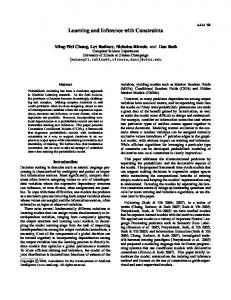
Figure 4: Functional phylogenetic tree for H. sapiens, M. musculus, S. cerevisiae, A. thaliana and E. coli in the Molecular Function and Cellular Component ontologies.

Figure 5: Functional phylogenetic tree for H. sapiens, M. musculus, S. cerevisiae, A. thaliana and E. coli in the Biological Process Ontology.

organisms X and Z, d(X, Z), was determined as an average between two directional distances; i.e., d(X, Z) = 21 · (dXZ + dZX ). It is worth further emphasizing that the sampling procedure in Algorithm 1 was chosen to reduce the influence of incomplete organismal annotations and large differences between available sets functions among organisms. For example, nE = 2272, nH = 11979 and nM = 6728 in MFO, which might cause a human protein to always be closer to any E. coli protein than any mouse protein, only because of a larger probability of a random close match, when in reality these two organisms are similarly distant from E. coli. The incomplete and biased annotations present a problem for creating functional phylogenies that is markedly different from clustering sets of sequence data, where the entire sequence complement for an organism is usually known and only sequences present in all species are used. 4.1.3

Functional Phylogenies

The entirety of the genetic information present within the model organisms considered here has been obtained, and the analysis of this genetic data has resulted in a well accepted set of phylogenetic relationships among these species. Using the distance measure introduced here, we generated functional phylogenies describing the relationships among these species using only protein function information. If our distance measure works well for the Gene Ontology data, we expect to recover the correct phylogenetic relationships. Using the MFO and CCO functional annotations our clustering approach did recover the correct relationships among species (Figure 4). This result is gratifying, especially as we might expect many similar functions to be present in the single-celled organisms (E. coli and S. cerevisiae). However, using the BPO annotations did not result in the correct phylogeny, as the positions of S. cerevisiae and A. thaliana were reversed (Figure 5). The accuracy of the MFO and CCO annotations and the inaccuracy of the BPO annotations are consistent with the higher level of functional conservation for the MFO annotations [21], as greater conservation of function could result in more phylogenetic signal within this ontology. As a reminder, this algorithm only produces an unrooted topology among the species. It is up to the experimenters to root the tree with some expert knowledge, as we have done here. 13

It is important to mention several practical issues related to the steps used to generate the functional phylogeny. First, as the functional data are biased and incomplete, it was relatively surprising that the available annotations could (approximately) recover the correct phylogenetic tree. We believe that as the biological data improves in quality the functional phylogeny should result in nearly identical results as the genetic sequence phylogeny, or perhaps may even be able to offer additional evolutionary insights [31]. This particularly holds for the BPO annotations that are of relatively lower quality and are also less predictable from sequence and molecular data [24]. Second, the choice of a clustering algorithm may affect the outcome of the phylogenetic reconstruction. Nonetheless, we experimented with clustering using single linkage, complete linkage, and group-average strategies for computing distances between clusters. We noticed little change in the resulting phylogenies for either ontology. There was also no dependence on the selection of N , where we evaluated N = 500, N = 1000, and N = 1500 (note that N was required to be smaller than the smallest term in Table 1).

5

Discussion

In this work we introduced new metrics on sets, ontologies, and functions that can be used in several stages of data processing pipelines, including supervised and unsupervised learning, exploratory data analysis, visualization, and result interpretation. We showed that these metrics are applicable on the space of protein functional annotations and that they have natural information-theoretic interpretation. Our experiments have revealed that our metrics can be used to correctly recover the phylogenetic relationships among species using only protein functions, and that they therefore represent promising measures for future studies of the evolution of function. In several recent publications, including our own, non-metric similarity functions have been used to reason about functional similarity between biological macromolecules as well as prediction accuracy of automated annotation tools. Assuming non-empty sets A and B, these include the Maryland bridge distance 

dMB (A, B) = 1 −

1 |A ∩ B| 1 |A ∩ B| + 2 |A| 2 |B|



where the term in the parentheses corresponds to the the Maryland bridge coefficient [8]. When A is interpreted as a predicted set of terms for a protein and B as a true set of terms, the Maryland bridge coefficient is simply an average of precision (|A∩B|/|A|) and recall (|A∩B|/|B|). Similarly, an often-used harmonic mean between precision and recall, referred to as F-measure [29], leads only to a near-metric called the Czekanowsky-Dice distance [6]. This distance function can be expressed as  −1 1 |A| 1 |B| dCD (A, B) = 1 − + 2 |A ∩ B| 2 |A ∩ B| where, again, A and B are sets and the second term on the right-hand side is the F-measure. While on the surface the process of finding an average pairwise distance for a set of graphs appears to be straightforward, it is unclear what the effect of such operations might be when the concept of triangle inequality is violated. We therefore caution the interpretation of results when non-metric distance functions are used. Although our experimental investigation only considered biomedical ontologies, the metrics proposed in Equations (1)-(6) have broader applicability. For example, metrics on ontologies can be directly used in the areas of text mining or computer vision in the tasks of joint topic classification [9] or fine-grained classification [20]. Alternatively, the continuous versions might be readily applicable 14

in comparisons of probability distributions as an alternative to Kullback-Leibler divergence [14] that lacks theoretical properties such as symmetry and triangle inequality (the symmetry requirement can be remedied by using the J-divergence [16]). Finally, we emphasize that it is difficult to empirically demonstrate that a particular metric is useful in any setting since a common practice in modeling is to initially select an objective function based on domain knowledge and then to develop an algorithm to directly minimize it. Therefore, we believe that the class of functions proposed in this work present sensible choices in various fields and hope that their good theoretical properties will play a positive role in their adoption.

A

Appendix

Lemma A.1. For any real functions f , g we have f + + g + = min(|f |, |g|)1{f g 0, then we have ( +

+

+

+

f + g − (f + g) = g − (f + g) =

g, if |f | > |g| = min(|f |, |g|). −f, if |f | ≤ |g|

Lemma A.2. For any real functions f, g and h, we have (f − g)+ + (g − h)+ − {max(|g|, |f − g|, |g − h|) − max(|f |, |h|, |f − h|)}+ ≥ (f − h)+ .

Proof. By Lemma A.1, it is equivalent to show min(|f − g|, |g − h|)1{(f −g)(g−h) 0, pick n to be N0 and we have 1

(( (fN0 − fm )− dx)p + ( (fN0 − fm )+ dx)p ) p R DN (fN0 , fm ) = |fm | + |fN0 |) dx R

Z

R

−

Z

1

= (( (Am − Bm ) dx) + ( (Am − Bm )+ dx)p ) p where Am = R

fN0 , |fm | + |fN0 |) dx

p

Bm = R 16

fm |fm | + |fN0 |) dx

and {Am } and {BmR} are sequences of functions. Fixing N0 and sending n to ∞ we have that R |Am | dx → 0 and R|Bm | dx → 1 as m → ∞. Therefore, we could choose m > N0 such that R R − R + |Am | dx < 1/10 and |Bm | dx > 9/10. Then betweenR Bm dx and Bm dx there is at least one − dx > 9/20, then greater than 9/20. Without loss of generality, suppose Bm Z

1

DN (fN0 , fm ) ≥ ( (Am − Bm )+ dx)p ) p Z

= ≥ ≥ >

Z Z

(Bm − Am )− dx −

Z

(Bm )− dx −

Z

(Bm ) dx −

(Am )− dx |Am | dx

7 20

With this we have shown that for any N0 > 0, there exist m, n ≥ N0 such that DN (fn , fm ) > 7/20; i.e., {fn } is not a Cauchy sequence in (L(R), DN ). Thus, we have proved the claim.

Acknowledgements This work was partially supported by the NSF grants DBI-1458477 (PR) and DMS-1206405 (EAH). We thank Jovana Kovaˇcevi´c for helpful discussions and Henry Horton for technical assistance.

References [1]

M. Ashburner et al. “Gene ontology: tool for the unification of biology. The Gene Ontology Consortium”. In: Nat Genet 25.1 (2000), pp. 25–29.

[2]

A. Bairoch et al. “The Universal Protein Resource (UniProt)”. In: Nucleic Acids Res 33.Database issue (2005), pp. D154–159.

[3]

S. Baraty et al. “The impact of triangular inequality violations on medoid-based clustering”. In: Foundations of Intelligent Systems. Springer, 2011, pp. 280–289.

[4]

S. Ben-David and M. Ackerman. “Measures of clustering quality: A working set of axioms for clustering”. In: Adv Neural Inf Process Syst. 2009, pp. 121–128.

[5]

W. T. Clark and P. Radivojac. “Information-theoretic evaluation of predicted ontological annotations”. In: Bioinformatics 29.13 (2013), pp. i53–i61.

[6]

M. M. Deza and E. Deza. Encyclopedia of distances. Springer, 2013.

[7]

C. Elkan. “Using the triangle inequality to accelerate k-means”. In: Proc 20th Int Conf Mach Learn. 2003, pp. 147–153.

[8]

G. Glazko, A. Gordon, and A. Mushegian. “The choice of optimal distance measure in genomewide datasets”. In: Bioinformatics 21.Suppl 3 (2005), pp. iii3–iii11.

[9]

M. Grosshans et al. “Joint prediction of topics in a URL hierarchy”. In: Proceedings of the European Conference on Machine Learning and Principles and Practice of Knowledge Discovery in Databases. ECML/PKDD 2014. Nancy, France, 2014, pp. 514–529. 17

[10]

P. H. Guzzi et al. “Semantic similarity analysis of protein data: assessment with biological features and issues”. In: Brief Bioinform 13.5 (2012), pp. 569–585.

[11]

J. J. Jiang and D. W. Conrath. “Semantic similarity based on corpus statistics and lexical taxonomy”. In: Proc Int Conf Res Computational Linguistics. 1997, pp. 19–33.

[12]

Y. Jiang et al. “The impact of incomplete knowledge on the evaluation of protein function prediction: a structured-output learning perspective”. In: Bioinformatics 30.17 (2014), pp. i609– i616.

[13]

M. Kryszkiewicz and P. Lasek. “TI-DBSCAN: clustering with DBSCAN by means of the triangle inequality”. In: Rough Sets and Current Trends in Computing. Springer. 2010, pp. 60– 69.

[14]

S. Kullback and R. A. Leibler. “On information and sufficiency”. In: Ann Math Stat 22.1 (1951), pp. 79–86.

[15]

D. Lin. “An information-theoretic definition of similarity”. In: Proc 15th Int Conf Mach Learn. 1998, pp. 296–304.

[16]

J. Lin. “Divergence measures based on the Shannon entropy”. In: IEEE Trans Inform Theory 37.1 (1991), pp. 145–151.

[17]

P. W. Lord et al. “Investigating semantic similarity measures across the Gene Ontology: the relationship between sequence and annotation”. In: Bioinformatics 19.10 (2003), pp. 1275– 1283.

[18]

E. Marczewski and H. Steinhaus. “On a certain distance of sets and the corresponding distance of functions”. In: Colloquium Mathematicae. Vol. 6. 1. 1958, pp. 319–327.

[19]

G. K. Mazandu and N. J. Mulder. “A topology-based metric for measuring term similarity in the gene ontology”. In: Adv Bioinformatics (2012), p. 975783.

[20]

Y. Movshovitz-Attias et al. “Ontological supervision for fine grained classification of street view storefronts”. In: IEEE Conference on Computer Vision and Pattern Recognition. CVPR 2015. 2015, pp. 1693–1702.

[21]

N. L. Nehrt et al. “Testing the ortholog conjecture with comparative functional genomic data from mammals”. In: PLoS Comput Biol 7.6 (2011), e1002073.

[22]

C. Pesquita et al. “Semantic similarity in biomedical ontologies”. In: PLoS Comput Biol 5.7 (2009), e1000443.

[23]

R. Rada et al. “Development and application of a metric on semantic nets”. In: IEEE Trans Syst Man Cybern 19.1 (1989), pp. 17–30.

[24]

P. Radivojac et al. “A large-scale evaluation of computational protein function prediction”. In: Nat Methods 10.3 (2013), pp. 221–227.

[25]

P. Resnik. “Semantic similarity in a taxonomy: an information-based measure and its application to problems of ambiguity in natural language”. In: J Artif Intell Res 11 (1999), pp. 95–130.

[26]

P. Resnik. “Using information content to evaluate semantic similarity in a taxonomy”. In: Proc 14th Int Joint Conf Artif Intell. 1995, pp. 448–453.

[27]

P. N. Robinson and S. Bauer. Introduction to bio-ontologies. Boca Raton, Florida, U.S.A.: CRC Press, 2011.

18

[28]

A. Schlicker et al. “A new measure for functional similarity of gene products based on Gene Ontology”. In: BMC Bioinformatics 7 (2006), p. 302.

[29]

P. N. Tan, M. Steinbach, and V. Kumar. Introduction to data mining. Boston, MA: Pearson Education, Inc., 2006.

[30]

K. Verspoor et al. “A categorization approach to automated ontological function annotation”. In: Protein Sci 15.6 (2006), pp. 1544–1549.

[31]

C. Zhu et al. “Functional basis of microorganism classification”. In: PLoS Comput Biol 11.8 (2015), e1004472.

19