Use of Radial Basis Functions and Rough Sets for Evolutionary Multi-Objective Optimization Luis V. Santana-Quintero1, V´ıctor A. Serrano-Hern´andez 1 Carlos A. Coello Coello1 , Alfredo G. Hern´andez-D´ıaz2 and Juli´an Molina3 1
CINVESTAV-IPN (Evolutionary Computation Group) ´ Computer Science Department, MEXICO 2 Dept. of Quantitative Methods, Pablo de Olavide University, SPAIN 3 Dept. of Applied Economics (Mathematics), University of M´alaga, SPAIN
[email protected],
[email protected] [email protected],
[email protected] [email protected] Abstract— This paper presents a new multi-objective evolutionary algorithm (MOEA) which adopts a radial basis function (RBF) approach in order to reduce the number of fitness function evaluations performed to reach the Pareto front. The specific method adopted is derived from a comparative study conducted among several RBFs. In all cases, the NSGA-II (which is an approach representative of the state-of-the-art in the area) is adopted as our search engine with which the RBFs are hybridized. The resulting algorithm can produce very reasonable approximations of the true Pareto front with a very low number of evaluations, but is not able to spread solutions in an appropriate manner. This led us to introduce a second stage to the algorithm in which it is hybridized with rough sets theory in order to improve the spread of solutions. Rough sets, in this case, act as a local search approach which is able to generate solutions in the neighborhood of the few nondominated solutions previously generated. We show that our proposed hybrid approach only requires 2,000 fitness function evaluations in order to solve test problems with up to 30 decision variables. This is a very low value when compared with today’s standards reported in the specialized literature.
I. I NTRODUCTION Multi-objective optimization problems are of great importance, since they are very common in a wide variety of disciplines. Multi-objective problems have two or more objectives which are normally in conflict with each other. Therefore, instead of having a single solution, they normally have a set of solutions (called the Pareto optimal set) all of which are equally good among themselves. Despite the existence of a variety of mathematical programming techniques to solve multi-objective optimization problems, the use of evolutionary algorithms in this area has become very popular in the last few years [1], [2], mainly because of their ease of use, and their wide applicability. However, despite their several advantages, multi-objective evolutionary algorithms (MOEAs) tend to require an important number of objective function evaluations, in order to achieve a reasonably good approximation of the Pareto front, even when dealing with benchmark problems of low dimensionality. This issue becomes critical when attempting to solve real-world problems in which we can only afford performing a very low number of fitness function evaluations. It has been only until
recently that researchers have started to develop MOEAs that perform a very low number of fitness function evaluations. The purpose of this paper is precisely to introduce a new hybrid approach which combines a MOEA with RBFs in order to produce a quick (i.e., with a low number of fitness function evaluations) approximation of the Pareto front. Then, rough sets are used to diversify the neighborhood surrounding each of the nondominated solutions produced with this hybrid MOEA, such that the rest of the Pareto front is reconstructed. The remainder of this paper is organized as follows. Section II provides the required background for the use of Radial Basis Functions to approximate a function. In Section III, we provide a brief introduction to rough sets theory and a quick review of the most relevant previous related work is described in Section IV. Section V describes our proposed approach. Our comparison of results is provided in Section VI. Finally, in Section VII, we provide some of the paths for future research and the conclusions of this work. II. F ITNESS A PPROXIMATION
USING
RBF S
RBFs were first introduced by R. Hardy in 1971 [4]. This term is made up of two different words: radial and basis functions. A radial function refers to a function of the type: g : Rd → R : (x1 , . . . , xd ) 7→ φ(kx1 , . . . , xd k2 ) for some function φ : R → R. This means that the function → value of g at a point − x = (x1 , . . . , xd ) only depends on the − → Euclidean norm of x : v u d uX − → → kxk = t x to the origin x2 = distance of − 2
i
i=0
And this explains the term radial. The term basis function is explained next. Let’s suppose we have certain points (called → → centers) − x 1, . . . , − x n ∈ Rd . The linear combination of the → function g centered at the points − x is given by: → f : Rd 7→ R : − x 7→
n X i=1
→ → λi g(− x −− xi ) =
n X i=1
→ → λi φ(k− x −− xi k) (1)
Type of Radial Function LS TPS CS MQS GA
linear splines thin plate splines cubic splines multiquadrics splines Gaussian
|r| |r|2m+1 ln |r| 3 p |r| 1 + (ǫr)2 2 e−(ǫr)
TABLE I R ADIAL BASIS F UNCTIONS
→ → where k− x −− xi k is the Euclidean distance between the → → points − x and − x i . So, f becomes a function which is in the finite dimensional space spanned by the basis functions: → → → gi : − x → 7 g(k− x −− xi k)
Density(G) =
Now, let us suppose that we already know the values of a certain function H : Rd 7→ R at a set of fixed locations − → − → xi , . . . , − x→ n . These values are named fj = H(xj ), so we try − → to use the xj as centers in equation (1). If we want to force → the function f to take the values fj at the different points − xj , then we have to put some conditions on the λi . This implies the following: − →j ) = ∀j ∈ {1, . . . , n} fj = f (x
n X
− →j − − → (λi · φ(kx xi k))
i=1
In these equations, only the λi are unknown, and the equations are linear in their unknowns. Therefore, we can write these equations in matrix form: 2 6 6 6 6 6 4
φ(0) φ(kx2 − x1 k) . . . φ(kxn − x1 k)
φ(kx1 − x2 k) φ(0) . . . φ(kxn − x2 k)
... ...
...
3 2 φ(kx1 − xn k) φ(kx2 − xn k) 7 6 7 6 7 6 . 7·6 7 6 . 5 4 . φ(0)
(probably) inside X if it belongs to the upper approximation. The boundary is the difference of these two sets, and the bigger the boundary the worse the knowledge we have of set X. On the other hand, the more precise is the grid implicity used to define the indiscernibility relation R, the smaller the boundary regions are. But, the more precise is the grid, the bigger the number of elements in U , and then, the more complex the problem becomes. Consequently, the goal is obtaining “small” grids with the maximum precision possible. These two aspects are called Density and Quality of the grid. If q is the number of criteria (in our case, the number of objectives), Qi is the i-th criterion, bij is the j-th value of the i-th criterion (we assume these values are ordered increasingly), then:
λ1 λ2 . . . λn
3
2
7 6 7 6 7 6 7 =6 7 6 5 4
f1 f2 . . . fn
3 7 7 7 7 7 5 (2)
→ Typical choices for the basis functions g(− x ) include linear splines, cubic splines, multiquadrics, thin-plate splines and Gaussian functions as shown in Table I. III. ROUGH S ETS T HEORY Rough sets theory was proposed by Pawlak [11] as a new mathematical approach to imperfect knowledge. The basics of this approach are briefly described next. Let us assume that we are given a set of objects U called the universe and an indiscernibility relation R ⊆ U × U , representing our lack of knowledge about elements of U (in our case, R is simply an equivalence relation based on a grid over the feasible set; this is, just a division of the feasible set in (hyper)-rectangles). Let X be a subset of U . We want to characterize the set X with respect to R. The way rough sets theory expresses vagueness is employing a boundary region of the set X built once we know points both inside X and outside X. If the boundary region of a set is empty it means that the set is crisp; otherwise, the set is rough (inexact). A nonempty boundary region of a set means that our knowledge about the set is not enough to define the set precisely. Then, each element in U is classified as certainly inside X if it belongs to the lower approximation or partially
|Qi | q X X
xij
i=1 j=1
Quality(G) =
|Low(X)| |X|
where xij is 1 if bij is active in the grid and |Low(X)| is the cardinality of the lower approximation of X. IV. P REVIOUS R ELATED W ORK Currently, there exist several evolutionary algorithms that use a meta-model to approximate the real fitness function and reduce the total number of fitness evaluations without degrading the quality of the results obtained. Note however, that very few of these approaches are multi-objective. Next, we will briefly review the most significant work in this area. Various approximation levels or strategies adopted for fitness approximation in evolutionary computation are proposed in [6]. Ong et al. [10] used surrogate models (RBFs) to solve computationally expensive design problems with constraints. The authors used a parallel evolutionary algorithm coupled with sequential quadratic programming in order to find optimal solutions of an aircraft wing design problem. In this case, the authors construct a local surrogate model based on radial basis functions in order to approximate the objective and constraint functions of the problem. Karakasis et al. [7] used surrogate models based on radial basis functions in order to deal with computationally expensive problems. A method called Inexact Pre-Evaluation (IPE) is applied into a MOEA’s selection mechanism. Such method helps to choose the individuals that are to be evaluated using the real objective function, right after a meta-model approximation has been obtained by the surrogate. The results are compared against a conventional MOEA in two test problems, one from a benchmark and one from the turbomachinery field. Voutchkov & Keane [5] studied several surrogate models (RSM, RBF and Kriging) in the context of multi-objective optimization using the NSGAII [3] as the MOEA that optimized the meta-model function given by the surrogate. The surrogate model is trained with 20 initial points and the NSGA-II is run on the surrogate model. Then, the 20 best resultant points given by the optimization are added to the existing data pool of real function evaluations and the surrogate is re-trained with these new solutions. A
comparison of results is made in 4 test functions (from 2 to 10 variables), performing only 400 real fitness function evaluations. Knowles [8] proposed “ParEGO”, which consists of a hybrid algorithm based on a single optimization model (EGO) and a Gaussian process, which is updated after every function evaluation, coupled to an evolutionary algorithm. EGO is a single-objective optimization algorithm that uses Kriging to model the search landscape from the solutions visited during the search and learns a model based on Gaussian processes (called DACE). This approach is used to solve multiobjective optimization problems of low dimensionality (up to 6 decision variables) with only 100 and 250 fitness function evaluations. V. P ROPOSED A PPROACH Our proposed approach, is divided in two different phases, and each of them consumes a fixed number of fitness function evaluations. In the first phase, our surrogate-based MOEA is applied for 1000 fitness function evaluations. However, since several RBFs exist, we decided to perform a comparative study among several of them, in order to determine which one is the most appropriate for our purposes. The results of this comparative analysis are discussed in Section VI. The results obtained from the first phase led us to conclude that a local search mechanism was necessary in order to spread the nondominated solutions previously found, such that a much better approximation of the entire Pareto front could be achieved. Thus, the second phase of our algorithm consists of applying rough sets theory for 1,000 fitness function evaluations in order to improve the solutions produced during the first phase. A. RBFs-based MOEA The RBFs-model adopted in our approach is shown in Figure 1. As can be seen, the NSGA-II [3] is used to optimize the approximated model generated by the RBFs. Our approach keeps two populations: the main population (which is used to select the parents) and a secondary population, that retains dominated solutions found during the evolutionary process (this secondary population is needed by the second phase that uses rough sets). First, we generate P individuals using Latin-Hypercubes [9], which is a method that guarantees a good distribution of the initial population in a multidimensional space. If we do a simple random sampling of the initial points, where the new sample points are generated without taking into account the previously generated sample points, we may not be able to obtain points in some critical areas from the search space. Our approximation model requires a good distribution of the sample points provided, in order to build a good approximation of the real functions and therefore the importance of adopting this approach. A Latin cube is a selection of one point from each row and column of a square matrix. In M dimensions, the corresponding item is a set of P points, where, in each dimension, there is exactly one point per column or range
of values. In M dimensions, these objects are called LatinHypercubes. Once a Latin-Hypercube has been created, we choose the center of each hypercube as the place where the initial P individuals are chosen. Then, we evaluate these P individuals with the real objective functions, and train the meta-model using the RBFs. As we are dealing with multiobjective problems, we decided to train the multiple objectives separately. Consequently, we obtain a different RBF per each objective, so these objectives are still in conflict with each other as they are an approximate model of the real objectives. Thus, we now have to solve a different multi-objective problem based on the different RBF obtained during the training process. We use the NSGA-II [3], which adopts a fast nondominated sorting approach to classify solutions according to levels of nondomination and a crowding distance operator, which is responsible for preserving diversity. The NSGA-II is adopted to optimize the meta-model obtained by the RBFs. From all the nondominated solutions found by the NSGA-II, we decided to retain only 20 points. These new points obtained by the NSGA-II are compared with respect to all the points in the main population and those that are different with respect to all the points contained in the main population are accepted and evaluated using the real objective function values. All the solutions contained in the main population are used to re-train the meta-model (using RBFs) and get another approximation of the real objectives. As it is shown in Figure 1, this procedure is repeated until the number of M axEval evaluations is fulfilled. With this procedure, the size of the main population is increased as the real objective function evaluations are performed. As the main population becomes larger, the training process takes more computational time to do the approximation because the Φ matrix is larger and the matrix inversion process takes more and more time. So, we decided to accept a maximum of 500 solutions in the main population. When this number is reached, we choose only the 300 best solutions (based on rank & crowding distance sorting) to continue with the training process. At the end of the procedure, we select 52 nondominated solutions from the main population, and we store 100 dominated solutions in the secondary population, which stores the dominated points needed for the Phase II. Every removed point from the main population is included in the secondary population. If this secondary population reaches a size of 100 points, a rank and crowding distance sorting is used to keep only 100 points (the remainder are eliminated). B. Phase 2: Rough Sets in Multi-Objective Optimization For our MOPs we will try to approximate the Pareto front using a rough sets grid. To do this, we will use an initial approximation of the Pareto front (provided by the main population obtained from the first phase previously described) and we implement a grid in order to get more information about the front which allow us to improve this initial approximation. As indicated before, we need to design a grid that is not so expensive (computationally speaking) but that offers a
Fig. 1.
RBFs algorithm, which uses the NSGA-II to optimize the meta-model.
to create it, we will try to use just a few points. However, such points must be as far from each other as possible, because the better the distribution the points have in the initial approximation the less points we need to build a reliable grid. On the other hand, in order to diversify the search we build several grids using different (and disjoint) sets DS and ES coming from the initial approximation. To ensure these sets are really disjoint we will mark each point as explored or non-explored (i.e., we distinguish if it has been used or not to compute a grid) and we will not allow repetitions. Algorithm 1 describes a Rough Sets iteration. Fig. 2.
Decision variable space (left) and objective function space (right)
Algorithm 1 Rough Sets Iteration reasonably good knowledge about the Pareto front to be used to improve the initial approximation. To this aim, we have to decide which elements of U (that we will call atoms and are rectangular portions of decision variable space) are inside the Pareto optimal set and which are not. Once we have the efficient atoms, we can easily intensify the search over these atoms as they are built in decision variable space. To create this grid, as an input we will have N feasible points divided in two sets: the nondominated points (ES) and the dominated ones (DS). Using these two sets we want to create a grid to describe the set ES in order to intensify the search on it. This is, we want to describe the Pareto front in decision variable space because then we could easily use this information to generate more efficient points and then improve this initial approximation. Figure 2 shows how information in objective function space can be translated into information in decision variable space through the use of a grid. We must note the importance of the DS set since in a rough sets method the information comes from the description of the boundary of the two sets. Then, the more efficient points provided the better. However, it is also required to provide dominated points, since we need to estimate the boundary between being dominated and being nondominated. Once this information is computed, we can simply generate more points in the “efficient side”. Since the computational cost of managing the grid increases with the number of points used
1: 2: 3: 4: 5: 6: 7: 8: 9: 10: 11: 12: 13: 14: 15: 16: 17:
Choose N umEf f non-explored points of ES. Choose N umDom non-explored points of DS. Generate N umEf f efficient atoms. for i = 0 to N umEf f do for j = 0 to Of f spring do Generate (randomly) a point new in atom i and send to ES if new is efficient then Include in ES end if if A point old in ES is dominated by new then Send old to DS end if if new is dominated by a point in ES then Remove new end if end for end for
VI. D ISCUSSION AND R ESULTS As we have mentioned, our main goal is to reduce the number of fitness function evaluations. Thus, our experimental design considers that only a few function evaluations are performed in several multi-dimensional test problems from the ZDT set [13]. The detailed description of these test functions was omitted due to space restrictions (see [13] for further information). However, all of these test functions are biobjective, unconstrained minimization problems and have between 10 and 30 decision variables. Three performance measures were adopted in order to allow a quantitative assessment of our results: (1) Inverted Generational Distance (IGD), which is a variation of a metric proposed by Van Veldhuizen [12]
in which the true Pareto is used as a reference; (2) Two Set Coverage (SC), proposed by Zitzler et al. [13], which performs a relative coverage comparison of two sets; and (3) Spread (S), proposed by Deb et al. [2], which measures both progress towards the Pareto-optimal front and the extent of spread. For each test problem, 30 independent runs were performed. This section is divided in two parts: in the first one, we compare the results obtained by the surrogate-based NSGA-II with respect to the original NSGA-II. Both approaches perform 1,000 real function evaluations in this case. In the second part, the Rough Sets Theory algorithm is applied for another 1,000 real function evaluations and the results are compared with respect to the original NSGA-II performing 2,000 evaluations.
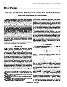
ZDT1 pareto front 5
LRBF TPRBF 4
CRBF MQRBF GRBF
Function 2
3
TPRBF 2
LRBF NSGA-II
1
CRBF MQRBF GRBF
0
0.0
A. First Phase Analysis The first phase of our approach uses several parameters: main population size (P = 20), internal NSGA-II population size (Pnsga2 = 52), internal NSGA-II maximum number of generations (Gnsga2 = 50), crossover rate = 0.9, mutation rate = 1/n (n = number of decision variables), ηc = 15, ηm = 20. The NSGA-II used the following parameters: crossover rate = 0.9, mutation rate = 1/n, ηc = 15, ηm = 20, population size = 52 and maximum number of generations = 20. In this study, we perform 1,000 real function evaluations using different RBFs: Linear (LRBF), Thin Plate (TPRBF), cubic (CRBF), multiquadrics (MQRBF) and Gaussian (GRBF). They are all compared to the original NSGA-II. The results reported in Table II correspond to the mean and standard deviation (σ) of the performance metrics (IGD, SC and S). We show in boldface the best mean values per test function of 30 runs per each test function by all algorithms. We show the plot of all the nondominated solutions generated by a single run of the different algorithms in Figures 3, 4 and 5. In all cases, we generated the P Ftrue of the problems using exhaustive enumeration so that we could make a graphical comparison of the quality of the solutions produced by our approach. • LRBF: Using the Linear Radial Basis Function, the algorithm shows a poor performance dealing with highdimensional problems. The NSGA-II outperforms this approach in all cases except for ZDT1. Graphically, it can be observed that in all the plots the NSGA-II is closer to the true Pareto front than the LRBF. • TPRBF: With Thin Plate Splines, the algorithm shows the worst performance of the variants studied in this paper. With respect to the performance measures adopted, in all cases TPRBF is outperformed by the NSGA-II and graphically, it can be seen that this approach never reaches the true Pareto front and stays far away from the other techniques. • CRBF: Using the Cubic function, the algorithm outperformed the NSGA-II only in ZDT1, ZDT2 and ZDT6. With respect to the Spread metric, it can be shown that the results are very poor. The NSGA-II gets better results than CRBF in Spread in almost all the functions except for ZDT6 (in which the difference is very low). Graphically, the performance of the CRBF is almost the same in all the
NSGA-II
0.2
0.4
0.6
0.8
1.0
Function 1
Fig. 3.
Pareto fronts generated by RBFs variants and NSGA-II for ZDT1
test functions as that obtained with the NSGA-II. None of the approaches was able to reach the true Pareto Front. • MQRBF: Using a Multiquadric function, the results shown in Table II are quite competitive with respect to the NSGA-II in almost all the ZDTs functions, except for ZDT4 in which MQRBF shows a poor performance. In Figure 5(a), it can be seen that in ZDT4, MQRBF is far away from the true Pareto front and from the results obtained by the NSGA-II. • GRBF: With the Gaussian RBF, the algorithm shows the best performance of all the variants, regarding all the performance measures. GRBF gets the best results in ZDT1, ZDT2 and ZDT6 from all the variants compared and also outperforms the NSGA-II. In ZDT3 and ZDT4, the NSGA-II outperforms GRBF. Graphically, GRBF is the most competitive method in all cases, showing a good aproximation to the real Pareto Front in ZDT1, and in the other test functions, it obtains a reasonably good approximation. We can conclude from the results shown in Table III that the GRBF algorithm is the one that shows the best overall performance in these particular multi-dimensional test functions. So, in the second phase of our analysis, we extend the solutions generated by the GRBF model and we show the performance of the algorithm when it is hybridized with rough sets theory. B. Second Phase Analysis If we pay particular attention to the plots shown in Figures 3, 4 and 5, corresponding to all the RBFs, it can be seen that they only get a few solutions on the Pareto front. So, clearly convergence is achieved at the expense of sacrificing spread of solutions along the Pareto front. This led us to think that if we incorporated a local search method such as the rough sets theory, we could fill up the holes (gaps) and find the solutions that are missing in these Pareto sets. So, we decided to perform
IGD SURROGATE NSGA-II Mean σ Mean σ 0.10288 0.03272 0.20800 0.03104 0.69647 0.08921 0.20800 0.03104 0.11771 0.20930 0.20800 0.03104 0.04180 0.04852 0.20800 0.03104 0.01897 0.06016 0.20800 0.03104 0.81028 0.13745 0.46775 0.08492 1.22407 0.15678 0.46775 0.08492 0.42130 0.27687 0.46775 0.08492 0.17984 0.26638 0.46775 0.08492 0.10576 0.16785 0.46775 0.08492 0.20736 0.04469 0.18475 0.03819 0.62043 0.10131 0.18475 0.03819 0.24337 0.1551 0.18475 0.03819 0.20586 0.08155 0.18475 0.03819 0.26424 0.10398 0.18475 0.03819 15.17009 5.51475 12.34834 3.47526 24.62728 6.10294 12.34834 3.47526 29.54019 6.04672 12.34834 3.47526 32.53860 7.58354 12.34834 3.47526 18.56345 4.81500 12.34834 3.47526 1.58455 0.41908 1.40626 0.20648 2.43238 0.29497 1.40626 0.20648 1.28818 0.68509 1.40626 0.20648 0.58939 0.20367 1.40626 0.20648 0.51180 0.13866 1.40626 0.20648
Function ZDT1 (LRBF) ZDT1 (TPRBF) ZDT1 (CRBF) ZDT1 (MQRBF) ZDT1 (GRBF) ZDT2 (LRBF) ZDT2 (TPRBF) ZDT2 (CRBF) ZDT2 (MQRBF) ZDT2 (GRBF) ZDT3 (LRBF) ZDT3 (TPRBF) ZDT3 (CRBF) ZDT3 (MQRBF) ZDT3 (GRBF) ZDT4 (LRBF) ZDT4 (TPRBF) ZDT4 (CRBF) ZDT4 (MQRBF) ZDT4 (GRBF) ZDT6 (LRBF) ZDT6 (TPRBF) ZDT6 (CRBF) ZDT6 (MQRBF) ZDT6 (GRBF)
Set Coverage SURROGATE NSGA-II Mean σ Mean σ 0.23604 0.34404 0.69013 0.37920 1.00000 0.00000 0.00000 0.00000 0.16837 0.32175 0.78346 0.39462 0.00526 0.02834 0.98805 0.05761 0.03066 0.16514 0.96666 0.17950 0.32425 0.30095 0.01587 0.04487 1.00000 0.00000 0.00000 0.00000 0.27473 0.32160 0.52686 0.41170 0.11527 0.29924 0.81726 0.35576 0.01333 0.04988 0.94326 0.18007 0.96288 0.02922 0.00418 0.01684 0.99791 0.01121 0.00000 0.00000 0.31808 0.39346 0.58778 0.43849 0.29712 0.33232 0.58882 0.38307 0.55617 0.37069 0.29089 0.38190 0.28802 0.30796 0.46673 0.33417 0.95417 0.08144 0.02198 0.05112 0.76380 0.24553 0.03269 0.10027 0.71297 0.23332 0.02190 0.05226 0.34171 0.33166 0.41920 0.33087 0.97790 0.06191 0.00000 0.00000 1.00000 0.00000 0.00000 0.00000 0.45890 0.41739 0.33283 0.29411 0.02484 0.09983 0.70901 0.30467 0.00333 0.01795 0.76644 0.27833
Spread SURROGATE NSGA-II Mean σ Mean σ 0.66046 0.05919 0.74052 0.06068 0.82493 0.04287 0.74052 0.06068 0.56614 0.16527 0.74052 0.06068 0.57483 0.09978 0.74052 0.06068 0.48263 0.09297 0.74052 0.06068 0.89139 0.06925 0.89369 0.06795 0.89555 0.04259 0.89369 0.06795 0.80797 0.14153 0.89369 0.06795 0.66155 0.22242 0.89369 0.06795 0.65771 0.20612 0.89369 0.06795 0.84313 0.02779 0.76863 0.05741 0.84909 0.05301 0.76863 0.05741 0.74887 0.10645 0.76863 0.05741 0.76560 0.07593 0.76863 0.05741 0.79371 0.05849 0.76863 0.05741 0.98826 0.00945 0.98714 0.01113 0.99180 0.00297 0.98714 0.01113 0.99524 0.00311 0.98714 0.01113 0.99533 0.00260 0.98714 0.01113 0.99136 0.00584 0.98714 0.01113 0.94045 0.03465 0.92336 0.04662 0.91622 0.03926 0.92336 0.04662 0.89442 0.05776 0.92336 0.04662 0.88068 0.09220 0.92336 0.04662 0.85790 0.04349 0.92336 0.04662
TABLE II C OMPARISON OF RESULTS BETWEEN RBF S ALGORITHM AND THE NSGA-II (1000 EVALUATIONS ).
ZDT2 pareto front 5
ZDT3 pareto front
NSGA-II
NSGA-II
LRBF
LRBF
5
TPRBF
TPRBF
TPRBF
CRBF
4
CRBF 4
MQRBF
MQRBF
GRBF
GRBF
LRBF
3
NSGA-II 2
CRBF GRBF
Function 2
Function 2
3
2
TPRBF LRBF
1
GRBF
MQRBF
NSGA-II
1
CRBF 0
0
MQRBF
-1
0.0
0.2
0.4
0.6
0.8
1.0
Function 1
(a) ZDT2 Fig. 4.
0.0
0.2
0.4
0.6
0.8
1.0
Function 1
(b) ZDT3
Pareto fronts generated by RBFs variants and NSGA-II for ZDT2 and ZDT3 test functions.
1,000 more fitness function evaluations, aiming to fill up the gaps along the Pareto front. The second phase uses three more parameters: number of points randomly generated inside each atom (Of f spring), number of atoms per generations (N umEf f ) and the number of dominated points considered to generate the atoms (N umDom). Of f spring = 1, N umEf f = 2 and N umDom = 10. The NSGA-II used the same parameters described in the first analysis except for the maximum number of generations = 40 instead of 20
(used in the first analysis), so that the NSGA-II performs 2,000 fitness function evaluations in total. This will allow a fair comparison between both approaches. It can be observed that in the ZDTs test problems our approach produced the best results with respect to the SC metric in all cases. The same applies for the IGD metric, except for ZDT4. Also, our approach outperformed the NSGA-II with respect to the spread metric in three cases (ZDT1, ZDT2 and ZDT6). Graphically, it can be seen that our approach gets closer to the true Pareto
ZDT6 pareto front NSGA-II
ZDT4 pareto front 12
NSGA-II
180
LRBF TPRBF
LRBF
CRBF
TPRBF
160
10
CRBF 140
MQRBF GRBF
MQRBF GRBF
8
120
Function 2
Function 2
TPRBF 100
80
MQRBF
LRBF
6
NSGA-II 4
60
CRBF 40
MQRBF
CRBF
20
GRBF
2
LRBF
TPRBF
NSGA-II GRBF
0
0 0.0
0.2
0.4
0.6
0.8
1.0
Function 1
(a) ZDT4 Fig. 5.
0.2
0.4
0.6
0.8
1.0
Function 1
(b) ZDT6
Pareto fronts generated by RBFs variants and NSGA-II for ZDT4 and ZDT6 test functions.
front in ZDT1, ZDT2, ZDT3 and ZDT6, but not in ZDT4. The poor performance of all the approaches in ZDT4 might be attributed to the bad scalability presented by approaches based on genetic algorithms such as the NSGA-II. Our results indicate that the NSGA-II, despite being a highly competitive MOEA, is not able to converge to the true Pareto front in most of the test problems adopted when performing only 2,000 fitness function evaluations. If allowed a higher number of evaluations, the NSGA-II would certainly produce a very good (and well-distributed) approximation of the Pareto front. However, our aim was precisely to provide an alternative approach that could require a lower number of evaluations than a state-of-the-art MOEA while still providing a highly competitive performance. Such an approach could be useful in real-world applications with objective functions requiring a very high evaluation cost (computationally speaking). VII. C ONCLUSIONS AND F UTURE W ORK We have presented a Radial Basis Function approach to deal with multi-objective problems. The specific RBF adopted was derived from an empirical study in which several variants were compared when dealing with high dimensional test problems. From this study, we concluded that the Gaussian RBF was the most appropriate model for our needs. However, despite achieving a good convergence, this RBF cannot produce a good spread of solutions. Thus, we decided to include a local search procedure based on rough sets theory in order to intensify the search in the neighborhood of the solutions previously found by the RBF. This hybrid was found to provide very competitive results in most of the test problems adopted. These results, although preliminary, seem to indicate that our approach could be a viable alternative for real-world applications in which each evaluation of the fitness function is very
expensive (computationally speaking). In such applications, we can afford sacrificing a good distribution of solutions for the sake of obtaining a reasonably good approximation of the Pareto front with a low number of evaluations. As part of our future work, we are interested in refining the interaction mechanism between the RBF and the MOEA, such that the interleaving of these two approaches maximizes performance. We are also interested in experimenting with other approximation techniques such as artificial neural networks and Gaussian processes. We are also interested in studying the use of regression-based RBFs to improve the problem of data training overfitting when the number of data increases. ACKNOWLEDGMENT The first and second authors acknowledge support from CONACyT to pursue graduate studies at CINVESTAV’s Computer Science Department. The third author gratefully acknowledges support from CONACyT project no. 42435-Y. R EFERENCES [1] Carlos A. Coello Coello, David A. Van Veldhuizen, and Gary B. Lamont. Evolutionary Algorithms for Solving Multi-Objective Problems. Kluwer Academic Publishers, New York, May 2002. ISBN 0-3064-6762-3. [2] Kalyanmoy Deb. Multi-Objective Optimization using Evolutionary Algorithms. John Wiley & Sons, Chichester, UK, 2001. ISBN 0-47187339-X. [3] Kalyanmoy Deb, Amrit Pratap, Sameer Agarwal, and T. Meyarivan. A Fast and Elitist Multiobjective Genetic Algorithm: NSGA–II. IEEE Transactions on Evolutionary Computation, 6(2):182–197, April 2002. [4] R. L. Hardy. Multiquadric equations of topography and other irregular surfaces. J. Geophys. res, 76:1905–1915, 1971. [5] Voutchkov I. and Keane A.J. Multiobjective Optimization using Surrogates. In Proceedings of the 7th International Conference on Adaptive Computing in Design and Manufacture, pages 167 – 175, Holland, 2006. [6] Yaochu Jin. A comprehensive survey of fitness approximation in evolutionary computation. Soft Computing, 9(1):3–12, 2005.
ZDT
3 pareto front
NSGA-II
NSGA-II 2
GRBF+RS
4
NSGA-II
3
GRBF+RS
GRBF + RS
1.0
0.5
Function 2
Function 2
1.5
Function 2
ZDT
ZDT2 pareto front
1 pareto front
NSGA-II 2.0
1
2
NSGA-II
1
NSGA-II
GRBF+RS GRBF+RS
GRBF+RS
0.0
0
0
-
-0.5 0.0
0.2
0.4
0.6
Function
0.8
0.0
1.0
0.2
1
0.4
0.6
Function
(a) ZDT1
0.8
1 0.0
1.0
0.2
0.8
1.0
1
(c) ZDT3
ZDT4 pareto front
ZDT6 pareto front 4
NSGA-II
NSGA-II GRBF+RS
GRBF+RS
60
0.6
Function
(b) ZDT2
70
0.4
1
3
50
Function 2
Function 2
NSGA-II 40
30 20
2
GRBF+RS
GRBF+RS 1
10
NSGA-II 0 0
0.0
0.2
0.4
0.6
Function
0.8
1.0
0.2
0.4
1
(d) ZDT4 Fig. 6.
Function ZDT1 ZDT2 ZDT3 ZDT4 ZDT6
0.6
Function
0.8
1.0
1
(e) ZDT6
Pareto fronts generated by GRBF+RS algorithm and NSGA-II for ZDT1, ZDT2, ZDT3, ZDT4 and ZDT6 test functions. IGD MORSA NSGA-II Mean σ Mean σ 0.01646 0.05958 0.06554 0.00921 0.01682 0.02904 0.19017 0.04650 0.15198 0.05459 0.20853 0.04125 10.17876 3.77386 5.41402 1.74428 0.18182 0.12746 0.75887 0.15914
Set Coverage MORSA NSGA-II Mean σ Mean σ 0.01071 0.05769 0.95842 0.07364 0.01605 0.05625 0.88321 0.21842 0.44972 0.18943 0.59379 0.27292 0.25894 0.25128 0.34356 0.30888 0.00222 0.01196 0.96157 0.15289
Spread MORSA NSGA-II Mean σ Mean σ 0.36798 0.16423 0.61364 0.06136 0.41888 0.20773 0.79042 0.07303 0.91070 0.05123 0.82244 0.07420 0.99111 0.00652 0.98522 0.01168 0.80265 0.13740 0.89487 0.05834
TABLE III C OMPARISON OF
RESULTS BETWEEN
GRBF+RS ALGORITHM AND THE NSGA-II FOR THE FIVE
[7] Marios K. Karakasis and Kyriakos C. Giannakoglou. MetamodelAssisted Multi-Objective Evolutionary Optimization. In R. Schilling, W. Haase, J. Periaux, H. Baier, and G. Bugeda, editors, EUROGEN 2005. Evolutionary Methods for Design, Optimization and Control with Applications to Industrial Problems, Munich, Germany, 2005. [8] Joshua Knowles. ParEGO: A hybrid algorithm with on-line landscape approximation for expensive multiobjective optimization problems. IEEE Transactions on Evolutionary Computation, 10(1):50–66, January 2006. [9] M.D. McKay, R.J. Beckman, and W.J. Conover. A comparison of three methods for selecting values of input variables in the analysis of output from a computer code. Technometrics, 21(2):239–245, 1979. [10] Y.S. Ong, P.B. Nair, and A.J. Keane. Evolutionary optimization of computationally expensive problems via surrogate modeling. AIAA Journal, 41(4):687–696, 2003.
TEST PROBLEMS ADOPTED.
(2000 EVALUATIONS ).
[11] Z. Pawlak. Rough sets. International Journal of Computer and Information Sciences, 11(1):341–356, Summer 1982. [12] David A. Van Veldhuizen. Multiobjective Evolutionary Algorithms: Classifications, Analyses, and New Innovations. PhD thesis, Department of Electrical and Computer Engineering. Graduate School of Engineering. Air Force Institute of Technology, Wright-Patterson AFB, Ohio, May 1999. [13] Eckart Zitzler, Kalyanmoy Deb, and Lothar Thiele. Comparison of Multiobjective Evolutionary Algorithms: Empirical Results. Evolutionary Computation, 8(2):173–195, Summer 2000.