New Objective Functions for Social Collaborative Filtering - CiteSeerX

New Objective Functions for Social Collaborative Filtering Joseph Noel

Scott Sanner

Khoi-Nguyen Tran

ANU Canberra, Australia

NICTA & ANU Canberra, Australia

ANU Canberra, Australia

[email protected] Peter Christen

[email protected] Lexing Xie

[email protected] Edwin Bonilla

ANU Canberra, Australia

ANU Canberra, Australia

NICTA & ANU Canberra, Australia

[email protected]

[email protected]

[email protected]

ABSTRACT This paper examines the problem of social collaborative filtering (CF) algorithms to recommend items of interest to users in a social network setting. Unlike standard CF algorithms using relatively simple user and item features, recommendation in social networks poses the more complex problem of learning user preferences from a rich and complex set of user profile and interaction information. Many existing social CF methods have extended traditional CF matrix factorization, but have overlooked important aspects germane to the social setting; specifically, existing matrix factorization methods (a) do not exploit user features in all aspects of learning, (b) do not permit directly modeling user-touser information diffusion, and (c) use objectives that treat users as globally (dis)similar even though they may only be (dis)similar in specific latent areas of interest. This paper proposes a unified framework for social CF matrix factorization that addresses (a)–(c) by introducing novel objective functions for training. We demonstrate that optimizing these new objectives significantly outperforms a variety of CF and social CF baselines on live user trials in a customdeveloped Facebook App involving data collected over two months from over 100 App users and their 34,000+ friends.

Categories and Subject Descriptors H.3.3 [Information Search and Retrieval]: information filtering

General Terms Algorithms, Experimentation

Keywords social networks, collaborative filtering, machine learning

1. INTRODUCTION

Permission to make digital or hard copies of all or part of this work for personal or classroom use is granted without fee provided that copies are not made or distributed for profit or commercial advantage and that copies bear this notice and the full citation on the first page. To copy otherwise, to republish, to post on servers or to redistribute to lists, requires prior specific permission and/or a fee. WWW ’12 Lyon, France Copyright 20XX ACM X-XXXXX-XX-X/XX/XX ...$10.00.

Given the vast amount of content available on the Internet, finding information of personal interest (news, blogs, videos, movies, books, etc.) is often like finding a needle in a haystack. Recommender systems based on collaborative filtering (CF) [14] aim to address this problem by leveraging the preferences of a user population under the assumption that similar users will have similar preferences. As the web has become more social with the emergence of Facebook, Twitter, LinkedIn, and most recently Google+, this adds myriad new dimensions to the recommendation problem by making available a rich labeled graph structure of social content from which user preferences can be learned and new recommendations can be made. In this socially connected setting, no longer are web users simply described by an IP address (with perhaps associated geographical information and browsing history), but rather they are described by a rich user profile (age, gender, location, educational and work history, preferences, etc.) and a rich history of user interactions with their friends (comments/posts, clicks of the like button, tagging in photos, mutual group memberships, etc.). This rich information poses both an amazing opportunity and a daunting challenge for machine learning methods applied to social recommendation — how do we fully exploit rich social network content in recommendation algorithms? Many existing social CF (SCF) approaches [8, 9, 17, 5, 10, 7] extend matrix factorization (MF) techniques such as [15] used in the non-social CF setting. These MF approaches have proved quite powerful and indeed, we will show empirically in Section 5 that existing social extensions of MF outperform a variety of other non-MF SCF baselines. The power of CF MF methods stems from their ability to project users and items into latent vector spaces of reduced dimensionality where each is effectively grouped by similarity; in turn, the power of many of the SCF MF extensions stems from their ability to use social network evidence to further constrain (or regularize) latent user projections. Given the strong performance of existing MF approaches to SCF, we aim to further improve on their performance in this paper. To do this, we have first identified a number of major deficiencies of existing SCF MF objective functions: (a) Feature-based user similarity learning: Existing SCF MF objectives do not fully exploit user features when learning user similarity based on observed interactions. For example, one might enforce that two users are similar when their gender matches, but ex-

isting SCF MF objectives do not allow learning such a property in cases where the data supports it. (b) Direct learning of user-to-user information diffusion: Existing SCF MF objectives do not permit directly modeling user-to-user information diffusion according to the social graph structure. For example, if a certain user always likes content liked by a friend, this cannot be directly learned by optimizing existing SCF MF objectives. (c) Learning restricted interests: Existing SCF MF objectives treat users as globally (dis)similar although they may only be (dis)similar in specific latent areas of interest. For example, a friend and their co-worker may both like technology-oriented news content, but have differing interests when it comes to politicallyoriented news content. Existing SCF MF objective functions do not leverage co-preference (dis)agreement (i.e., whether two users agreed or disagreed in their rating of the same item) to encourage learning restricted latent areas where two users are (dis)similar. This paper addresses (a)–(c) by proposing novel objective functions in a unified latent factorization framework for SCF. We present results of our proposed recommendation algorithms in online human trials of a custom-developed Facebook App for link recommendation that involves data collected over three months from over 100 active App users and their 34,000+ friends. These results show that the extensions proposed to resolve (a)–(c) outperform a wide range of previously existing SCF algorithms. To this end, the remaining sections of this paper are organized as follows: • Section 2 – Definitions and Background: We define mathematical notation used throughout the paper along with a discussion of related work and all baseline comparison methods we use in this paper.

trial. After showing where each extension improves on the baselines, we propose a number of additional hypotheses which we then proceed to evaluate offline. • Section 7 – Conclusions: We summarize our conclusions from the empirical evaluations and outline directions for future research. All combined, this paper represents a critical step forward in powerful SCF recommendation algorithms based on latent factorization methods and their ability to fully exploit the breadth of information available on social networks.

2.

DEFINITIONS AND BACKGROUND

Collaborative filtering (CF) [14] is the task of predicting whether, or how much, a user will like (or dislike) an item by leveraging knowledge of that user’s preferences as well as those of other users. While collaborative filtering need not take advantage of user or item features (if available), a separate approach of content-based filtering (CBF) [6] makes individual recommendations by generalizing from the item features of those items the user has explicitly liked or disliked. What distinguishes CBF from CF is that CBF requires item features to generalize whereas CF requires multiple users to generalize; however, CBF and CF are not mutually exclusive and recommendation systems often combine the two approaches [1]. When a CF method makes use of item and user features as well as multiple users, we refer to it as CF although in some sense it may be viewed as a combined CF and CBF approach. We define social CF (SCF) simply as the task of CF augmented with additional social network information such as the following: • Expressive personal profile content: gender, age, places lived, schools attended; favorite books, movies, quotes; online photo albums (and associated comment text).

• Section 2 – New Objective Functions for SCF: We propose novel extensions to address (a)–(c) within a unified mathematical framework and derive the formulae required to optimize them.

• Explicit friendship or trust relationships.

• Section 4 – Evaluation Framework: We discuss the details of our Facebook App for link recommendation as well as our evaluation methodology for both offline and online (live user trial) experimentation.

• Content of public (and if available, private) interactions between users (often text and links).

• Section 5 – Baselines: We identify MF-based SCF as the best-performing baseline algorithm in our first online human evaluation trial. Then we attempt to identify the train/test paradigm and mean average precision (MAP) metric for offline evaluation that agrees the most with online human feedback. We later use this offline evaluation metric as a surrogate for online human feedback evaluation in order to evaluate a wide range of algorithm configurations that could not be evaluated in online human trials due to limitations on the number of users and the evaluation time. • Section 6 – New Objective Functions: Based on results from Section 5, we choose a subset of novel MFbased SCF objective function combinations from Section 2 to evaluate in a second online human evaluation

• Content that users have personally posted (often text and links).

• Evidence of external interactions between users such as being jointly tagged in photos or videos. • Expressed preferences (likes/dislikes of posts and links). • Group memberships (often for hobbies, activities, social or political discussion). We note that CF is possible in a social setting without taking advantage of the above social information, hence we include some CF baselines in our later experiments on SCF. Next we define common notation for the task of SCF followed by an in-depth discussion of prior work and baselines evaluated in this paper.

2.1

Notation

We attempt to present all algorithms for CF and SCF using the following mathematical notation:

• N users. For methods that can exploit user features, we define an I-element user feature vector x ∈ RI (alternately if a second user is needed, z ∈ RI ). For methods that do not use user feature vectors, we simply assume x is an index x ∈ {1 . . . N }. • M items. For methods that can exploit item features, we define a J-element feature vector y ∈ RJ . The feature vectors for users and items can consist of any realvalued features as well as {0, 1} features like user and item IDs. For methods that do not use item feature vectors, we simply assume y is an index y ∈ {1 . . . M }. • A (non-exhaustive) data set D of single user preferences of the form D = {(x, y) → Rx,y } where the binary response Rx,y ∈ {0 (dislike), 1 (like)}. • A (non-exhaustive) data set C of co-preferences (cases where both users x and z expressed a preference for y – not necessarily in agreement) derived from D of the form C = {(x, z, y) → Px,z,y } where co-preference class Px,z,y ∈ {−1 (disagree), 1 (agree)}. Intuitively, if both user x and z liked or disliked item y then we say they agree, otherwise if one liked the item and the other disliked it, we say they disagree. • A similarity rating Sx,z between any users x and z. This is used to summarize all social interaction between user x and user z in the term Sx,z ∈ R. A definition of Sx,z ∈ R that has been useful is the following: Int x,z =

1 N2

# interactions between x and z P ′ ′ x′ ,z′ # interactions between x and z

Sx,z = ln (Int x,z )

(1)

How “# interactions between x and z” is explicitly defined is specific to a social network setting and hence we defer details of the particular method user for evaluations in this paper to Section 4.2.3. + In addition, we can define Sx,z , a non-negative variant of Sx,z : + Sx,z = ln (1 + Int x,z )

(2)

Having now defined all notation, we proceed to survey a number of CBF, CF, and SCF algorithms including all of those compared to or extended in this paper.

2.2 Content-based Filtering (CBF) Since our objective here is to classify whether a user likes an item or not (i.e., a classification objective), we focus on classification CBF approaches in this paper. For an initial evaluation, perhaps the most well-known and generally top-performing classifier is the support vector machine (SVM) [4], hence it is the CBF approach we choose to compare to in this work (using the popular LibSVM [3] toolkit). For the experiments in this paper, we use a linear SVM with feature vector f ∈ RF derived from the (x, y) ∈ D, denoted as fx,y . Specific features used in the SVM for the Facebook link recommendation task evaluated in this paper are defined in Section 4.2.

2.3 Collaborative Filtering (CF)

2.3.1

k-Nearest Neighbor One of the most common forms of CF is the nearest neighbor approach [2]. There are two main variants of nearest neighbors for CF, user-based and item-based — both methods generally assume that no user or item features are provided, so here x and y are simply respective user and item indices. When the number of items is far fewer than the number of users, it has been found that the item-based approach usually provides better predictions as well as being more efficient in computations [2]; this holds for the evaluation in this paper as well so we focus on the item-based approach here. Given a user x and an item y, let N (y : x) be the set of item nearest neighbors of y that have also been rated by x and let Sy,y′ be the cosine similarity (i.e., normalized dot product) between two vectors of item ratings for y and y′ for all users that have rated both items. Following [2], the ˆ x,y ∈ [0, 1] that the user x gives item y predicted rating R can then be calculated as P ′ ′ y′ ∈N (y:x) Sy,y Rx,y ˆ P . (3) Rx,y = ′ S y′ ∈N (y:x) y,y

2.3.2

Matrix Factorization (MF) Models

As done in standard CF methods, we assume that a matrix U allows us to project users x (and z) into a latent space of dimensionality K; likewise we assume that a matrix V allows us to project items y into a latent space also of dimensionality K. We define U and V as follows: 3 2 3 2 U1,1 . . . U1,I V1,1 . . . V1,J 6 6 .. 7 .. 7 U = 4 ... V = 4 ... Uk,i . 5 Vk,j . 5 UK,1 . . . UK,I VK,1 . . . VK,J In this section, we consider the case where we do not have user and item features and thus we simply use x and y as indices to pick out the respective rows and columns of U and V so that UxT Vy acts as a measure of affinity between user x and item yin respective K-dimensional latent spaces UxT and Vy . Because this latent space is low-dimensional, i.e., K ≪ I and K ≪ J, similar users and similar items will tend to be projected “nearby” in this K-dimensional space. But there is still the question as to how we learn the matrix factorization components U and V in order to optimally carry out this user and item projection. The answer is simple: we need only define the objective we wish to maximize as a function of U and V and then use gradient descent to optimize them. Formally, we can optimize the following MF objective: X 1 (Rx,y − UxT Vy )2 (4) 2 (x,y)∈D

Taking gradients w.r.t. U and V here (holding one constant while taking the derivative w.r.t. the other), we can easily define an alternating gradient descent approach to approximately optimize these objectives and hence determine good projections U and V that (locally) minimize the reconstruction error of the observed responses Rx,y [15].

2.3.3

Social Collaborative Filtering (SCF)

Our evaluation of previously defined CF methods in Section 5 shows that MF methods generally work best for the SCF application evaluated in this paper (Section 4). Hence,

we focus on SCF extensions of MF methods and review prior work here. There are essentially two general classes of MF methods applied to SCF that we discuss below. All of the social MF methods defined to date do not make use of user or item features and hence x and z below should be treated as user indices as defined previously for the non-feature case. The first class of social MF methods can be termed as social regularization approaches in that they somehow constrain the latent projection represented by U . There are two social regularization methods that directly constrain U for user x and z based on evidence Sx,z of interaction between x and z. The first class of methods are simply termed social regularization [17, 5] X

X z∈friends(x)

1 (Sx,z − hUx , Uz i)2 2

(5)

while the second class of methods are termedSocial spectral regularization [10, 7] X i

X z∈friends(x)

1 + Sx,z kUx − Uz k22 2

(6)

We refer to the latter as spectral regularization methods since they are identical to the objectives used in spectral clustering [11]. The SoRec system [9] proposes a slight twist on social spectral regularization in that it learns a third N × N (n.b., I = N ) interactions matrix Z, and uses UzT Zz to predict user-user interaction preferences in the same way that standard CF uses V in UxT Vy to predict user-item ratings. SoRec also uses a sigmoidal transform σ(o) = 1+e1−o : X

X

z

z∈friends(x)

1 (Sx,z − σ(hUx , Zz i))2 2

(7)

The second class of SCF MF approaches represented by the single examplar of the Social Trust Ensemble (STE) [8] can be termed as a weighted average approach since this approach simply composes a prediction for item y from a weighted average of a user x’s predictions as well as their P friends (z) predictions (as evidenced by the additional z in the objective below): X

(x,y)∈D

X T 1 Ux Vz ))2 (Rx,y − σ(UxT Vy + 2

(8)

k

As for the MF CF methods, all MF SCF methods can be optimized by alternating gradient descent on the respective matrix parameterizations; we refer the interested reader to each paper for further details.

3. NEW OBJECTIVE FUNCTIONS FOR SCF If we examine the previously defined SCF objectives in 2.3.3, we note a number of deficiencies as outlined in the Introduction. In this section we introduce a unified matrix factorization framework for expressing all (old and new) MF objectives optimized in this paper followed by our novel contributions and the gradients required to optimize all composable models.

3.1 Mathematical Preliminaries

3.1.1

Composable Objectives

We take a composable approach to (S)CF where an optimization objective Obj is composed of sums of one or more objective components: X Obj = λi Obj i (9) i

Because each objective may be weighted differently, a weighting term λi ∈ R is included for each component. Most target predictions are binary classification-based ({0, 1}), therefore a sigmoidal transform σ(o) = 1+e1−o of a prediction o ∈ R may be used to squash it to the range [0, 1]. In places where the σ transform may be optionally included, this is written as [σ].

3.1.2

Gradient-based Optimization

We seek to optimize sums of the above objectives and will use gradient descent for this purpose. For the overall objective, the partial derivative w.r.t. parameters a are as follows: X ∂ ∂ X ∂ Obj = (10) λi Obj i = λi Obj i ∂a ∂a i ∂a i Anywhere a sigmoidal transform occurs σ(o[·]), we can easily calculate the partial derivatives as follows ∂ ∂ σ(o[·]) = σ(o[·])(1 − σ(o[·])) o[·]. ∂a ∂a

(11)

Hence anytime a [σ(o[·])] is optionally introduced in place of o[·], we simply insert [σ(o[·])(1−σ(o[·]))] in the corresponding derivatives below.1 Before we proceed to our objective gradients, we define abbreviations for two useful vectors: s = Ux

sk = (U x)k ; k = 1 . . . K

t=Vy r = Uz

tk = (V y)k ; k = 1 . . . K rk = (U z)k ; k = 1 . . . K

All matrix derivatives used for the objectives below can be verified in [12].

3.2

Existing Objective Functions

3.2.1

Matchbox Matrix Factorization (Obj pmcf ) As a first step towards addressing our first observed deficiency that all SCF methods of Section 2.3.3 do not exploit user or item features, we must first identify an MF objective that supports this. If we do have user and item features, we can respectively represent the latent projections of user and item as (U x)1...K and (V y)1...K and hence use hU x, V yi = xT U T V y as a measure of affinity between user x and item y. Now we are faced with what objective to optimize in this feature-based MF case; fortunately, the answer comes in the form of the basic objective function used in Matchbox [16] — although Matchbox used Bayesian optimization methods, when its 1 We note that our experiments using the sigmoidal transform in objectives with [0, 1] predictions did not generally demonstrate a clear advantage vs. the omission of this transform as originally written (although they do not demonstrate a clear disadvantage either).

objective is expressed in the following log likelihood form, we easily derive its gradient: X 1 Obj pmcf = (Rx,y − [σ]xT U T V y)2 (12) 2 (x,y)∈D

∂ ∂ Obj pmcf = ∂U ∂U

(x,y)∈D

X

=−

12 ox,y z }| { 1B C T T @(Rx,y − [σ] x U V y)A 2 | {z } 0

X

3.3.2

Social Spectral Regularization (Obj rss )

As we did with the Social Regularization method in Section 3.3.1, we build on ideas used in Matchbox [16] to extend social spectral regularization [10, 7] by incorporating user features into the objective. The objective function for our extension to social spectral regularization is: X X 1 + Sx,z kU x − U zk22 (15) Obj rss = 2 x z∈friends(x)

δx,y

=

T

δx,y [σ(ox,y )(1 − σ(ox,y ))]tx

X

X

x

z∈friends(x)

(x,y)∈D

∂ ∂ Obj pmcf = ∂V ∂V =−

X

(x,y)∈D

X

12 ox,y z }| { 1B C T T @(Rx,y − [σ] x U V y)A 2 | {z } 0

δx,y

L2 Regularization of U and V (Obj ru , Obj rv ) To help in generalization, it is important to regularize the free parameters U and V to prevent overfitting in the presence of sparse data. This can be done with the L2 regularizer that models a prior of 0 on the parameters. The regularization component for U is 1 1 kU k2Fro = tr(U T U ) 2 2 ∂ 1 ∂ T Obj ru = tr(U U ) = U ∂U ∂U 2 We can state the identical case substituting V for U . Obj ru =

(13)

3.3 New Objective Functions 3.3.1

Social Regularization (Obj rs ) The social aspect of SCF is implemented as a regularizer on the user matrix U . What this objective component does is constrain users with a high similarity rating to have the same values in the latent feature space. This models the assumption that users who are similar socially should also have similar preferences for items. This method is an extension of existing SCF techniques [17, 5] described in Section 2.3.2 that constrain the latent space to enforce users to have similar preferences latent representations when they interact heavily. Like Matchbox which extends regular matrix factorization methods by making use of user and link features, our extension to the Social Regularization method incorporates user features to learn similarities between users in the latent space. X X 1 Obj rs = (Sx,z − hU x, U zi)2 (14) 2 x z∈friends(x)

∂ Obj rs ∂U

1 (Sx,z − xT U T U z)2 2 x z∈friends(x) 12 0 X X ∂ 1B C T T = @Sx,z − x U U zA {z } ∂U x 2 | X

z∈friends(x)

=−

x

X

X

x

z∈friends(x)

z∈friends(x)

3.3.3

3.2.2

=

X ∂ 1 + ∂ X Obj rss = Sx,z (x − z)T U T U (x − z) ∂U ∂U x 2 z∈friends(x) X X + Sx,z U (x − z)(x − z)T =

δx,y [σ(ox,y )(1 − σ(ox,y ))]syT

(x,y)∈D

X

1 + Sx,z (x − z)T U T U (x − z) 2

Hybrid Objective (Obj phy ) As specified in Chapter 1, one weakness of MF methods is that they cannot model joint features over user and items, and hence the cannot model direct user-user information diffusion. Information diffusion models the unidirectional flow of links from one user to another (i.e., one user likes/shares what another user posts). We believe that this information will be useful for SCF, and is lacking in current SCF methods. We fix this by introducing another objective component in addition to the standard MF objective, and this component serves as a simple linear regressor for such information diffusion observations. The resulting hybrid objective component becomes a combination of latent MF and linear regression objectives. We make use of the fx,y features detailed in Section 4.2 to make the linear regressor. fx,y models user-user information diffusion because it is a joint feature between users and the links. It allows us to learn information diffusion models whether certain users always likes content from another specific user. Using h·, ·i to denote an inner product, we define a weight vector w ∈ RF such that hw, fx,y i = wT fx,y is the prediction of the system. The objective of the linear regression component is therefore

(x,y)∈D

T

δx,y U (xz + zx )

1 (Rx,y − [σ]wT fx,y )2 2

We combine the output of the linear regression objective with the Matchbox output [σ]xT U T V y, to get a hybrid objective component. The full objective function for this hybrid model is X 1 (Rx,y − [σ]wT fx,y − [σ]xT U T V y)2 (16) 2 (x,y)∈D

∂ ∂ Obj phy = ∂w ∂w

δx,y

T

X

Obj phy =

=−

X

(x,y)∈D

X

(x,y)∈D

12 o1 x,y }| { z C 1B BRx,y − [σ] wT fx,y −[σ]xT U T V yC @ 2 | {z }A 0

δx,y [σ(o1x,y )(1

δx,y

−

σ(o1x,y ))]fx,y

∂ Obj phy ∂U

12 o2 In the following, ◦ is the Hadamard elementwise product: x,y z }| { C ∂ 1B T T T X 1 BRx,y − [σ]w fx,y − [σ] x U V yC ∂ ∂ = Obj rsc = (Px,z,y − xT U T diag(V y)U z)2 ∂U 2 @| {z }A ∂V ∂V 2 (x,y)∈D δx,y (x,z,y)∈C 0 12 X r s =− δx,y [σ(o2x,y )(1 − σ(o2x,y ))]txT z}|{ z}|{ X ∂ 1B C T (x,y)∈D = @Px,z,y − ( U x ◦ U z ) V yA ∂V 2 | {z } 0

X

(x,z,y)∈C

∂ Obj phy ∂V

X

δx,z,y

T

12 =− δx,z,y (s ◦ r)y o2 x,y z }| { (x,z,y)∈C C ∂ 1B BRx,y − [σ]wT fx,y − [σ] xT U T V yC = ∂V 2 @| {z }A We might also define a co-preference spectral regularization (x,y)∈D δx,y approach, but our experiments have indicated this does not X work as well as the non-spectral objective above, so we omit =− δx,y [σ(o2x,y )(1 − σ(o2x,y ))]syT it here. 0

X

(x,y)∈D

4. In the same manner as U and V , it is important to regularize the free parameter w to prevent overfitting in the presence of sparse data. This can again be done with the L2 regularizer that models a prior of 0 on the parameters. The objective and gradient for the L2 regularizer for w is: 1 1 kwk22 = wT w 2 2 ∂ 1 T = w w=w ∂w 2

Obj rw = ∂ Obj rw ∂w

4.1 (17)

3.3.4

Social Co-preference Regularization (Obj rsc ) A crucial aspect missing from other SCF methods is that while two users may not be globally similar or opposite in their preferences, there may be sub-areas of their interests which can be correlated to each other. For example, two friends may have similar interests concerning music, but different interests concerning politics. The social co-preference regularizers aim to learn such selective co-preferences. The motivation is to constrain users x and z who have similar or opposing preferences to be similar or opposite in the same latent latent space relevant to item y. We use h·, ·i• to denote a re-weighted inner product. The purpose of this inner product is to tailor the latent space similarities or dissimilarities between users to specific sets of items. This fixes the issue detailed in the previous paragraph by allowing users x and z to be similar or opposite in the same latent latent space relevant only to item y. The objective component for social co-preference regularization along with its expanded form is Obj rsc =

X

1 (Px,z,y − hU x, U ziV y )2 2

X

1 (Px,z,y − xT U T diag(V y)U z)2 2

(x,z,y)∈C

=

(x,z,y)∈C

∂ ∂ Obj rsc = ∂U ∂U =−

X

(x,z,y)∈C

X

(x,z,y)∈C

(18)

δx,z,y diag(V y)U (xzT + zxT )

4.1.1

LinkR

Facebook allows applications to be developed that can be installed by their users. As part of this thesis project, the LinkR Facebook application was developed.2 The functionalities of the LinkR application are as follows: 1. Collect data that have been shared by users and their friends on Facebook.

3. Collect feedback from the users on whether they liked or disliked the recommendations.

1B C T T @Px,z,y − x U diag(V y)U zA 2 | {z } δx,z,y

Facebook

Facebook is a social networking service that is currently the largest in the world. As of July 2011 it had more that 750 million active users. Users in Facebook create a profile and establish “friend” connections between users to establish their social network. Each user has a “Wall” where they and their friends can make posts to. These posts can be links, photos, status updates, etc. Items that have been posted by a user can be “liked”, shared, or commented upon by other users. An example of a link post on a Wall that had been liked by others was provided previously in Figure ??. This thesis seeks to find out how best to recommend links to individual users such that there is a high likelihood that they will “like” their recommended links. We do this by creating a Facebook application (i.e., ‘Facebook “App”) that recommends links to users everyday, where the users may give their feedback on the links indicating whether they liked it or disliked it. We discuss this application in detail next.

2. Recommend (three) links to the users daily.

12

0

EVALUATION METHODOLOGY

In this chapter we first discuss our Facebook Link Recommendation (LinkR) application and then proceed to discuss how it can be evaluated using general principles of evaluation used in the machine learning and information retrieval fields.

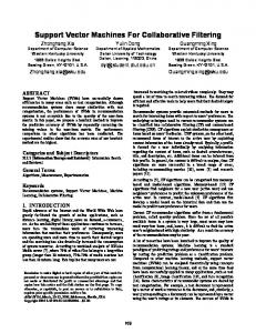
Figure 1 shows the Facebook LinkR App as it appears to users. 2 The main developer of the LinkR Facebook App is KhoiNguyen Tran, a PhD student at the Australian National University. Khoi-Nguyen wrote the user interface and database crawling code for LinkR. All of the learning and recommendation algorithms used by LinkR were written solely by the author for the purpose of this thesis.

• Text link summary from the metatags on the target link webpage. • Number of times the link has been liked. • Number of times the link has been shared. • Number of comments posted on the link. ′ • Fx,y ∈ {0, 1}: indicator of whether user x has liked item y.

Additionally, links that have been recommended by the LinkR application have the following extra features: • id ’s of users who have clicked on the link url. • Optional “Like” or “Dislike” rating of the LinkR user on the link.

4.2.3

Interaction Data

The interactions between users that we count (equally weighted) to define Int x,z are: 1. Being friends. 2. Posting an item (link, photo, video, photo, or message) on a user’s wall. Figure 1: The Facebook LinkR App showing one of the recommendations as it appears to users of the system. Users have the option of liking or disliking a recommendation as well as providing explicit feedback commentary.

3. Liking an item (link, photo, video, photo, or message) on a user’s wall. 4. Commenting on an item (link, photo, video, photo, or message) on a user’s wall. 5. Being tagged together in the same photo.

4.2 Dataset

6. Being tagged together in the same video.

Using the LinkR Facebook App developed for this project, we were able to gather data on 34,860 users and 437,023 links.

7. Two users tagging themselves as attending the same school.

4.2.1

User Data

Date that are collected and used for the user features are as follows: • Gender: male or female • Birthday: year • location id : an integer ID corresponding to the user’s specific present location (city and country) • hometown id : an integer ID corresponding to the user’s specific home town (city and country) • Fx,z ∈ {0, 1}: indicator of whether users x and z are friends. • Int x,z ∈ N: interactions on Facebook between users x and z as defined in Section ??.

4.2.2

Link Data

Data that are used for the link features are: • id of the user who posted the link. • id of the user on whose wall the link was posted. • Text description of the link from the user who posted it.

8. Two users tagging themselves as attending the same class in school. 9. Two users tagging themselves as playing sports together. 10. Two users tagging themselves as working together for the same company. 11. Two users tagging themselves as working together on the same project for the same company.

4.2.4

Live Online Recommendation Trials

For the recommendations made to the LinkR application users, we select only links posted in the most recent two weeks that the user has not liked. We use only the links from the last two weeks since an informal user study has indicated a preference for recent links. Furthermore, older links have a greater chance of being outdated and are also likely to represent broken links that are not working anymore. We have settled on recommending three links per day to the LinkR users and according to the survey done at the end of the first trial, three links per day seems to be the generally preferred number of daily recommendations. For the live trials, Facebook users who installed the LinkR application were randomly assigned one of four algorithms in each of the two trials. Users were not informed which

Algorithm Social Matchbox Matchbox SVM Nearest Neighbor

Users 26 26 28 28

Table 1: Number of Users Assigned per Algorithm. algorithm was assigned to them to remove any bias. We distinguish our recommended links into two major classes, links that were posted by the LinkR user’s friends and links that were posted by users other than the LinkR user’s friends. The LinkR users were encouraged to rate the links that were recommended to them, and even provide feedback comments on the specific links. In turn these ratings became part of the training data for the recommendation algorithms, and thus were used to improve the performance of the algorithms over time. Based on the user feedback, we filtered out nonEnglish links and links without any descriptions from the recommendations to prevent user annoyance. At the end of the first trial, we conducted a user survey with the LinkR users to find out how satisfied they were with the recommendations they were getting.

5. BASELINE COMPARISION In this chapter we discuss the first set of four SCF algorithms that was implemented for the LinkR application and then show how each algorithm performed during the live user trial, how satisfied the users were with links being recommended to them through LinkR, and the results of offline passive experiments with the algorithms.

5.1 Algorithms The CF and SCF algorithms used for the first user trial were: 1. k-Nearest Neighbor (KNN): We use the user-based approach as described in Section 2.3.1. 2. Support Vector Machines (SVM): We use the the SVM implementation described in Section ?? using the features described in Section 4.2. 3. Matchbox (Mbox): Matchbox MF + L2 U Regularization + L2 V Regularization 4. Social Matchbox (Soc. Mbox): Matchbox MF + Social Regularization + L2 Regularization Social Matchbox uses the Social Regularization method to incorporate the social information of the FB data. SVM incorporates social information in the fx,y features that it uses. Matchbox and Nearest Neighbors do not make use of any social information.

5.2 Online Results The first live user trial was run from August 25 to October 13. The algorithms were randomly distributed among the 106 users who installed the LinkR application. The distribution of the algorithms to the users are show in Table 1 Each user was recommended three links everyday and they were able to rate the links on whether they ‘Liked’ or ‘Disliked’ it. Results shown in Figure 2 are the percentage of

Like ratings and the percentage of Dislike ratings per algorithm stacked on top of each other with the Like ratings on top. As shown in Figure 2, Social Matchbox was the best performing algorithm in the first trial and in fact was the only algorithm to get receive more like ratings than dislike ratings. This would suggest that using social information does indeed provide useful information that resulted in better link recommendations from LinkR. We also look at the algorithms with the results split between friend links and non-friend links recommendations. Again, the results shown in Figure ?? are the percentage of Like ratings and the percentage of Dislike ratings per algorithm stacked on top of each other with the Like ratings on top. As shown in Figure ??, all four algorithms experienced a significant performance drop in the ratio of Likes to Dislikes when it came to recommending non-friend links. This suggests that aside from Liking or Disliking a link solely from the quality of the link being recommended, users are also more likely to Like a link simply because a friend had posted it and more likely to Dislike it because it was posted by a stranger.

5.3

Survey Results

Near the end of the first trial, the LinkR users were invited to answer a survey regarding their experiences with the recommendations they were getting. They were asked a number of questions, with the following pertaining to the quality of the recommendations: • Do you find that ANU LinkR recommends interesting links that you may not have otherwise seen? • Do you feel that ANU LinkR has adapted to your preferences since you first started using it? • How relevant are the daily recommended links? • Overall, how satisfied are you with LinkR? They gave their answers to each question as an integer rating with range [1 − 5], with a higher value being better. Results are shown in Figure 3. Their answers were grouped together according to the recommendation algorithm that was assigned to them, and the averages per algorithm are below. As shown in Figure 3, Social Matchbox achieved higher survey scores than the other recommendation algorithms, in all four questions. The results of the survey reflected the results in the online live trial and confirms that Social Matchbox was the best recommendation algorithm in the first trial.

5.4

Summary

At the end of the first trial, we have observed the following: • Social Matchbox was the best performing algorithm in the live user trial in terms of percentage of likes. • Social Matchbox received the highest user evaluation scores in the user survey at the end of the user trial. • Of the various combinations of training and testing data in the offline passive experiment, we found that

1.0

Ratio of Liked Ratings to Disliked Ratings Per Algorithm

Ratio of Liked to Disliked Recommendations From Friends

1.0

Ratio of Liked to Disliked Recommendations From Non-Friends 1.0

0.8

0.8

0.7

0.7

0.6

0.7

0.6

0.5

0.6

0.5

0.4

0.5

0.4

0.3

0.4

0.3

0.2

0.3

0.2

0.1 0.0

Ratio of Likes to Dislikes

0.9

0.8

Ratio of Likes to Dislikes

0.9

Ratio of Likes to Dislikes

0.9

0.2

0.1

Soc. Mbox

SVM Mbox Recommendation Algorithms

KNN

0.0

0.1

Soc. Mbox

SVM Mbox Recommendation Algorithms

KNN

0.0

SVM Mbox Recommendation Algorithms

Soc. Mbox

KNN

Figure 2: Results of the online live trials. The percentage of Liked ratings are stacked on top of the percentage of Disliked ratings per algorithm. Social Matchbox was found to be the best performing of the four algorithms evaluated in the first trial. *** Results of the online live trials, split between friends and non-friends. The percentage of Liked ratings are stacked on top of the percentage of Disliked ratings per algorithm. There is a significant drop in performance between recommending friend links and recommending non-friend links.

3

1

2

0

2

0

How satisfied are you with LinkR?

3

1

KNN SVM Soc. Mbox Mbox Recommendation Algorithms

5

4

3

1

KNN SVM Soc. Mbox Mbox Recommendation Algorithms

Has LinkR adapted to your preferences?

4

3

2

0

5

4

Average Rating

Average Rating

4

How relevant are the daily recommended links? 5

Average Rating

Does LinkR recommend interesting links?

Average Rating

5

2

1

KNN SVM Soc. Mbox Mbox Recommendation Algorithms

0

KNN SVM Soc. Mbox Mbox Recommendation Algorithms

Figure 3: Results of the user survey after the first trial. The survey answers from the users reflect the online results that Social Matchbox was the best recommendation algorithm in this trial. training on the UNION subset and testing on the APPUSER-ACTIVE-ALL subset best correlated with the results of the live user trial and the user survey. Training on the UNION dataset had advantages compared to training on the other data subsets, namely that it had the large amount of information of the PASSIVE data and the explicit dislikes information of the ACTIVE data. In the next chapter, we discuss new techniques for incorporating social information and show how they improve on Social Matchbox.

6. NOVEL ALGORITHMS FOR SOCIAL RECOMMENDATION 6.1 Second Trial For the second online trial, we chose four algorithms again to randomly split between the LinkR application users. Social Matchbox was included again as a baseline since it was the best performing algorithm in the first trial. The distribution count of the algorithms to the users is shown in Table 2 The four SCF algorithms are: • Social Matchbox (Soc. Mbox) : Matchbox MF + Social Regularization + L2 U Regularization + L2 V Regularization • Spectral Matchbox (Spec. Mbox): Matchbox MF

Algorithm Social Matchbox Spectral Matchbox Spectral Co-preference Social Hybrid

Users 26 25 27 25

Table 2: Number of Users Assigned per Algorithm. + Social Spectral Regularization + L2 U Regularization + L2 V Regularization • Social Hybrid (Soc. Hybrid): Hybrid + Social Regularization + L2 U Regularization + L2 V Regularization + L2 w Regularization • Spectral Co-preference (Spec. CP): Matchbox MF + Social Co-preference Spectral Regularization + L2 U Regularization + L2 V Regularization

6.1.1

Online Results

The online experiments were switched to the new algorithms on October 13, 2011. For the online results reported here, since the second live trial is still currently ongoing, we took a snapshot of the data as it was on October 22, 2011. The algorithms were randomly distributed among the 103 users who still had the LinkR application installed. The distribution of the algorithms to the users are show in Table 2 Results shown in Figure 4 are the percentage of Like ratings and the percentage of Dislike ratings per algorithm

stacked on top of each other with the Like ratings on top. First thing we note in Figure 4 is the decrease in performance for Social Matchbox, and in fact for all SCF algorithms in general. Except for Spectral Matchbox, they all received more Dislike ratings than Like ratings. What we noticed is that of the recommendations being made in the week that we switched over to the new algorithms, the majority of the links were about Steve Jobs, who had died the week previously. We believe that the redundancy and lack of variety of the links being recommended caused an increase in the Dislike ratings being given by users on the recommended links. Taking out the skewed results that follows an unusual event such as this, the relative algorithm performance was better. We again split the results again between friend link recommendations and non-friend link recommendations, with the results shown in Figure 4 being the percentage of Like ratings and the percentage of Dislike ratings per algorithm stacked on top of each other with the Like ratings on top. As shown Figure 4, all four algorithms experienced significant performance drop in the number of likes when it came to recommending non-friend links. This reflects the results of the first trial. We note the following observations from the results shown in Figures 4: • Compared to the other algorithms, Spectral Matchbox achieved the best ratio of likes to dislikes as seen, as seen in Figure 4. Combined with the results for Spectral Co-preference, Spectral social regularization in general appears to be a better way to socially regularize compared to social regularization. This comparison holds even when the results are split between friend links recommendations and non-friend links recommendations, as seen in Figure 4. • When looking at just the friend link recommendations in Figure 4, Social Hybrid was the best performing algorithm. This result comes from the user-user information diffusion among its friends that Social Hybrid learns, which could not be learned by the other SCF algorithms. Learning information diffusion thus helps when it comes to building better SCF algorithms. • Spectral Co-preference didn’t do well on friend link recommendations, however it did better on the nonfriend link recommendations. When it comes to recommending friend links, friend interaction information coming through social regularizer seems more important than implicit co-likes information provided by the co-preference regularizer. When there is no social interaction information such as with non-friend links, copreference methods with its implicit co-likes information appear much better than just vanilla collaborative filtering at projecting users into subspaces of common interest.

6.2 Summary We summarize the observations made during the second trial: • The social spectral regularization methods generally performed better in the live user trials, even when the results were split between friend link recommendations and non-friend link recommendations.

• Learning information diffusion models helps in SCF, as evidenced by the strong performance of Social Hybrid when recommending friend links. • When there is no social interaction information, learning implicit co-likes information is better than using plain CF methods. • The better performance of the social spectral regularization methods in the live trials were not reflected in the offline experiments. Perhaps there is a better metric than MAP that correlates with human preferences.

7.

CONCLUSIONS

7.1

Summary

In this paper, we evaluated existing algorithms and proposed new algorithms for social collaborative filtering via the task of link recommendation on Facebook. In Chapter 2, we outlined three main deficiencies in current social collaborative filtering (SCF) techniques and proposed new techniques in Chapters 4 and 5 to solve them; we review them here as follows: (a) Non-feature-based user similarity: We extended existing social regularization and social spectral regularization methods to incorporate user features to learn user-user similarities in the latent space. (b) Model direct user-user information diffusion: We defined a new hybrid SCF method where we combined the collaborative filtering (CF) matrix factorization (MF) objective used by Matchbox [16] with a linear content-based filtering (CBF) objective used to model direct user-user information diffusion in the social network. (c) Restricted common interests: We defined a new social co-preference regularization method that learns from pairs of user preferences over the same item to learn user similarities in specific areas — a contrast to previous methods that typically enforce global user similarity when regularizing. Having evaluated existing baselines (with minor extensions) in Chapter 4 and evaluating these new algorithms in Chapter 5 in live online user trials with over 100 Facebook App users and data for over 30,000 unique Facebook users, we summarize the main results of the paper: • Our extensions to social regularization in Chapter 4 and Chapter 5 proved to be very effective methods for SCF, and outperformed all other algorithms in the first Facebook user evaluation trial. This was reflected in the live user trial, user survey, and offline passive experimental results. However, our socially regularized SCF MF extension in Chapter 4 could still be improved by changing to a spectral approach, and this further extension in Chapter 5 generally outperformed the SCF socially regularized extension of Chapter 4. The take-home point is that a very useful form of social regularization appears to be social spectral regularization as proposed in Chapter 5.

1.0

Ratio of Liked Ratings to Disliked Ratings Per Algorithm

Ratio of Liked to Disliked Recommendations From Friends

1.0

Ratio of Liked to Disliked Recommendations From Non-Friends 1.0

0.8

0.8

0.7

0.7

0.6

0.7

0.6

0.5

0.6

0.5

0.4

0.5

0.4

0.3

0.4

0.3

0.2

0.3

0.2

0.1 0.0

Ratio of Likes to Dislikes

0.9

0.8

Ratio of Likes to Dislikes

0.9

Ratio of Likes to Dislikes

0.9

0.2

0.1

Soc. Mbox

Spec. Mbox Spec. CP Soc. Hybrid Recommendation Algorithms

0.0

0.1

Soc. Mbox

Spec. Mbox Spec. CP Soc. Hybrid Recommendation Algorithms

0.0

Soc. Mbox

Spec. Mbox Spec. CP Soc. Hybrid Recommendation Algorithms

Figure 4: Results of online live trials. The percentage of Liked ratings are stacked on top of the percentage of Disliked ratings per algorithm. Spectral Matchbox achieved the highest ratio of likes to dislikes among the four algorithms. Spectral social regularization in general appears to be a better way to socially regularize compared to social regularization. *** Results of the online live trials, split between friends and non-friends. As in the first trial, there is a significant drop in performance between recommending friend links and recommending non-friend links. • Learning direct user-user information diffusion models (i.e., how much one user likes links posted by another) can result in improved SCF algorithms in comparison to standard MF methods. To this end, our social hybrid algorithm which uses this information outperformed all other SCF methods when recommending friend links as shown in Chapter 5. • Friend interaction information coming from social regularization is more useful than the implicit co-likes information of co-preference regularization. However, when there is no social interaction information available (as in the case of recommending non-friend links), learning this implicit co-likes information outperforms plain CF methods as evidenced by the relative success of the co-preference regularization algorithm as demonstrated in Chapter 5. • Knowing what offline metrics for measuring SCF performance correlate with human preferences from live trials is crucial for efficient evaluation of SCF algorithms and also quite useful for offline algorithm tuning. In general, as most strongly evidenced in Chapter 4, it appears that evaluating mean average precision (MAP) when training on data that includes both passively inferred dislikes and explicit negative preference feedback (i.e., explicit dislikes indicated via the Facebook App), but evaluating MAP only with explicit feedback (no inferred dislikes) seems to be a train/test evaluation approach and evaluation metric that correlates with human survey feedback. Hence, this paper has made a number of substantial contributions to SCF recommendation systems and has helped advance methods for SCF system evaluation.

7.2 Future Work This work just represents the tip of the iceberg in different improvements that SCF can make over more traditional nonsocial CF methods. Here we identify a number of additional future extensions that can potentially further improve the proposed algorithms in this paper: • We used only a subset of the possible feature data in Facebook and in the links themselves. Extending the

social recommenders to handle more of the rich information that is available may result in better performance for the SCF algorithms. One critical feature that would have been useful is including a genre feature in the links (e.g., indicating whether the link represented a blog, news, video, etc.) to provide a fine-grained model of which types of links that users prefers to receive. This additional information would have likely prevented a number of observed dislikes from users regarding specific genres of links, e.g., those that do not listen to music much and hence do not care about links to music videos — even if these links are otherwise liked by friends and very popular. • Enforcing diversity in the recommended links would prevent redundant links about the same topic being recommended again and again. This is especially useful when an unusual event happens like the death of Steve Jobs and the ensuing massive amount of Steve Jobs related links that flooded Facebook. While users may like to see a few links on the topic, their interest in similar links decreases over time and diversity in recommendations could help address this saturation effect. • Another future direction this work can go to is to incorporate active learning in the algorithms. This would ensure that the SCF algorithm did not exploit the learned preferences too much and made an active effort to discover better link preferences that are available. • Probably the biggest assumption we have made in our implementations is how we inferred the implicit dislikes of users in the Facebook data. A better and method of inferring implicit dislikes will give a big boost to the SCF algorithms. As evidenced by the results of training on ACTIVE and UNION data, having a more accurate list of likes and dislikes greatly improves the performance of the SCF algorithms. • Finally, there may be a better metric than MAP for offline evaluation that more accurately correlates with live human preference and research should continue to evaluate a variety of existing SCF evaluation metrics in

order to identify what offline evaluation metrics correlate with human judgments of algorithm performance. While there are many exciting extensions of this work possible as outlined above, this paper represents a critical step forward in SCF algorithms based on top-performing MF methods and their ability to fully exploit the breadth of information available on social networks to achieve state-ofthe-art link recommendation.

8. ADDITIONAL AUTHORS Additional authors: Ehsan Abbasnejad (ANU & NICTA, email: [email protected]).

9. REFERENCES [1] Marko Balabanovi´c and Yoav Shoham. Fab: content-based, collaborative recommendation. Communications of the ACM, 40:66–72, March 1997. [2] Robert M. Bell and Yehuda Koren. Scalable collaborative filtering with jointly derived neighborhood interpolation weights. In ICDM-07, 2007. [3] Chih-Chung Chang and Chih-Jen Lin. LIBSVM: a Library for Support Vector Machines, 2001. [4] Corinna Cortes and Vladimir Vapnik. Support-vector networks. In Machine Learning, pages 273–297, 1995. [5] Peng Cui, Fei Wang, Shaowei Liu, Mingdong Ou, and Shiqiang Yang. Who should share what? item-level social influence prediction for users and posts ranking. In International ACM SIGIR Conference (SIGIR), 2011. [6] K. Lang. NewsWeeder: Learning to filter netnews. In 12th International Conference on Machine Learning ICML-95, pages 331–339, 1995. [7] Wu-Jun Li and Dit-Yan Yeung. Relation regularized matrix factorization. In IJCAI-09, 2009. [8] H. Ma, I. King, and M. R. Lyu. Learning to recommend with social trust ensemble. In SIGIR-09, 2009. [9] H. Ma, H. Yang, M. R. Lyu, and I. King. Sorec: Social recommendation using probabilistic matrix factorization. In CIKM-08, 2008. [10] Hao Ma, Dengyong Zhou, Chao Liu, Michael R. Lyu, and Irwin King. Recommender systems with social regularization. In WSDM-11, 2011. [11] A. Ng, M. Jordan, and Y. Weiss. On spectral clustering: Analysis and an algorithm. In Advances in Neural Information Processing Systems NIPS 14, 2001. [12] Kaare Brandt Petersen and Michael Syskind Pedersen. The matrix cookbook, 2008. [13] S. Rendle, L. B. Marinho, A. Nanopoulos, and L. Schmidt-Thieme. Learning optimal ranking with tensor factorization for tag recommendation. In KDD-09, 2009. [14] Paul Resnick and Hal R. Varian. Recommender systems. Communications of the ACM, 40:56–58, March 1997. [15] Ruslan Salakhutdinov and Andriy Mnih. Probabilistic matrix factorization. In Advances in Neural Information Processing Systems, volume 20, 2008.

[16] David H. Stern, Ralf Herbrich, and Thore Graepel. Matchbox: large scale online bayesian recommendations. In WWW-09, pages 111–120, 2009. [17] S. H. Yang, B. Long, A. Smola, N. Sadagopan, Z. Zheng, and H. Zha. Like like alike: Joint friendship and interest propagation in social networks. In WWW-11, 2011.