10.1109/ULTSYM.2015.0428
Newton’s Method based Self Calibration for a 3D Ultrasound Tomography System Wei Yap Tan1 , Till Steiner2 , Nicole V. Ruiter1 1 Institute
for Data Processing and Electronics, Karlsruhe Institute of Technology, Germany Email:
[email protected],
[email protected] 2 Development Ultrasonic Sensors, Pepperl+Fuchs GmbH, Germany Email:
[email protected]
Abstract—A device for 3D ultrasound computer tomography system is currently under development at KIT with the goal of high-resolution images for early breast cancer detection. With its semi-ellipsoidal positioning of 2041 ultrasound transducers around the breast in space, full 3D images can be reconstructed. Calibration process of such a complex system is very timeconsuming and difficult. This paper proposes a Newton’s method based self calibration using time-of-flight measurements between each emitter and receiver. One unique feature of this method is the separation of each potential error sources in the system and sequential calibration according to their magnitudes. This enables the analysis of each error component in the system. Simulation and application on real data have both shown sub-wavelength accuracy in the calibration results.
I.
-3 10
4
R
3 2
The current 3D USCT system can produce reflectivity, speed of sound and attenuation images of the breast. The quality of the produced images is highly sensitive to the system calibration. Some parameters of the calibration are the position of each transducer, the temperature distribution in the medium and the system response of the electronics. Besides these, sporadic errors in the transducers and human error during cabling process could also be present. With the large amount of transducers built into the system, it is a challenging task to manually calibrate the system frequently. Hence a Newton’s method based self calibration for 3D USCT is proposed. This method is designed based on the current 3D USCT system but is also applicable to arbitrary ultrasound tomography and ultrasound sensor system based on time-of-flight (TOF) measurement of the ultrasound signals. For high quality reconstruction of objects in the ROI of USCT, a TOF error less than one fourth of the wavelength (λ/4) is required.
978-1-4799-8182-3/15/$31.00 ©2015 IEEE
R E
E R
R 0
1
I NTRODUCTION
Our 3D ultrasound computer tomography (3D USCT) system aims at high-resolution images for early breast cancer detection. The current system consists of 2041 ultrasound transducers, which are positioned on a semi-ellipsoid. The positioning of the transducers was optimized for the isotropy of the 3D point spread function (PSF) in a defined semiellipsoidal region of interest (ROI) with semi-axes of 5 cm and 10 cm [1].
R E
R
R
1 0
R E
R
2
3
4 10-3
TAS
Fig. 1. The top figure shows schematic diagrams of single transducer array with its 4 emitters and 9 receivers (left) and a color-coded photo of a manufactured transducer array in a TAS. The TAS and the USCT aperture with its 157 TASs is shown in the lower figure.
II.
BACKGROUND
A. USCT Geometry The current 3D USCT system at KIT has a semi-ellipsoidal arrangement of 628 emitters and 1413 receivers. The elements are grouped into 157 transducer arrays (TAS) with 4 emitters and 9 receivers each as shown in Fig. 1. These transducers have a center frequency of 2.5 MHz with 50% bandwidth, as well as an opening angle of approximately 30◦ to its surface (at 6 dB). The semi-ellipsoidal aperture has a diameter of 26 cm and a depth of 18 cm. Rotational and translational movements of the aperture are applied to create additional virtual positions of the ultrasound transducers. B. Error Sources The error sources leading to TOF errors in the USCT can be categorized into mechanical and electrical errors. Additionally, the medium of propagation for the ultrasound waves, which is water in the case of USCT, can influence the accuracy of TOF detection. The mechanical errors are mainly caused by the deviation of the manufactured USCT geometry from the original design.
2015 IEEE International Ultrasonics Symposium Proceedings
When constructing the USCT, the tolerance of the machining introduced deviation in the geometry. Besides that, small deviation of the center of the transducer array to the center of the TAS is expected during the mounting process of the transducer array in each TAS. After exchange of malfunctioning TAS and mounting of a new TAS, the position of the TAS is expected to be slightly different. A calibration of the USCT geometry is thus necessary. Finally, it is also expected that the USCT aperture undergoes thermal expansion and shrinkage as the temperature of the system changes. Electrical errors are caused by characteristics of electronics in the USCT system. One example is the delay between the transmitting and receiving of ultrasound wave and the excitation of the piezo-element. Similarly, transient characteristics of analogue to digital conversion and vice versa also introduce delays to the system. These delays causes errors in the TOF determination and hence the focusing of the imaging. Other electrical errors are malfunctioning amplifiers and transmitter electronics in the TAS. For example, when a transmitter is not transmitting any ultrasound signal, no TOF information would be available from this element. Any sporadic malfunctioning of other electronics in the system could also affect the accuracy of TOF determination, and should be detected and compensated. As TOF detection is strongly coupled to the assumed speed of sound [4], the accuracy of temperature measurement in the medium is important. In USCT, each TAS is equipped with a temperature sensor mounted behind the matching layer of the transducer array. Due to the transition through the matching layer, an offset in the measured temperature is expected. In order to compensate this, the USCT is also equipped with two PT100 temperature sensors from JUMO GmbH & Co. KG. Table I summarizes the error sources and gives their magnitudes. TABLE I.
E RROR SOURCES AND THEIR MAGNITUDE IN USCT
Error source Machining accuracy Center deviation in each TAS Radial offset of each TAS Rotation of each TAS Aperture material coefficient of thermal expansion (POM-C) Electrical mechanical delay Temperature offset in TAS Temperature error in TAS Potential jitter of electronics
III.
Error magnitude ≤ 10 µm x, y ≤ 1 mm, z ≤ 300 µm ≤ 10 µm ≤ 2◦ 1.1·10−4 K−1 = ˆ 28.6 µm K−1 ≈ 1 µs = ˆ 1.5 mm ≈ 3 ◦C = ˆ 1.5 mm ≈ 1 ◦C = ˆ 0.5 mm 20 MHz = ˆ 76 µm
at at at at
25 ◦ C 25 ◦ C 25 ◦ C 25 ◦ C
M ETHODS
A. Strategy This work proposes a self calibration method for arbitrary ultrasound transducer systems including 3D USCT based on TOF measurements. It is assumed that the position of each transducer is known to a certain accuracy, and the medium is not necessarily homogeneous. This means that the speed of sound (SOS) changes along the propagation path are possible. Lastly, an overall system delay consisting of a delay due to transient response of the transducers and the characteristics of the electronics, and a TOF deviation due to thermal expansion of the USCT aperture is expected. The calibration problem can
be summarized into the following TOF equation: ||si − rj || = cij · (tij − τsi − τrj )
(1)
with vectors si and rj as positions of emitter i and receiver j in a 3D coordinate system. The TOF of the shortest direct path between the two transducers is given by tij with the mean speed of sound along the path as cij calculated from the given temperature distribution in medium. The transmission and reception delays are modelled with τsi and τrj . These delays are specific for a transducer element throughout the system. The goal of the calibration process is to find a unique solution of all unknowns by solving a large nonlinear equation system of Eq. (1). This work proposes the use of Newton’s method to solve the equation system iteratively. This work separates the calibration problem into individual steps according to their error magnitude: positions, temperature and delay calibration. Besides that, pre-filtering of each TOF determined is necessary to exclude malfunctioning emitter and receiver combinations from the equation system. As the opening angle of the main lobe of an ultrasound transducer is limited, there is only a limited number of emitter and receiver combinations, which provide useful TOF measurements. For the USCT geometry, we have a total of 157×4×157×9 = 887364 emitter and receiver combinations. Due to the limitation of directivity, this total is reduced to about 14% at 128268 combinations. B. Newton’s Method One well-known method for solving a nonlinear equation system is the Newton’s method. The Newton’s method [2] searches iteratively for a better approximation to the solution which satisfies: x : f (x) = 0 with x as the unknowns and f (x) a differentiable function. Starting with a good approximation of the solution, vector x can be updated by the following equation: xn+1 = xn − J −1 (xn ) · f (xn ) (2) where J(xn ) is the Jacobian matrix, which contains the firstorder partial derivatives of f (xn ). The iterations are continued until a predefined accuracy is achieved. C. Pre-Filtering In the USCT system at KIT, TOF detection is performed by applying a matched filter onto the received signal and detecting the maximum of the correlation result. The received signal is called A-scan and is sampled at 10 MHz. This signal processing method is generally robust against high noise levels in the signals [3]. However, malfunctioning of the transducer elements can still affect the TOF detection. For instance, a malfunctioning emitter, which does not transmit any ultrasound signal, will result in false-positive TOF detection by the matched filter. Other distortions in the signal, such as high frequency spikes, can also affect the accuracy of TOF detection. Hence, it is necessary to pre-filter the TOFs before using them for the calibration process. 1) SNR filtering: One possibility for finding malfunctioning emitter and receiver is to measure the signal-to-noise ratio (SNR) of each A-scan. Emitter and receiver combinations with SNR much lower than the average will be blacklisted. Transducer elements with frequency higher than a pre-defined
threshold in the blacklist will be excluded from further calibration process. 2) TOF detection error filtering: Since A-scans with artefacts, such as high frequency spikes, tend to have large maximum amplitudes, this might not be detected by the SNR filtering. A possible strategy is to analyse the standard deviation of the delay assigned to each transducer element after the calibration. If the detected delay has large deviations from the overall system delay, the emitter and receiver combination of the corresponding A-scan will be blacklisted. Emitters and receivers with frequent occurrence in the blacklist will be excluded from the following calibration process. D. Position Calibration When performing the position calibration, it is assumed that the magnitude of system delays (τsi , τrj ) is negligible and the SOS in medium is accurate. Eq. (1) can be simplified as: (3)
We summarized the coordinates of each emitter si = (xsi , ysi , zsi ) and receiver rj = (xrj , yrj , zrj ) of an ultrasound transducer system with m emitters and n receivers into a single vector x = [s1 , ..., sm , r1 , ..., rn ]T and rewrite Eq. (3) as: f (si , rj ) = ||si − rj || − cij · tij = 0.
E. Temperature Calibration The deviation of the measured temperature from the actual temperature in the medium along the signal path influences the SOS used in determining the distance travelled by the ultrasound signal from emitter to receiver. The temperature calibration assumes that the transducer coordinates and TOF measured have much lower error magnitude than the estimated SOS, which is a function of the medium temperature. With this assumption, Eq. (1) can be re-formulated as: (5)
(7) (8) (9)
Eq. (8) and (9) limit the delays to positive values. G. Calibration Process Sorting the error magnitudes listed in table I, we designed the sequential calibration process as shown in Fig. 2 for the USCT system, which starts with error sources with the largest magnitude and uses the calibration of the previous step. The goal of the calibration process is to minimize the residuum of the equation system in each step. TOF Detection
SNR Filtering
TOF Detection Error Filtering
Delay Calibration
Temperature Calibration
Position Calibration
Fig. 2. Suggested calibration process of our USCT system arranged according to error magnitudes
(4)
The equation system to be solved is Eq. (4) for all possible emitter and receiver combinations. Starting with an initial guess of vector x, the equation system is solved using the Newton’s method.
f (Tsi , Trj ) = ||si − rj || − c¯(Tsi , Trj ) · tij = 0,
f (τsi , τrj ) = ||si − rj || − cij · (tij − τsi − τmj ) = 0 f (τsi ) = |τsi | − τsi = 0 f (τrj ) = |τrj | − τrj = 0.
IV.
R ESULTS
A. Simulated Arbitrary Ultrasound Sensor System & USCT We evaluated the self calibration method with a simulated ultrasound sensor system consisting of 75 emitters and 75 receivers, which are positioned randomly on a sphere with radius of 12 cm. All transducer elements points towards the center of the sphere. Simulated Ultrasound Sensor System Emitter Receiver
-0.1 -0.05
z
||si − rj || = cij · tij .
it is also assumed that the error magnitudes in position and temperature data are negligible. We introduce the vector τ = [τs1 , ..., τsm , τr1 , ..., τrn ]T and the equations:
0 0.05 0.1
where the temperatures at emitter i and receiver j are summarized in vector x = [Ts1 , ..., Tsm , Tr1 , ..., Trn ]T . Additionally, an extra equation can also be included to correct an overall system offset to any calibrated temperature sensor: ¯ − Tcali = 0. f (x) = x
0.1 0.05 0 -0.05 -0.1 y
0.1 0 -0.1
x
(6)
F. Delay Calibration For the delay calibration, each emitter and receiver is assigned with a delay τsi and τrj as given in Eq. (1). The main goal of the delay calibration is to determine an overall system delay, τ¯ = mean(τ ), which best describes the overall transient characteristic of the piezo-elements and the electronics. The delay correction is not done individually for each transducer element due to the risk of over-correcting the TOF-deviation caused by difference of transducer positions to their assumed coordinates. During the delay calibration,
Fig. 3. Simulated ultrasound sensor system. The axes in the diagram are given in meter.
The simulation was conducted with a sample rate of 100 MHz. Potential jitter due to system frequency was set at 20 MHz and the A-scans were sampled at 10 MHz. For the TOF detection, the A-scans were re-sampled at 100 MHz for higher TOF resolution. The simulation was performed on the simulated ground truth with added errors. Table II shows the simulated error magnitudes and the calibration error as average of the differences to the ground truth. Results in Table II demonstrate the ability of the self-calibration strategy
in detecting and correcting each error source. At the end of the calibration process, only a position error of around 16 µm and a residuum or an uncertainty of 3 µm remained, which is very small compared to the wavelength λ = 0.6 mm of the ultrasound center frequency used. The position error was limited by the sample rate used during the simulation. Similarly, a simulation was done with the USCT geometry and calibrated. Due to the limited angular characteristic of the transducer elements, only the first 114 TASs in the first five layer of the USCT aperture were selected for the calibration process. The result is also presented in Table II. TABLE II.
no ground truth for the real system, the electrical delay and temperature offset listed in Table III were the detected values The residuum of the position calibration is given as position uncertainty. TABLE III.
Error Sources Electrical delay Temperature offset Temperature error Position uncertainty (mean) Position uncertainty (SD)
C ALIBRATION ERROR OF SIMULATIONS
Error Sources Simulated Error Simulated sensor system Electrical delay 1.2 µs Temperature offset -3 ◦ C Temperature error 1 ◦C Position error ≤ 1 mm Simulated USCT system Electrical delay 1.2 µs Temperature offset -3 ◦ C Temperature error 1 ◦C Position error ≤ 1 mm
Calibration Error 0.025 µs -0.554 ◦ C 0.021 ◦ C mean = 16.29 µm, SD = 4.08 µm 0.175 µs -0.517 ◦ C 0.031 ◦ C mean = 17.79 µm, SD = 3.62 µm
Since the USCT geometry has a more restricted distribution of transducers i.e. only on a semi-ellipsoid as compared to a full sphere, the increase in calibration error was expected. In both cases, the Newton’s method converges within 15 iterations to a precision of 0.1 µm. Fig. 4 shows the full width at half maximum (FWHM) analysis of a simulated point scatterer reconstructed with and without calibration. It is shown that without delay calibration, the reconstructed point scatterer was unfocused. Once the delay is calibrated, the FWHM was improved to λ/2. A small additional improvement was achieved when the position calibration was conducted, as it has the lowest error magnitude.
C ALIBRATION RESULT BASED ON REAL USCT DATA Calibration Result Mean Standard Deviation 1.2152 µs 0.0126 µs -2.5955 ◦ C 0.0765 ◦ C 0.0662 ◦ C 0.0178 ◦ C 141.53 µm 0.820 µm 285.84 µm 63.58 µm
We noticed that the position uncertainty of 141.53 µm, approx. λ/4, was much larger in the simulated experiments. In the absence of ground truth, this value represents the summed uncertainty in all error sources after the calibration in the TOF detection. V.
D ISCUSSION
The proposed Newton’s method based self calibration for arbitrary ultrasound sensor system based on USCT shows ability to quantify and compensate for multiple error sources as shown in the simulations. Application on real data achieves a λ/4 position and TOF uncertainty, which satisfied the requirement for high quality USCT images. The are 10362 unknowns to be calibrated for the current USCT system. The Jacobian matrix for simultaneously calibrating them with all emitter and receiver combinations requires at least 10 GB at double precision, hence limiting its implementation on normal PCs.
Additionally, these unknowns are the complement of each other, for example the temperature calibration and the scaling of the USCT geometry with position calibration. Simultaneously calibrating them in a single equation system leads to Analysis of Full Width at Half Maximum (FWHM) multiple local minima. Based on these observation, we opted Analysis of Full Width at Half Maximum (FWHM) the presented sequential calibration strategy. The calibration #10 -4 Calibrated Geometry 8 Original Geometry Calibrated Geometrystrategy also provided an analysis method for each error Original Geometry - with Delay -with Delay 7.5 component in the system. The calibration process described in Max of Calibrated Geometry Max of Calibrated Geometry Max of Original Geometry Max of Original Geometry Fig. 2 can be adapted to other sensor systems with descending Max of -with Delay Max of -with Delay 7 2.777e-04 m 2.777e-04 order of the magnitudes of the error sources. The absence of 3.006e-04 m 3.006e-04 6.5 the ground truth for real data currently limits the possibility to pinpoint the reason for the larger residuum when applied 6 on real USCT data compared to the simulations. Further investigation on reducing the residuum will be conducted. It 5.5 is believed that other unknown error sources can be found and 5 compensated. Besides that, the proposed method will also be tested for air-borne ultrasound sensor system. 4.5 5
0.5
5
0.5
0.
25
0.
0. 0.5 5
25
0.
5
0.
0.5
2 0.
25
25
0.
5
0.2
0.
25
0.2
0.5
0. 25
0.25
0.25
x
5
5
35
4 6 y
0.
5
0.5
0.2
5 0.2
4
0.5
00.5 .5
0.2
5
5
0.2
0.25
0. 25
25
4
0.2 05 .25
0.25
5
0. 5
5
5
0.2
0.2
0.2 05 .25
0.
0.25
0.2
5
0.25
0.2
0.2
0.5
00.5 .5
5 7
6 y
8
7 #10 -4
R EFERENCES
8 #10 -4
Fig. 4. Full width at half maximum (FWHM) analysis of a simulated point scatterer in the USCT system. The axes are given in meter.
B. Application on Real Data The applied USCT measurement data was taken with ten aperture positions at a water temperature of 25 ◦ C. Data from each aperture position was used separately, in order to investigate the stability of the algorithm. Since there is
[1]
G.F. Schwarzenberg, Untersuchung der Abbildungseigenschaften eines 3D-Ultraschall-Computertomographen zur Berechnung der 3DAbbildungsfunktion und Herleitung einer optimierten Sensorgeometrie Dissertation, Karlsruher Institut fuer Technologie, 2008. [2] R.P. Brent, Some Efficient Algorithms for Solving Systems of Nonlinear Equations SIAM Journal on Numerical Analysis, Vol. 10, No. 2, pp. 327-344, 1973. [3] Steven W. Smith, Digital Signal Processing: A Practical Guide for Engineers and Scientists Newnes, 2013. [4] W. Marczak, Water as a standard in the measurements of speed of sound in liquids J. Acoust. Soc. Am. 102(5), pp 2776-2779, 1997.