economics decision model (Heady and Dillon, 1961; Dillon and Anderson, 1990). Lowenberg-DeBoer and Boehlje (1996) show that the traditional uniform rate.
Back to the Table of Contents
Previous Manuscript
Next Manuscript
NITROGEN MANAGEMENT IN CORN USING SITE-SPECIFIC CROP RESPONSE ESTIMATES FROM A SPATIAL REGRESSION MODEL Rodolfo Bongiovanni National Institute for Agricultural Technology (INTA) Manfredi, Córdoba Argentina James Lowenberg-DeBoer Department of Agricultural Economics Purdue University West Lafayette, Indiana
ABSTRACT Adapting variable rate technology (VRT) to Argentine conditions requires methods that use inexpensive information and that focus on the inputs and variability common to Argentine maize and soybean growing areas. The goal of this study is to determine if spatial regression analysis of yield monitor data can be used to estimate the site-specific crop Nitrogen (N) response needed to fine tune variable rate fertilizer strategies. N has been chosen as the focus of this study because it is the most commonly used fertilizer by corn farmers in Argentina. The methodology uses yield monitor data from on-farm trials to estimate site-specific crop response functions. The design involves a strip trial with a uniform N rate along the strip and a randomized complete block design, with regression estimation of N response curves by landscape position. Spatial autocorrelation and spatial heterogeneity are taken into account using a spatial error model and a groupwise heteroskedasticity model. A partial budget is used to calculate uniform rate and VRT returns. First year data indicate that N response differs significantly by landscape position, and that VRA for N may be modestly profitable on some locations depending on the VRT fee level, compared to a uniform rate of urea of 80kg ha-1. A more complete analysis will pool data over many farms and several years to determine if reliable differences exist in N response by landscape position or other type of management zone. The study is planned for four years. The purpose of this preliminary analysis is to show how spatial regression analysis of yield data could be used to fine tune input use. Keywords: Precision agriculture, variable rate nitrogen, profitability, spatial autocorrelation, Argentina. Copyright © 2000 ASA-CSSA-SSSA, 677 South Segoe Road, Madison, WI 53711, USA. Proceedings of the Fifth International Conference on Precision Agriculture.
INTRODUCTION Technologies based on computerized information and global positioning systems (GPS) are transforming large-scale commercial agriculture throughout the world. This technology is often labeled “precision agriculture” and is giving new life to the old idea of site-specific management by reducing the cost of crop information and variable rate input application. The underlying concepts of site-specific management are transferable from place to place, but fine-tuning production systems are necessarily site-specific because soils, climate and economic conditions vary. Argentine producers and agribusiness companies face some special problems in adapting precision agriculture to their conditions. While yield monitoring in Argentina has followed a similar adoption path to that of North America, variable rate application of inputs has not been widely used because of the high cost of soil sampling and relatively low fertilizer use. Furthermore, management induced variability in Argentina is less than in the US or Canada (Lowenberg-DeBoer, 1999). Commercial laboratory analysis of soil samples in Argentina ranges from $40 to $70 per sample, compared to the $3 to $8 charge for the basic analysis in the US. The cost of soil sampling makes the intensive grid or soil type sampling used in North America prohibitively expensive. The maize and soybean areas of North America have been farmed for a century or more. Before motorized mechanization, they were divided into small five to ten hectare fields. Old fence rows, windbreaks, feedlots, and other artifacts of past management create complex spatial patterns. Spreading errors and other mismanagement of fertilizer have added to this spatial complexity. In Argentina, widespread maize and soybean production is more recent than in the US and Canada. Since fertilizer use has been modest, fertilizer mismanagement has not created substantial spatial patterns. Also, the size of the fields has usually been quite large, reducing the effect of old field boundaries and other artifacts of past management. Adapting variable rate technology (VRT) to Argentine conditions will require methods that use inexpensive information, and that focus on the inputs and variability common to Argentine maize and soybean growing areas. The objectives of this study are to: 1) determine if spatial regression analysis of yield monitor data can be used to estimate the site-specific crop N response needed to fine tune variable rate fertilizer strategies, 2) estimate the profits for site-specific N management using the crop responses estimated under objective (1), and 3) compare profits from site-specific N management using crop response functions with uniform rate management and proposed spatial management strategies. N has been chosen as the focus of this study because it is the most commonly used fertilizer by corn farmers in Argentina. The methodology utilizes
yield monitor data from on-farm trials in southern Córdoba Province to estimate site-specific crop response functions with low cost independent variables such as landscape position, topography and soil color. Producers and crop consultants can use the site-specific crop response methodology to guide N application and increase profits. The hypotheses are: 1) There is spatial autocorrelation and heteroskedasticity in corn yield response to N rates across landscape positions. 2) Maize N response varies by landscape position, 3) VRT N application would be profitable on average if VRT fees are under $6 ha-1. Expected Results: The principle expected result will be information leading to improved N management throughout the maize and soybean growing areas of Argentina, especially those in Córdoba Province. From a methodological point of view, the results will show the consequences of ignoring spatial autocorrelation in a regression model when it is in fact present. Potential Users: The potential users are producers, crop consultants, and fertilizer dealers throughout the corn and soybean-growing areas of Argentina. Researchers in the area of precision agriculture will be pointed to the importance of spatial dependence in regression analysis models. LITERATURE REVIEW Site-specific fertilizer application is an old idea. In the US, the first extension recommendations on intensive soil sampling and variable rate fertilizer application appeared in 1929 (Linsley and Bauer, 1929). The recent resurgence of interest in the idea can be linked to the availablity of GPS and information technology (IT) which lower information and VRT implementation costs dramatically. VRT fertilizer was the earliest commercially available precision agriculture service in the US. Currently, about 50% of the approximately 7500 retail fertilizer dealers in the US offer the service in the US (Akridge and Whipker, 1999). In contrast, only ten VRT fertilizer applicators were being used in Argentina in 1998 (Bragachini, 1999). In the US, VRT fertilizer is a common practice among producers of higher value field crops, such as sugar beets. Many US maize and soybean farmers have tried VRT fertilizer, but doubts remain about its profitability (Lowenberg-DeBoer and Swinton, 1997). Swinton and Lowenberg-DeBoer (1998) review studies of the profitability of site-specific N, phosphorus (P) and potassium (K) fertilizer application based on intensive soil sampling, using either grids or soil type. They conclude that VRT fertilizer is often profitable for higher value field crops but seldom profitable for extensive dryland crops like wheat and barley. For maize and soybeans, VRT fertilizer often fails to cover the added costs of soil sampling and VRT application. Key methodological problems identified in these studies include: failure to charge soil sampling, analysis and VRT application fees, and use of
simulation models which assumed target yields would be achieved. LowenbergDeBoer and Aghib (1999) use on-farm trial data from the eastern Corn Belt to show that VRT P & K just about covers costs as a stand-alone practice, and that it may have potential to reduce risks. Bongiovanni and Lowenberg-DeBoer (1998) show that VRT lime is modestly profitable in the Eastern Cornbelt. On-farm trials on the Sauder farm in central Illinois showed a 941 kg ha-1 yield increase for corn grown in an integrated site-specific management system which combined VRT NPK, lime, and plant population (Finck, 1998). Many alternatives to intensive soil sampling have been proposed for N management, but no method has been widely accepted as better than uniform rate application. Pan et al. (1997) review studies of spatial variability of N in annual field crops. They note that current university and industry N recommendations in North America may not be very useful for site-specific management because they are broad compromises intended to be used regionally. Pan et al. also indicate that N available to the plant at any one location and time depends on many factors, including organic matter in the soil, previous crop, manure applications, recent temperature and rainfall patterns, and leaching losses. Because N is spatially and temporally dynamic, N soil tests, stalk nitrate tests, and leaf nitrate tests are not necessarily a good basis for making N fertilizer decisions, even when these tests are available and affordable. The proceedings of the international conferences on precision agriculture held in Minnesota contain a wide variety of N management proposals (Robert et al., 1992, 1994, 1996, 1998). The 1996 and 1998 proceedings contain 52 papers focusing on N management. In addition to intensive soil sampling, proposed sources of spatial information to guide N application include: aerial photography and satellite remote sensing, landscape position, topography, yield and grain protein maps, soil type, and chlorophyll sensors. Making better N management choices is not simply a case of understanding N dynamics, but also requires a decision support system that effectively uses relatively low cost data to predict yields and profits under alternatives. Many simulation and statistical models have been proposed (see various papers in Robert et al., 1994, 1996, 1998). The simulation process models have been calibrated to mimic spatial variability in specific fields, but it is not clear that this can be generalized. Most crop growth models currently lack many of the factors that drive spatial variability (e.g. topography, microclimate, water flow). Crop growth models are great research tools, but it is unlikely that producers and crop consultants will be willing to invest the time and resources to calibrate and validate the models for specific fields. Categorical models ranging from simple analysis of variance to clustering and fuzzy set analysis can be used to identify management areas, but leave the question of optimal N application unanswered. Several researchers have used ordinary least squares (OLS) regression to help estimate crop responses, but with mixed results (see for instance, Khakural et al., 1998; Coelho et al, 1998, Mallarino et al., 1996). Regression crop response functions have the advantage of fitting easily into the traditional crop production
economics decision model (Heady and Dillon, 1961; Dillon and Anderson, 1990). Lowenberg-DeBoer and Boehlje (1996) show that the traditional uniform rate production economics decision framework can easily be modified for site-specific management. Software that combines regression and optimization could easily be developed using well-known algorithms. Annual updating of response coefficients to reflect genetic improvement and other management changes could be automated. These updates would reestimate the response with yield monitor data. Kessler and Lowenberg-DeBoer (1998) show that spatial correlation of regression error is important in yield monitor data. Because of this spatial correlation, OLS regression gives biased coefficient estimates. Anselin (1988) outlines spatial regression models that adapt generalized least squares regression to spatial data. These spatial regression models have been used mainly for regional economics analysis. The authors do not know of any attempt to estimate spatial regression models with yield monitor data. Spatial Econometrics Anselin (1999a) defines spatial econometrics as a subfield of econometrics that deals with the treatment of spatial interaction (spatial autocorrelation) and spatial structure (spatial heterogeneity) in regression models for cross-sectional and panel data. Spatial econometrics is distinct from spatial statistics in the same ways that econometrics is distinct from statistics in general. These differences stem from the type of data being analyzed and the ways in which the results are used. A difference between geostatistics and spatial econometrics is the way in which the results are used. A primary concern of many studies in the geographical literature is with identifying and estimating spatial structure of a data set (Anselin, 1988). In short, geostatistics focuses on producing a better map. Spatial econometrics is concerned with estimating the relationships between variables that have spatial structure. Those estimated relationships are then used to calculate outcomes of economic interest (e.g. yields, profits, costs), which are in turn the basis for management decisions. When the data has spatial structure, spatial econometrics can produce more accurate estimates than conventional econometrics. Spatial Autocorrelation Spatial autocorrelation, or more generally, spatial dependence, is the situation where the dependent variable or error term at each location is correlated with observations on the dependent variable or values for the error term at other locations. The general case is formally: E[yi yj] ≠ 0, or E[ i j] ≠ 0 for neighboring locations i and j, where i and j refer to individual observations (locations) and yi(j) is the value of a random variable of interest at that location. This specification is too general to allow for the estimation of potential N times (N-1) interactions from N observations. Therefore, the form of the spatial dependence is given structure
by means of a spatial weights matrix (W), which reduces the number of unknown parameters to one, i.e,. the coefficient of spatial association in a spatial autoregressive or spatial moving average process (Anselin, 1992). Spatial autocorrelation in yield data is present as the coincidence of value similarity with location similarity; i.e., high or low values for a random variable tend to be surrounded by neighbors with similar values. Since the values of yield factors at some point in the field depend on the values of other points in the field, the data from this field will present spatial autocorrelation. The presence of positive autocorrelation implies that a sample contains less information than an uncorrelated one. To carry out accurate statistical inference, this loss of information must be explicitly be taken into account in estimation and diagnosis tests. Therefore, classical statistical tests on spatial series must be combined with tests of spatial autocorrelation to assess the validity of drawing inferences (Anselin and Bera, 1998). Spatial Regression Models Anselin (1999a) outlines two important alternative models to deal with autocorrelation: the spatial lag model and the spatial error model. Since the estimates from the spatial regression model are going to be used in a decision model to measure costs, profits, etc., then accurate estimates are needed. This is the main role of an error model, whereas, in the lag model, the main role is to predict the spatial pattern. The preliminary analyses of the corn yield data point to autocorrelation in the variables that are not in the model. Obviously, there are other variables that influence yield, and these are very autocorrelated. This problem is solved, correcting for spatial autocorrelation, through the use of one of the two error models. In the spatial lag model, the spatial autocorrelation pertains to the dependent variable, y. This alternative is formalized in a mixed regressive, spatial autoregressive model: y = Wy+X + , where y is the vector of yield points, is the spatial autoregressive coefficient, Wy is a spatially lagged dependent variable, X is a matrix with observations on the explanatory variables, and and ~ (0, σ2) are, respectively, the estimated coefficients and the normally distributed random error terms. The null hypothesis of no autocorrelation corresponds to: H0: =0. If spatial autocorrelation of y exists and is ignored, the OLS estimates will be biased and all inference based on the standard regression model (i.e., the model without the Wy term) will be incorrect. In a sense, this is similar to the consequences of omitting a significant explanatory variable in the regression model. The spatial error model, or spatial dependence, is expressed by means of a spatial process for the error terms, either of an autoregressive or a moving average form. Such an autoregressive process can be expressed as: y = X + . In the spatial error model, = W + , where is the autoregressive coefficient for the spatial error term W . The error term is assumed to be normally distributed as
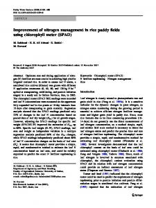
N(0,σ2I). The null hypothesis is of the form: H0: =0 or, the error term is uncorrelated. It turns out that the tests for the presence of either form of spatial error dependence are the same. The consequences of ignoring spatial error dependence are that the OLS estimator remains unbiased, but is no longer efficient since it ignores the correlation between error terms. As a result, inference based on t and F statistics will be misleading, and indications of fit based on R2 will be incorrect. Spatial autocorrelation inflates R2, deflates standard errors for slope parameters, and overestimates the t values for inferential tests (Anselin, 1992). Weights Matrix One of the major distinguishing characteristics of spatial regression models is that the spatial arrangement of the observations is taken into account. This is formally expressed in a spatial weights matrix, W, with elements wij, where the ij index corresponds to each observation pair. The nonzero elements of the weights matrix reflect the potential spatial interaction between two observations. This may be expressed, for instance, as simple contiguity (having a common border), distance contiguity (having centroids within a critical distance band), or in function of the inverse distance. Elements that are zero indicate a lack of spatial interaction between two observations (by convention, the diagonal elements of the weights matrix are set to zero) (Anselin, 1992). DATA N response data was collected from strip trials on four farms in the Río Cuarto area, Córdoba Province, Argentina, in the 1998-99 crop season. The complete, forthcoming study is projected for four crop seasons. Site-specific N response functions will be estimated for each farm using Anselin’s spatial regression procedures. The site-specific N responses will be used to estimate the N application by landscape position that maximizes expected profits. Profits will be estimated for uniform application and for VRT N by landscape position. The experimental design for the trials is a randomized complete block strip trial that includes at least three different types of soils in terms of landscape (hilltop, slope, and low). The strips are wider or equal to the corn header width, with a zero N control and four/five other rates of elemental N: 29, 53, 66, 106 and 131.5 kg ha-1 of elemental N for the “Las Rosas” farm (Fig. 1); 29, 52, 77, 102 and 129 kg ha -1 for the “La Morocha” farm; 24, 59, 78 and 105 kg ha-1 for the “El Piquete” farm; and finally: 26, 47, 75, 101 and 122 kg ha-1 for the “Justiniano Posse” farm. The N rate is constant for the whole strip. Since the regression estimation procedure is flexible, N rates need not be the same from farm to farm. The highest N rate for each field is higher than the expected yield maximizing level. Each field has at least three blocks. Within each block, treatments are randomized. The
treatments are the same and on the same location each time maize is grown in that field. The N source is either urea-ammonium nitrate solution (UAN), or urea. Data was collected with a standard Ag Leader yield monitor. Yield files include data-point information about yields, latitude, longitude, elevation, and moisture. Since the raw data includes data yield points that are closer within the same row than between rows, these data yield points were averaged for a withinrow distance equivalent to the between-rows distance, such that a distance weights matrix could be calculated. Future analysis will be done in a GIS software capable
N rates in kg ha-1 of elemental N: 29
53
0
106
66 132 29
53
0
106 66 132 29
53
0
106 66 132
Topography 1 (LowE) Topography 2 (Slope E) Topography 3 (Hilltop)
Topography 4 (Slope W) Topography 5 (Low W)
Figure 1. Experimental design diagram for the “Las Rosas farm”
of creating grids over the observations, so that annual data will be compared in different layers. METHODOLOGY Response function estimation using spatial econometric techniques requires three steps: 1) Specification tests and diagnostics for the presence of spatial effects, 2) The formal specification of spatial effects in econometric models, and 3) The estimation of models that incorporate spatial effects. Response estimates are made for the first year to obtain preliminary results, to show how yield data should be handled for economic analysis, and to elicit feedback from producers and crop consultants. After the fourth year’s data is collected, the data will be pooled by farm and a single response function will be estimated. A quadratic response function will be tried first in all cases; alternative functional forms will be tested. The data will be analyzed using two software packages: ArcView and SpaceStat (Anselin, 1999b). The first hypothesis was tested by running a classical OLS regression in SpaceStat with diagnostics tests. The corn response to N was estimated as quadratic for both the full pass data set and by landscape position:
Yield =
0
+
1
Ni +
2
N i2 + , where: Yield = corn yield (from a yield monitor
with GPS) and Ni = N rate. Five different topography areas were evaluated through dummy variables as Spatial Regimes in SpaceStat. The dummy variable constraint was that the sum of dummy variable coefficients is equal to zero. Thus the coefficients are the difference between the intercept or slope for a given landscape position and the average slope or intercept. A t test (z test in the spatial regression model) determined if the landscape and the slope interaction terms are statistically significant. It should be noted that the conventional 1% and 5% significance levels are useful benchmarks, but not magic. In the corn yield model under study, contiguity between spatial units is defined as a function of the distance that separates them. The relevant neighborhood is defined as all grid center points within 13 meters. The 13 meters are measured from the center point of the grid. All points in the neighborhood are of equal weight in the spatial weight matrix. For the estimation of spatial regression models, the spatial weights matrix is row-standardized to yield a meaningful interpretation of the results. The row standardization consists of dividing each element in a row by the corresponding row sum. Each element in the new matrix thus becomes: wij / j w ij. The resulting distance matrix provides more information about the observations, enabling the weights to capture the proximity of about eight neighbors on average, which is equivalent to adopting a “Queen” criterion (having a border or a corner in common) (Anselin, 1988). SpaceStat (Anselin, 1999b) contains three diagnostics tests for spatial dependence in the error model: The first test is Moran’s I, to measure spatial autocorrelation in regression residuals. It is formally similar to a Durbin-Watson statistic. The second test listed in the SpaceStat regression output is the Lagrange Multiplier (LM). The LM test is a test on the slope or gradient of the LogLikelihood function. It is an asymptotic test, which follows a χ_ distribution with one degree of freedom. The third test is the Kelejian-Robinson statistic. This test is obtained from an auxiliary regression of cross products of residuals and cross products of the explanatory variables The statistic is a large sample test and follows a χ_ distribution with P degrees of freedom, where P is the number of explanatory variables. These tests not only will serve as a diagnostics of autocorrelation and heteroskedasticity, but also will indicate which spatial regression model should be used: error or lag model. On the other hand, three diagnostics tests of heteroskedasticity are implemented in SpaceStat, but only two are reported at any time. The first reported test is either the Breusch-Pagan (BP) test, or its studentized version, the Koenker-Bassett (KB) test. Which of the two is reported depends on the outcome of the normality test. When the errors are non-normal, the BP test has been shown to achieve poor power in small samples. Hence, SpaceStat does not report the results for the BP test, but rather uses the KB test instead. Both tests are asymptotic and achieve a χ_ distribution with P degrees of freedom (where P is the number of z variables in the heteroskedastic specification. The z variables in
the heteroskedastic specification are the squares of the explanatory variables in the regression model (Anselin, 1992). The second hypothesis was tested by the Spatial Chow test – a test for structural instability in spatial regimes. Since the Spatial Regimes specification is treated as a standard regression model, the full range of estimation methods and specification diagnostics are carried out in SpaceStat. In addition, a test was implemented on the stability of the regression coefficients over the regimes. This was a test on the null hypothesis which states that the coefficients are the same in all regimes, e.g., for the two-regime case: H0: 1 = 2 and 1 = 2. This test is implemented for all coefficients jointly, as well as for each coefficient separately. In the classic regression model, this is the familiar Chow test on the stability of the regression coefficients. It has been extended to spatial models in SpaceStat in the form of a so-called spatial Chow test, and is based on an asymptotic Wald Statistic, distributed as χ_ with (M-1)K degrees of freedom (M as the number of regimes). SpaceStat lists the statistic, its degrees of freedom, and its associated probability level, for both the joint tests and the tests on each individual coefficient (Anselin, 1992). The third hypothesis was tested by estimating one of the two Spatial Regression Models, either the spatial lag model or the spatial error model, taking into account heteroskedasticity, according to the interpretation of the diagnostics tests from the first hypothesis. The coefficients estimated through the Spatial Regression Model will be used to rank net returns over N fertilizer and VRT application costs for N by landscape positions, uniform applications, and other strategies. N will be optimized by landscape position using ordinary calculus (Dillon and Anderson, 1990). Net returns over fertilizer cost, VRT application fee, added non-N fertilizer costs for maintenance, and extra harvest and handling costs will be calculated each year. These are expected returns, so prices and costs should be the best estimate of future expected levels; often expected prices are best estimated at a three to five year average. Seed, weed control, and equipment costs are assumed to be the same everywhere in the field, so there is no reason to deduct them. The average return for the field will be estimated as the weighted sum of returns in each landscape area, where the weights are the proportion of area in that landscape position. The returns from site-specific management (SSM) by landscape position will be compared to the returns for uniform applications at the level recommended by INTA, at the level used by the producer for other fields and at the level recommended by other fertilization strategies for the area (e.g. Castillo et al., 1998). Hypothesis three will be supported if the returns for N by landscape position are on average higher than those of the commonly used uniform rate strategies. The economic analysis was performed using the partial budgeting tool, which determines whether the added benefits outweigh the added variable costs in a typical year.
RESULTS
Table 1. Regression estimates for the OLS and the SAR models for two farms. OLS Regression Estimates for "Las Treatments: Full Pass Low East Constant 64.6920 67.1029 N 0.0975 0.0975 t value for N 4.66* 4.66* N_ -0.00037 -0.00037 t value for N_ -2.46**** -2.46 R_ 0.64 0.64
Rosas" Slope E Hilltop Slope W Low W 60.4249 46.5797 57.1152 67.7307 0.0984 0.1479 0.1445 0.0825 4.13* 6.09* 5.78* 2.54**** -0.00034 -0.00042 -0.00051 -0.00010 -2.02**** -2.39 -2.86* -0.44 0.64 0.64 0.64 0.64
SAR Regression Estimates for "Las Treatments: Full Pass Low East Constant 64.6920 66.6117 N 0.0876 0.0878 Z value -4.66* -4.61* N_ -0.00021 -0.00021 Z value -1.57**** -1.59**** R_ 0.44 0.68
Rosas" Slope E Hilltop Slope W Low W 60.3875 46.7142 56.3447 67.3335 0.0875 0.1397 0.1536 0.0918 -6.75* -8.17* -7.54* -3.85* -0.00025 -0.00037 -0.00044 -0.00024 -2.73* -3.05* -3.04* -0.14 0.68 0.68 0.68 0.68
OLS Regression Estimates for "La Morocha" Treatments: Full Pass Low East Slope E Hilltop Slope W Constant 68.3956 68.3956 46.7186 44.6006 49.2213 N 0.1943 0.194276 0.246595 0.22033 0.248045
t value for N 9.17* 9.17* 10.88* 10.12* 9.91* N_ -0.00088 -0.00088 -0.00071 -0.00042 -0.00082 t value for N_ -5.55* -5.50* -4.16* -2.61* -4.35* R_ 0.75 0.75 0.75 0.75 0.75
SAR Regression Estimates for "La Morocha" Treatments: Full Pass Low East Slope E Hilltop Slope W Constant 62.0131 67.94 47.2506 44.3524 49.8568 N 0.1871 0.1844 0.2401 0.2249 0.1990 Z value 11.77* 11.24* 19.96* 19.94* 16.16* N_ -0.00076 -0.00074 -0.00067 -0.00046 0.19905 Z value -6.22* -5.91* -7.41* -5.32* -4.60* R_ 0.44 0.73 0.73 0.73 0.73 Note: (*),(**), (***) and (****) indicate significance at the 1%, 5%, 10%, and 15% levels, respectively.
Diagnostics tests for spatial dependence in the OLS model indicate that an error model should be used, and that there is some presence of heteroskedasticity. The LM-error test for “Las Rosas” farm is 708, while the LM-lag is 521. The KB test is 7.08. For “La Morocha”, the LM-error is 2431, while the LM-lag is 1350. The KB test is 109. All tests are significant at the 1% level for both farms. A higher LM test value points to the model that should be used. Therefore, a spatial autoregressive error (SAR) model has been used. It has been estimated by the Generalized Method of Moments (GMM), also accounting for groupwise heteroskedasticity (Anselin, 1999). Empirical estimates for two farms (“Las Rosas” and “La Morocha”) will only be reported here for space reasons. Table 1 reports the regression coefficient estimates for the overall pass model (uniform rate) in the second column and then the estimates for each of the different spatial regions in the following columns. The estimated coefficients have the expected signs and maximum physical yields estimated with those coefficients are reasonable. The R2 levels are quite good for on farm trial data. As discussed above, indications of fit for the OLS model based on R2 are incorrect, because spatial autocorrelation inflates R2, deflates standard errors for slope parameters and overestimates the t values for inferential tests. This is evident from Table 1, especially for the whole pass data and for the “La Morocha” farm. In the SAR model, z-values are reported for the coefficient estimates, rather than t-values, i.e., in the spatial regression model inference is typically based on a standardized z-value. This is computed by subtracting the theoretical mean and dividing the result by the theoretical standard deviation: z = (X - ) / . The most common approach is to assume that the variable in question follows a normal distribution. Based on asymptotic considerations (i.e., by assuming that the sample may become infinitely large) the z-value follows a standard normal
distribution. Significance of the statistic can then be judged by comparing the computed z-value to its probability in a standard normal table. In the SAR model for the “Las Rosas” farm, the z-values for a significant response to N are significant at the 1% level for the Full Pass data and for each landscape position. The linear coefficient is significant at the 1% level for all estimates. The quadratic coefficient for the Full Pass and Low E are significant only at the 15% level, and the coefficient for Low W is not significantly different from zero at any conventional significance level. In the SAR model for the “La Morocha” farm, the z-values for a significant response to N are significant at the 1% level for the Full Pass data and for each landscape position. The linear and the quadratic coefficients are significant at the 1% level for all estimates. In general, yields are highest in the Low areas, but the response to N is greatest in the Hilltop and on the Slope W. Given only one year of data, statistical tests are only indicative, but initial results indicate that autocorrelation and heteroskedasticity may bias N response, and that it differs significantly by landscape position. The value of the Chow statistic for “Las Rosas” is 192 in the OLS model and 533 in the SAR model. For “La Morocha”, The value of the Table 2. Yield maximizing N rates, profit maximizing N rates and profit (loss) from N application. Treatments: "Las Rosas" OLS Yield max. N rate (kg/ha) Profit max. N rate (kg/ha) Profits from N ($/ha) "Las Rosas" SAR Yield max. N rate (kg/ha) Profit max. N rate (kg/ha) Profits from N ($/ha) "La Morocha" OLS Yield max. N rate (kg/ha) Profit max. N rate (kg/ha) Profits from N ($/ha) "La Morocha" SAR Yield max. N rate (kg/ha) Profit max. N rate (kg/ha) Profits from N ($/ha)
Full
Low E Slope E Hilltop Slope W Low W
133.50 133.50 40.07 40.07 4.02 4.02
142.95 176.77 43.87 95.22 4.54 25.99
141.35 400.58 74.62 69.11 19.50 3.37
208.93 205.32 46.35 45.83 3.09 3.08
175.41 188.75 38.68 96.6 2.56 23.66
173.99 191.22 96.71 49.12 28.29 3.97
110.20 110.20 71.49 71.49 30.86 30.86
173.28 262.58 125.33 181.26 76.56 94.43
151.58 109.88 67.67
122.95 123.78 78.13 77.98 31.82 31.02
178.91 245.75 128.07 171.18 75.39 91.83
229.62 150.91 67.61
Chow statistic is 380 in the OLS model and 514 in the SAR model. All Chow tests are significant at the 1% level in both farms. Net returns to N by landscape position
The profit maximizing (economic) response to N was obtained using a net price of corn of $6.85 per quintal, a cost of elemental N of $0.4348 per kg ($0.4674 per kg with a 15% annual interest rate), and a VRA application fee of $6 per hectare. Yield maximizing N rates, profit maximizing N rates, and profit (loss) from profit maximizing N application (compared to the no fertilizer strategy) are indicated in Table 2. Profits from N were calculated using marginal analysis, which states that when the value of the increased yield from added N equals the cost of applying one additional unit, profit is maximized; or when the marginal value product equals the marginal factor cost (MVP = MFC). Profit maximizing N rates were considered because it is the approach recommended in the production economics literature. It should be noted that these are theoretical landscapes return estimates, and that they do not have the $6/ha VRA fee deducted. Profits from N are much higher for the “La Morocha” farm, due to greater N response. Returns to Uniform Rate and to Variable Rate N Net returns to N fertilizer were estimated for two uniform application rates and for VRA by landscape position (Table 3). Two uniform rates were used to Table 3. Net returns over fertilizer cost by treatment and by regression model. Returns by treatment ($/ha) "Las Rosas" Uniform profit maximizing N rate Uniform urea rate of 80 kg/ha Variable rate N Breakeven VR fee "La Morocha" Uniform profit maximizing N rate Uniform urea rate of 80 kg/ha Variable rate N Breakeven VR fee
OLS
SAR
Difference
$416.82 $417.25 $413.97 $3.15
$414.42 $415.66 $412.57 $4.15
($2.40) ($1.59) ($1.40) $1.00
$394.52 $413.69 $422.40 $27.88
$392.70 $414.32 $421.79 $29.09
($1.82) $0.62 ($0.61) $1.21
represent the range of N rates currently used in the Río Cuarto area. The higher uniform N rate was the profit-maximizing rate for the whole field analysis using the response function estimated with the Full Pass data (Table 1). The lower uniform N rate was 36.8 kg/ha recommended by Castillo et al. (1998). The estimated VRA assumed that N varied by landscape position according to the profit maximizing levels identified in Table 2 for that part of the topography. All three estimates use the response curves by landscape to estimate yield, which is weighted by the corresponding topography areas (26%, 20%, 20%, 21% & 13% for “Las Rosas” and 28%, 23%, 28% & 20% for “La Morocha”).
Implications The spatial component reveals that there are patterns of interaction among yield points that are not accounted for in conventional models. The spatial model also shows how OLS estimates may be significantly biased when this interaction is not made explicit. The error model provides a better fit, which is important in economic analysis because it gives more accurate estimates. In this case, both models lead to the same conclusions, but in some cases OLS could be misleading. CONCLUSIONS The “Las Rosas” and “La Morocha” data for 1999 indicate that N response may differ significantly by landscape position, and that VRA for N may be modestly profitable at some fee levels. Data is needed for more farms over several years to determine how stable the differences in response are by landscape position. Data from two more farms in the 1998-99 growing season remain to be reported. Better estimates are needed for the cost of providing VRA services in Argentina. Efforts are ongoing to link the differences in response to measurable field characteristics (e.g. organic matter, water holding capacity, slope). The present analysis offers some preliminary evidence about the differences in N response and the econometric implications of those differences. It should be noted, however, that this is data from two farms for one season. A more complete analysis would pool data over many farms and several years to determine if reliable differences exist in N response by landscape position or other type of management zone. The study is planned for four years. The idea of this preliminary analysis is not to show conclusive results, but rather to show the methodology of how yield monitor data can be used for response estimation. ACKNOWLEDGMENTS: Authors would like to acknowledge Mario Bragachini, Eduardo Martellotto, Agustín Bianchini, Axel von Martini and Andrés Méndez of the INTA Manfredi Experimental Station, Argentina, for gathering the field data used in this work. The research was made possible by an assistantship funded by INTA. REFERENCES Akridge, J., and L. Whipker. 1999. “Precision Agricultural Services and Enhanced Seed Dealership Survey Results,” Center for Agricultural Business, Purdue University, Staff Paper #99-6, June, 1999. Anselin, L. 1988. Spatial Econometrics: Methods and Models, Kluwer Academic Publishers, Drodrecht, Netherlands.
Anselin, L. 1992. SpaceStat Tutorial. A Workbook for Using SpaceStat in the Analysis of Spatial Data. Department of Agricultural and Consumer Economics, University of Illinois at Urbana-Champaign. Anselin, L. 1999a. Spatial Econometrics. Staff Paper. Bruton Center School of Social Sciences University of Texas at Dallas, Richardson, TX. Anselin, L. 1999b. SpaceStat. A Software Program for the Analysis of Spatial Data, Version 1.90 R26 (12/31/98), Department of Agricultural and Consumer Economics, University of Illinois at Urbana-Champaign. Anselin, L. and A. Bera. 1998. Spatial Dependence in Linear Regression Models with an Introduction to Spatial Econometrics. In A. Ullah and D. Giles (eds.). Handbook of Applied Economic Statistics. New York: Marcel Dekker. Bongiovanni, R. and J. Lowenberg-DeBoer. 1998. “Economics of Variable Rate Lime in Indiana,” p. 1653-1666. In Robert,P., Rust, R. and W. Larson, eds., Proceedings of the 4th International Conference on Precision Agriculture, 1998, St. Paul., MN. ASA/CSSA/SSSA. Bragachini, M. 1999. “Mercado Actual de Maquinaria Agrícola,” INTA Manfredi, Argentina. January 1999. Castillo, C., Espósito, G., Gesumaría, J., Tellería, G. and R. Balboa, 1998. “Respuesta a la fertilización del cultivo de maíz en siembra directa en Río Cuarto,” Univ. Nac. Río Cuarto-CREA. AgroMercado Magazine, 1998, 5 p. Coelho, A., Doran, J., and J. Schlepers. 1998. “Irrigated Corn Yield as Related to Spatial Variability of Selected Soil Properties,” p. 441-452. In Robert, P., Rust, R. and W. Larson, eds., Proceedings of the 4th International Conference on Precision Agriculture, 1998, St. Paul., MN. ASA/CSSA/SSSA. Dillon, J. and J. Anderson, 1990. The Analysis of Response in Crop and Livestock Production, Pergamon Press, New York. Finck, C., 1998. “Precision Can Pay Its Way,” Farm Journal, Mid-Jan., p. 10-13. Heady, E., and J. Dillon, 1961. Agricultural Production Functions, Iowa State University Press, Ames, Iowa. Kessler, M. and J. Lowenberg-DeBoer. 1998. “Regression Analysis of Yield Monitor Data and Its Use in Fine Tuning Crop Decisions,” p. 821-828. In Robert, P., Rust, R. and W. Larson, eds., Proceedings of the 4th International Conference on Precision Agriculture, 1998, St. Paul, MN. ASA/CSSA/SSSA.
Khakural, B., Robert, P., and D. Huggins. 1998. “Variability of Soybean Yield and Soil/Landscape Properties across a Southwestern Minnesota Landscape,” p. 573-580. In Robert, P., Rust, R. and W. Larson, eds., 4th International Conference on Precision Agriculture, 1998, St. Paul, MN. ASA/CSSA/SSSA. Linsley, C., and F. Bauer, 1929. “Test Your Soil for Acidity,” University of Illinois, College of Agriculture and Agricultural Experiment Station, Circular 346, August, 1929. Lowenberg-DeBoer J. and S. Swinton. 1997. Economics of Site-Specific Management in Agronomic Crops, Chapter 16, p. 369-396. In: Pierce, F., and E. Sadler, eds. The State of Site-Specific Management for Agriculture. Lowenberg-DeBoer, J. and M. Boehlje. 1996. “Revolution, Evaluation or Deadend: Economic Perspectives on Precision Agriculture.” In Robert, P., Rust, R. and W. Larson, eds., Precision Agriculture, Proceedings of the 3rd International Conference on Precision Agriculture, 1996, Madison, WI. SSSA. Lowenberg-DeBoer, J., 1999. “Precision Agriculture in Argentina,” Earth Observation Magazine, June, 1999, p. MA13-MA15. Lowenberg-DeBoer, J., and A. Aghib, 1999. “Average Returns and Risk Characteristics of Site-specific P and K Management: Eastern Cornbelt OnFarm Trial Results,” Journal of Production Agriculture 12 (1999), p. 276-282. Mallarino, A., Hinz, P. and E. Oyarzábal. 1996. “Multivariate Analysis as a Tool for Interpreting Relationships Between Site Variables and Crop Yields,” p. 151-158. In Robert, P., Rust, R. and W. Larson, eds., Proceedings of the 3rd International Conference on Precision Agriculture, 1996, Madison, WI. SSSA. Pan, W., Huggins, D., Malzer, G., Douglas, C. and J. Smith. 1997. “Field Heterogeneity in Soil-Plant Relationships: Implications for Site-specific Management,” p. 81-99. In The State of Site-specific Management for Agriculture, Pierce, F. and E. Sadler, eds., Madison, WI. ASA/SSSA/CSSA. Robert, P., Rust, R. and W. Larson, eds., 1992. Soil Specific Crop Management, Proceedings of the 1st Workshop on Research and Development Issues, 1992, Madison, WI. ASA/CSSA/SSSA Robert, P., Rust, R. and W. Larson, eds., 1994. Site-specific Management for Agricultural Systems, Proceedings of the 2nd International Conference on Precision Agriculture, 1994, Madison, WI. ASA/CSSA/SSSA.
Robert, P., Rust, R. and W. Larson, eds., 1996. Precision Agriculture, Proceedings of the 3rd International Conference on Precision Agriculture, 1996, Madison, WI. SSSA Robert, P., Rust, R. and W. Larson, eds., 1998. Proceedings of the 4th International Conference on Precision Agriculture, 1998, St. Paul., MN. ASA/CSSA/SSSA. Swinton, S., and J. Lowenberg-DeBoer, 1998. “Evaluating the Profitability of Sitespecific Farming,” Journal of Production Agriculture 11, p. 439-446.
Back to the top of the manuscript.