Jul 19, 2011 - âunmatched nodesâ after finding a so-called maximum matching of the ... plex networks depends on the dynamics at each node, and that only a ...
Nodal dynamics determine the controllability of complex networks Noah J. Cowan,1 Erick J. Chastain,2 Daril A. Vilhena,3 James S. Freudenberg,4 and Carl T. Bergstrom3, 5 1
arXiv:1106.2573v3 [physics.soc-ph] 19 Jul 2011
Department of Mechanical Engineering, Johns Hopkins University, Baltimore, MD 21218 2 Department of Computer Science, Rutgers University, New Brunswick, NJ 08901 3 Department of Biology, University of Washington, Seattle, WA 98105 4 Department of Electrical Engineering and Computer Science, University of Michigan, Ann Arbor, MI 48109 5 Santa Fe Institute, 1399 Hyde Park Rd., Santa Fe, NM 87501 (Dated: July 20, 2011) Structural controllability has been proposed as an analytical framework for making predictions regarding the control of complex networks across myriad disciplines in the physical and life sciences (Lui et al., Nature:473(7346), 167-173, 2011). While the integration of control theory and network analysis represents an important advance, we show that the application of the structural controllability framework to most if not all real-world networks leads to the conclusion that a single control input, applied to the power dominating set (PDS), is all that is needed for structural controllability, a result consistent with the well known fact that controllability (and its dual, observability) are generic properties of systems. We argue that more important than structural controllability are the questions of whether a system is almost uncontrollable, whether it is almost unobservable, and whether it possesses almost pole-zero cancellations.
How can we control complex networks of dynamical systems [1–7]? Is it sufficient to control a few nodes, or are inputs needed at a large fraction of the nodes in the network? Which nodes need to be controlled? A recent paper by Liu et al. suggests that we can address these problems using the concept of structural controllability, and in doing so we may be able to forge new connections between control theory and complex networks [8]. Two important results from this analysis are (1) that the number of driver nodes, ND , necessary to control a network is determined by the network’s degree distribution and (2) that ND tends to comprise a substantial fraction of the nodes in inhomogeneous networks such as the real-world examples considered therein. However, both conclusions hinge on a critical assumption of the model that Liu et al. have developed: they assume that the default structures of the dynamical systems at the nodes of the network are degenerate in the sense that they have infinite time constants. This assumption implies that, unless otherwise specified by a self-link in the network, a node’s state never changes absent influence from inbound connections. However, the real networks considered in the paper by Liu et al.—including food webs, power grids, electronic circuits, regulatory networks, and neuronal networks— manifest dynamics at each node that have finite time constants [9–12]. Here we show that a single time-dependent input, applied to the graph’s power dominating set (PDS) [13], is all that is ever needed for structural controllability, irrespective of network topology given arbitrary linear dynamics at each node. Thus for many if not all naturally occurring network systems, structural controllability does not depend on degree distribution and can always be conferred with a single control input. Large interconnected systems are commonly represented as complex networks [14, 15]. For many biological
and physical networks, each node in the network corresponds to a dynamical system. Often, the dynamics of these nodes are modeled well by a system of ordinary differential equations [16, 17]: x˙ i = −pi xi +
N X
aik xk (t) +
P X
bij uj (t),
(1)
j=1
k=1
where xi is a state at node i, N is the number of nodes, P is the number of inputs, and the n2 elements aik populate the adjacency matrix. Here, the term −pi xi represents the intrinsic dynamics at the node, absent external influences. The external inputs, uj (t), enter the system through the coupling matrix {bij }. For analyzing controllability, it is reasonable, as a first step, to consider purely linear dynamics as shown in Eq. (1)—an approach clearly articulated and well motivated by Liu et al. [8]. The term −pi is the pole of the linear dynamical system, and τi = 1/pi is the associated time constant. Rewriting in terms of transfer functions, we have N P X X Xi (s) = Gi (s) aik Xk (s) + bij Uj (s) , (2) k=1
j=1
where Xi (s) and Uj (s) are the Laplace transforms of state xi (t) and input uj (t) respectively, and Gi (s) =
1 , s + pi
is the transfer function of node i. This formulation is useful because it suggests inclusion of more general linear dynamics: the transfer function, Gi (s) can be replaced by any linear transfer function, of arbitrary order. The dynamics proposed by Liu et al. [8] (see the supplemental material therein) is identical to (2), except
2 with the following nodal dynamics: Gi (s) =
1 . s+0
(3)
Written this way the degenerate aspect of the model in Liu et al. is clear: all subsystems by default have an infinite time constanst unless such dynamics are explicitly included in the network data set through nonzero diagonal terms, aii 6= 0, in the adjacency matrix. However, infinite time constants at each node do not reflect the dynamics of the physical and biological systems in Table 1 of Liu et al. [8]. Reproduction and mortality schedules imply species-specific time constants in trophic networks. Molecular products spontaneously degrade at different rates in protein interaction networks and gene regulatory networks. Absent synaptic input, neuronal activity returns to baseline at cell-specific rates. Indeed, most if not all systems in physics, biology, chemistry, ecology, and engineering will have a linearization with a finite time constant. Thus while the Liu et al. model does not proscribe self-links, this approach does plane the onus on the modeler to ensure that any network representation includes such links where appropriate. To see the consequences of including finite time constants at each node for general conclusions about network controllability, we first rewrite the network dynamics in (2) in state space form: ˆ ˙ x(t) = Ax(t) + Bu(t), Aˆ = [A − diag(p1 , p2 , p3 , . . . , pN )] ,
(4)
where A ∈ RN ×N is the adjacency matrix, and B ∈ RN ×P is the input matrix. The vector x(t) ∈ RN is the vector of node states, and u(t) ∈ RP is the input vector. The system in Eq. (4) is controllable if and only if the matrix � � ˆ (5) B, AB, · · · AˆN −1 B is full rank, a standard result in control theory [18]. The system is said to be structurally controllable if the nonzero weights in Aˆ and B can be adjusted such that the matrix in Eq. (5) is full rank [19]. Liu et al. define the minimum number of driver nodes, ND , as the minimum number of inputs—i.e. independent, user defined, time-varying functions—such that when injected into the network guarantee structural controllability. This formulation explicitly allows each independent input to be connected to multiple (and possibly all) nodes in the network [8, 20]. Liu et al. solve this minimum input problem using a clever and powerful application of graph-theoretic concepts; their basic approach is to identify the number of “unmatched nodes” after finding a so-called maximum matching of the graph (see Supplemental material of Liu et al. [8] for more details). We note that one can recast
the poles at −pi as (non-zero) self-links. But the set of all self-links (i → i) is itself a maximum matching; all nodes in the network are then matched nodes. This implies that, as J. Slotine pointed out [21], the network can be controlled with a single input, i.e. ND = 1, which follows directly from the maximum matching proof of Liu et al. [8]. The following proposition provides a simple non-graphtheoretic proof that a single driver node attached to all nodes—i.e. a “control hub”—guarantees structural controllability with a single input. Proposition 1. For any directed network with nodal dynamics in Eq. 2 (or equivalently Eq. 4), ND = 1. Proof. Select B = [1, 1, . . . , 1]T (that is, connect a single input to all nodes). Lin’s structural controllability theorem [19] states that if the system is controllable for one choice of the non-zero system parameters, then it will be controllable for all parameters except a set of measure zero. So, we explicit construct a parameter set that makes the system controllable. Keep B as all ones, and choose p1 , p2 , . . . , pN to be non-zero and distinct. Zero out all the network edges (i.e. nullify the adjacency matrix, A = 0). The system matrix Aˆ is now a diagonal maˆ B) trix with distinct eigenvalues. Controllability of (A, follows by inspection. Thus, the system is structurally controllable and ND = 1. By contrast the Liu et al. paper reported that for realworld networks, the minimum number of driver nodes ND generally scales with the degree distribution. So, why did Liu et al. arrive at such different conclusions for these real-world networks? Critically, the application of structural controllability does not consider variations in system parameters that are a priori zero [19]. So, for example, if a link i → j is absent, then aij ≡ 0. The original paper by Liu et al. allows for self-links but by default does not include them. Further, the framework by Liu et al. assumes pi = 0 (infinite time constant), and the network datasets in Table 1 of Liu et al. do not include self-links to correct for this. Therefore, upon inclusion of first-order self dynamics, essentially all real networks are structurally controllable with ND = 1, irrespective of network topology. Above, we argue that structural controllability of complex networks depends on the dynamics at each node, and that only a single time varying input is required. Two questions remain: (1) How sensitive is structural controllability to the dimension of the state space for each node? (2) Where should we inject the ND independent time inputs into the network, i.e. what is the minimum number of nodes of the network to which the input must be connected? Proposition 1 and suggestions from J. Slotine [21] explicitly depend on treating first order nodal dynamics as “self loops” in the network. Below we offer a more general treatment for arbitrary (linear) nodal
3 dynamics that addresses both questions above. See Figure 1. Proposition 2. Given the nodal dynamics in (2), with Gi (s) an arbitrary, proper, rational transfer function [18] of the form Gi (s) =
ni (s) , di (s)
where, ni (s) and di (s) are assumed to be nondegenerate polynomials in s. Then, the network is structurally controllable with one (ND = 1) independent input, connected to the so-called power dominating set (PDS). Proof. Given a directed graph, a PDS is, by definition, the smallest set of nodes such that all other nodes are downstream of them. Obviously, controllability requires connecting the input(s) at least to this set; we now show that this set is sufficient with a single input. Suppose that there are K nodes in the PDS. Attach a single control input, u, to this set via a control node. Augment the graph with this control node and add the K edges that connect it to the PDS. Then, all nodes are downstream of the input u (i.e. the control node is now the PDS of the augmented graph). Define the structural control network as an acyclic directed graph given by a directed spanning tree that starts at u and visits all nodes. Using the structural controllability argument, zero out all edges that are not in the structural control network and set all those in the structural control network to 1. All nodes in this structural control network are still downstream of u, but now there are no cycles. Hence, the transfer function from u to any given node is simply the product of the transfer functions along the path from u to the node. By structural controllability we can adjust the poles and zeros of each transfer function arbitrarily; so, set them so that no two transfer functions share any common poles (a generic assumption) and so that there are no pole-zero cancellations along any path in the structural control network (also a generic assumption). Since there are no pole-zero cancellations, and all modes in the network are unique, a minimal realization of the N × 1 transfer function from u to the network must contain all modes of the network. (It is obvious that the minimum realization requires no more than that). The number of modes in the minimal realization is equivalent to the number of modes that are both controllable and observable. Thus all modes are controllable for this parameter set and, by Lin’s structural controllability theorem [19], the network is structurally controllable. So, all networks with nondegenerate linear dynamics are structurally controllable with a single input. This does not imply that controlling large networks will be easy. From a practical standpoint it seems unlikely that many real-world complex networks will be controllable
FIG. 1. Given a network, the power dominating set (PDS, large white circles) is the smallest set of nodes such that all other nodes (smaller grey circles) are downstream of them. Any network, with arbitrary (and possibly different) order finite-dimensional linear dynamics at each node is structurally controllable from a single input node (black square) tied to the PDS as shown. See Proposition 2. The edges in the structural control network are part of a minimum spanning tree (black edges, although this choice of edges, and indeed the PDS, is not necessarily unique).
with a single time-varying input. Indeed, structural controllability may be limited in its ability to make practical predictions, since as we show below, the input power required for control can vary dramatically for modest modifications of the link weights. In other words, controllable systems can be almost uncontrollable for large (nonzero measure) regions of parameter space. Almost uncontrollability can be exposed by considering the minimum power required to drive a system from one state to another. For simplicity of exposition, we focus here on driving the network from an initial state, x0 , to the origin in finite time (although the analysis for driving the system from one state to another is essentially identical). Consider the problem of finding a control vector u(t) ∈ RP that drives the state to zero in time tf , from an initial condition x(0) = x0 , with the minimum total energy: Z tf E= ku(t)k2 dt. (6) 0
This, it turns out, can be achieved with a simple control input [18]: ˆT
u(t) = −B T e−A t W −1 (tf )x0
(7)
where W (t) is the so-called controllability Gramian [18] given by Z t ˆ ˆT W (t) = e−Aτ BB T e−A τ dτ. (8) 0
For the input (7), the actual energy from Eq. (6) evaluates to E = xT0 W −1 (tf )x0 .
(9)
Assuming the system is controllable, then the matrix W −1 (tf ) is well defined for tf > 0. However, for some
4 parameters, this matrix may be poorly conditioned: the ratio of the largest to smallest singular value will be large. The linear subspace associated with the smallest singular value of W require the largest amount of energy (“hardest” to control), while those associated with the largest singular value require the least amount of energy (“easiest” to control). Thus, the ratio of the singular values, i.e. the condition number, of the controllability Gramian, ˆ B, tf ) = ν(A,
σmax (W (tf )) , σmin (W (tf ))
(10)
provides a quantitative measure of almost uncontrollability, because it addresses the question of how much harder some states are to control than others. Consider a very simple example: a strongly connected network with two nodes (Fig. 2). This network features the degenerate dynamics proposed by Liu et al. in Eq. (3), with nonzero off-diagonal terms in the adjacency matrix: � � � � 0 − β1 1 x+ u (11) x˙ = 0 β 0 |{z} | {z } ˆ A
B
The link weights are a12 = − β1 and a21 = β. There are no self-links, so a11 = 0 and a22 = 0, and there is only one control input u(t). Even with the zero self-terms, this is a perfectly matched system and thus only a single control input is needed for structural controllability, according to Liu et al. [8].
FIG. 2. A simple two-node network, controllable for all β 6= 0.
Indeed, the determinant of the controllability matrix is β, which shows that the system is controllable for all but single value, β = 0. For convenience, we find the optimal u(t) over the interval [0, tf ], where tf = 2π. Assume β > 1 (for β < 1, take β ← 1/β). One can calculate the controllability measure (10) as ˆ B, tf ) = β 2 . ν(A,
(12)
Thus, with a modest parameter of β = 10 the condition number is 100, i.e. it requires 100× more energy to drive x0 = (0, 1) to the origin than it does x0 = (1, 0), given the same time interval for control. In other words, some states are more difficult to control than others given the same driver node. A practical approach to overcome this may be to minimize the condition number of the Gramian over the set of potential driver nodes. In conclusion, Liu et al. [8] found that sparse inhomogenous networks require distinct controllers for a large fraction of the nodes to attain structural controllability.
We argue that these results are an artifact of assuming degenerate nodal dynamics. In the application of the Liu et al. model to the real networks they consider, each node is assumed to have an infinite time constant. Here we show that for realistic, arbitrary-order nodal dynamics, structural controllability is actually achieved with a single time-varying input attached to the PDS. The property of a system being controllable has two significant interpretations in control theory. First, if a system is controllable then it is possible to find an input to transfer any initial state to any final state in finite time. Second, if a system is controllable then it is possible to apply a control signal consisting of a linear combination of the states that changes the dynamics arbitrarily. In particular, it is possible to stabilize an unstable system, a necessary design goal in engineering problems. Such a control signal is termed state feedback. It is important to note what the first definition of controllability leaves out. For example, unless the final state is an equilibrium, the state will not remain there, but will move away. In many engineering applications, it is important to find an input that will both stabilize a system and hold a specified linear combination (or set of linear combinations) of states at desired constant values. This is referred to as the problem of setpoint tracking, and requires that the system be controllable (so that a stabilizing control input may be found) and that there are at least as many independent control inputs as there are linear combinations of states to be held at desired setpoints [22]. Hence we see that although one input may suffice to achieve controllability of an arbitrary number of state variables, in fact the number of inputs limits the number of setpoints that may be specified. The property of controllability is generically present in a system, and thus in practice it is more important to know not whether a system is controllable, but whether it is almost uncontrollable. In the latter case, the control input used to drive the state to its desired value, or to achieve the desired dynamics, may be excessively large. Hence there is a need for tests—such as those based on the control Gramian—to determine what states are almost uncontrollable. In practice these are then treated as though they were indeed uncontrollable to avoid the excessively large inputs required to control them. A more subtle problem arises with the second use of the controllability property. In practice, it is rarely possible to measure all the states of the system required for the control signal used to alter the dynamics of the system. Instead, the control signal is based on estimates of the states obtained by processing those states (or linear combinations of states) that are measurable. A system is said to be observable if it is possible to estimate the states using only the available outputs [18]. As is the case with controllability, the property of observability is generically present, and it is necessary to determine whether states are almost unobservable.
5 States that are either uncontrollable or unobservable do not influence the input–output relation of a system, and cannot themselves be influenced by a control input signal based on output measurements. Such systems are ˆ characterized by a pole (an eigenvalue of the matrix A) that does not appear in the transfer function due to being canceled by a zero of the transfer function having the same value. If the system is almost uncontrollable or almost unobservable, then the transfer function will have a zero very near to a pole. In this case, it is possible to design a control signal based on state estimates. However, it may be shown using the theory of fundamental design limitations [23, 24] that the resulting feedback control system will necessarily have a very small stability margin, and be sensitive to disturbances and parameter variations. Often, the solution to this problem requires the introduction of additional control inputs or additional measurements.
To summarize, the property of controllability, although important, is by no means sufficient to assure a well behaved control problem. One might expect this to be true since the property is generically present, as is the property of observability. The more relevant questions are thus whether the system is almost uncontrollable, almost unobservable, or possesses almost pole–zero cancellations.
The authors thank Jean-Jacques Slotine and Yang-Yu Liu for their generous assistance in developing the arguments presented here, and further thank Jessy Grizzle, Tom Daniel, Eric Fortune, and Andrew Lamperski for a number of useful discussions. This material is based upon work supported by the National Science Foundation under Grants 0845749 (NJC) and SBE-0915005 (CTB), and by US NIGMS MIDAS Center for Communicable Disease Dynamics 1U54GM088588 (CTB) at Harvard University.
[1] F. Sorrentino, M. di Bernardo, F. Garofalo, and G. Chen, Phys. Rev. E 75, 046103 (2007). [2] Z. Duan, G. Chen, and L. Huang, Phys. Rev. E 76, 056103 (2007). [3] M. Porfiri and M. di Bernardo, Automatica 44, 3100 (2008). [4] J. Zhou, J. Lu, and J. L¨ u, Automatica 44, 996 (2008). [5] C. Li and G. Chen, Physica A: Statistical Mechanics and its Applications 343, 263 (2004). [6] L. Xiang, Z. Liu, Z. Chen, F. Chen, and Z. Yuan, Physica A: Statistical Mechanics and its Applications 379, 298 (2007). [7] F. Sorrentino, Arxiv preprint arXiv:0708.1097 (2007). [8] Y.-Y. Liu, J.-J. Slotine, and A.-L. Barab´ asi, Nature 473, 167 (2011). [9] F. Dorfler and F. Bullo, IEEE Trans. Autom. Control (2010), submitted. [10] I. Lestas, G. Vinnicombe, and J. Paulsson, Nature 467, 174 (2010). [11] E. Marder and R. L. Calabrese, Physiol. Rev 76, 687 (1996). [12] A. J. Lotka, Proc. Natl. Acad. Sci. U.S. 6, 410 (1920). [13] A. Aazami and M. Stilp, in Approximation, Randomization, and Combinatorial Optimization. Algorithms and Techniques, Lecture Notes in Computer Science, Vol. 4627, edited by M. Charikar, K. Jansen, O. Reingold, and J. Rolim (Springer Berlin / Heidelberg, 2007) pp. 1–15. [14] S. Strogatz, Nature 410, 268 (2001). [15] M. E. J. Newman, Phys. Rev. E 64, 025102 (2001). [16] T. Chen, X. Liu, and W. Lu, IEEE Trans. Circ. Syst. 54, 1317 (2007). [17] X. F. Wang and G. Chen, Physica A: Statistical Mechanics and its Applications 310, 521 (2002). [18] W. J. Rugh, Linear system theory (2nd ed.) (PrenticeHall, Inc., Upper Saddle River, NJ, USA, 1996). [19] C.-T. Lin, IEEE Trans. Autom. Control 19, 201 (1974). [20] Y.-Y. Liu, Personal communication (2011). [21] J.-J. Slotine, Personal communication (2011). [22] H. Kwakernaak and R. Sivan, Linear Optimal Control Systems (John Wiley, 1972). [23] J. S. Freudenberg and D. P. Looze, IEEE Trans. Autom. Control 30, 555 (1985). [24] D. P. Looze, J. S. Freudenberg, J. H. Braslavsky, and R. H. Middleton, in The Control Systems Handbook, edited by W. S. Levine (CRC Press, 2010).