operated by Battelle Energy Alliance. INL/EXT-09-16773. Nodal Green's Function. Method Singular Source. Term and Burnable Poison. Treatment in Hexagonal.
INL/EXT-09-16773
Nodal Green’s Function Method Singular Source Term and Burnable Poison Treatment in Hexagonal Geometry R. M. Ferrer A. M. Ougouag A. A. Bingham September 2009
The INL is a U.S. Department of Energy National Laboratory operated by Battelle Energy Alliance.
DISCLAIMER This information was prepared as an account of work sponsored by an agency of the U.S. Government. Neither the U.S. Government nor any agency thereof, nor any of their employees, makes any warranty, expressed or implied, or assumes any legal liability or responsibility for the accuracy, completeness, or usefulness, of any information, apparatus, product, or process disclosed, or represents that its use would not infringe privately owned rights. References herein to any specific commercial product, process, or service by trade name, trade mark, manufacturer, or otherwise, does not necessarily constitute or imply its endorsement, recommendation, or favoring by the U.S. Government or any agency thereof. The views and opinions of authors expressed herein do not necessarily state or reflect those of the U.S. Government or any agency thereof.
INL/EXT-09-16773
Nodal Green’s Function Method Singular Source Term and Burnable Poison Treatment in Hexagonal Geometry R. M. Ferrer A. M. Ougouag A. A. Bingham
September 2009
Idaho National Laboratory Next Generation Nuclear Plant Project Idaho Falls, Idaho 83415
Prepared for the U.S. Department of Energy Office of Nuclear Energy Under DOE Idaho Operations Office Contract DE-AC07-05ID14517
Next Generation Nuclear Plant Project
Nodal Green’s Function Method Singular Source Term and Burnable Poison Treatment in Hexagonal Geometry INL/EXT-09-16773
September 2009
Approved by:
Name Title [optional]
Date
Name Title [optional]
Date
Name Title [optional]
Date
Name Title [optional]
Date
ABSTRACT An accurate and computationally efficient two- or three-dimensional (2-D or 3-D) neutron diffusion model will be needed to develop, compute safety parameters, and analyze the fuel cycle of a prismatic very high temperature reactor design under the Next Generation Nuclear Plant. To meet this need, an analytical Nodal Green’s function method for the transverse integrated neutron diffusion equation was developed in 2-D and 3-D hexagonal geometry. This scheme is incorporated into the algorithm of the HEXPEDITE, a code first developed by Fitzpatrick and Ougouag. HEXPEDITE neglects discontinuous terms that arise in the transverse leakage because of the transverse integration procedure application to hexagonal geometry, and cannot account for the localized effects of burnable poisons across nodal boundaries. The test code being developed for this document accounts for these terms by maintaining a strict inventory of neutrons by using the nodal balance equation as a constraint of the neutron flux equation. The method developed in this report is intended to restore neutron conservation and increase the accuracy and fidelity of the code by adding the effect of the discontinuous terms to the transverse integrated flux solution. This is achieved through the use of the Nodal Green’s function method to the complete equation resulting from the transverse integration procedure. The result is a rigorous semi-analytical solution. The new treatment of the burnable applies a similar approach, but with singular terms of pre-computed strength, based on blackness theory.
v
vi
ACKNOWLEDGEMENTS Work supported by the U.S. Department of Energy, Assistant Secretary for the office of Nuclear Energy, under DOE Idaho Operations Office Contract DEAC07-05ID14517.
vii
viii
CONTENTS ABSTRACT.................................................................................................................................................. v ACRONYMS ............................................................................................................................................... xi 1.
INTRODUCTION .............................................................................................................................. 1
2.
THEORY – NODAL GREEN’S FUNCTION METHOD FOR DIFFUSION IN 3-D HEXAGONAL GEOMETRY ............................................................................................................ 2 2.1 Derivation of the Three-Dimensional Balance Equation ......................................................... 2 2.2 The Transverse Integration Procedure in Hexagonal Plane Geometry .................................... 4 2.3 Summary of 1-D Transverse Integrated Diffusion Equation in the Hexagonal Plane ............. 9 2.3.1 The Transverse Integrated Average Flux Equation..................................................... 9 2.4 Green’s Function Solution for the 1-D Transverse Averaged Diffusion Equation in Hexagonal Geometry ............................................................................................................. 10 2.4.1 Derivation of the Green’s Function .......................................................................... 10 2.4.2 The Green’s Function-Based Flux Solution .............................................................. 12 2.5 The Components of the Effective Source Term ..................................................................... 14 2.5.1 The Traditional Source Term .................................................................................... 14 2.5.2 Inclusion of the Singular Source Terms .................................................................... 16 2.5.3 Importance of the Singular Terms............................................................................. 18 2.6 Spatial Approximation ........................................................................................................... 21 2.6.1 Generation of the Orthogonal Polynomials............................................................... 21 2.6.2 Derivation of Expansion Coefficients ....................................................................... 22 2.7 Derivation of the Approximate Corner Point Flux Values .................................................... 23 2.7.1 Derivation of the 4-point Differencing Scheme for the Laplacian Operator ............ 23 2.7.2 Interior Node Corner Point Approximation .............................................................. 25 2.8 Computational Implementation .............................................................................................. 27
3.
MODELING BURNABLE POISON RODS IN THE NODAL GREEN’S FUNCTION METHOD FOR THE NEUTRON DIFFUSION IN HEXAGONAL-Z GEOMETRY ................... 28 3.1 Theory .................................................................................................................................... 28 3.2 Physics Considerations .......................................................................................................... 28 3.2.1 Mathematical Developments..................................................................................... 29 3.3 Numerical Results .................................................................................................................. 33 3.3.1 Manufactured Problems ............................................................................................ 34 3.3.2 Proposed Model Problem .......................................................................................... 36 3.4 Final Assessment of Burnable Poison Model ........................................................................ 36
4.
SUMMARY STATUS OF CODE DEVELOPMENT ..................................................................... 37
5.
REFERENCES ................................................................................................................................. 37
FIGURES Figure 1. Standard hexagonal coordinate system. ......................................................................................... 2 ix
Figure 2. Illustration of the line balance on a single hexagonal node. .......................................................... 5 Figure 3. Auxiliary problem with Infinite Plane Source at x=x0. ............................................................... 11 Figure 4. Geometry used in construction of the four-point stencil for the corner flux. .............................. 26
TABLES Table 1. Physical parameters for manufactured problems. ......................................................................... 34 Table 2. BP Location for manufactured problems (all dimensions in cm). ................................................ 34 Table 3. Manufactured problem results for the u-direction solution........................................................... 35 Table 4. Manufactured problem results for the v-direction solution. .......................................................... 35 Table 5. Manufactured problem results for the w-direction solution. ......................................................... 36
x
ACRONYMS BP
burnable poison
HTR
high temperature reactors
INL
Idaho National Laboratory
LWR
light water reactors
NEM
nodal expansions method
NGFM
Nodal Green’s function method
NGNP
Next Generation Nuclear Plant Project
TIP
transverse integration procedure
VHTR
very high temperature reactor
xi
xii
Nodal Green’s Function Method Singular Source Term and Burnable Poison Treatment in Hexagonal Geometry 1.
INTRODUCTION
An accurate and computationally efficient two- or three-dimensional (2-D or 3-D) neutron diffusion model will be needed to develop, compute safety parameters, and analyze the fuel cycle of a prismatic very high temperature reactor (VHTR) design under the Next Generation Nuclear Plant (NGNP) Project. To meet this need, an analytical Nodal Green’s function method (NGFM) for the transverse integrated neutron diffusion equation was developed in 2-D and 3-D hexagonal geometry. This scheme is incorporated into the algorithm of HEXPEDITE, a code first developed by Fitzpatrick and Ougouag. HEXPEDITE neglects discontinuous terms that arise in the transverse leakage because of the nature of the transverse integration procedure application to hexagonal geometry. HEXPEDITE also cannot account for the localized effects of burnable poisons (BPs) across nodal boundaries. The test code being developed for this document accounts for these terms by maintaining a strict inventory of neutrons through the use of the nodal balance equation as a constraint on the neutron flux equation. The method developed in this report is intended to restore neutron conservation and increase the accuracy and fidelity of the code by adding these terms to the transverse integrated flux solution and applying the NGFM to the resulting equation to derive a semianalytical solution. An earlier development of a nodal method applied to hexagonal geometry is implemented into the DIF3D code of R. D. Lawrence.1 The solution was based on the nodal expansions method (NEM) which was originally developed for Cartesian geometry. The method applies the transverse integration procedure (TIP) to the neutron diffusion equation, which results in three second order differential equations in the form of the diffusion equation along the directions perpendicular to the hexagonal faces. In hexagonal geometry, singular terms arise in the transverse terms because of the sharp change in the surface of a hexagon at the corners (or vertices). Lawrence used discontinuous polynomial approximations for the spatial dependence of the transverse integrated flux in the 2-D hexagonal plane to account for the discontinuous terms that arise from the TIP in hexagonal geometry. The NEM adopted for hexagonal geometry was not as accurate as it is for Cartesian geometry, which can be attributed to the approximate representation of the singular terms. Work by M. R. Wagner ignored these discontinuity terms in his solution and used low order polynomials to approximate the averaged 1-D source of the transverseintegrated diffusion equation.2 The numerical accuracy obtained for the flux was comparable to the results achieved by Lawrence, but the neutron balance condition was not being fully achieved, and thus fidelity and accuracy suffered. The code HEXPEDITE is an improvement over the work developed by Wagner. The solution is derived in terms of the Green’s functions method for the 1-D transverse averaged flux. HEXPEDITE drops the discontinuous leakage terms but imposes the neutron balance on the flux solution, which recovers the leakage terms.3 The use of the Green’s function method of solution allows for more accurate treatment of the singular terms that arise from the TIP. However this was not implemented by Fitzpatrick because inclusion of these terms in the NGFM requires approximations for the neutron flux at the vertices and the flux shape along the surfaces of the hexagon that were not developed at the time. Since then developments in flux reconstruction techniques for depletion calculations in hexagonal geometry have provided acceptable approximations to the corner flux values based on surface- and node-
1
averaged flux values.4,5 These corner point flux values, along with surface-averaged flux values, can then be used to approximate the flux shape on the surfaces of a node. The new method presented in this report attempts to accurately capture the neutron balance by including the previously neglected discontinuous terms.
2.
THEORY – NODAL GREEN’S FUNCTION METHOD FOR DIFFUSION IN 3-D HEXAGONAL GEOMETRY
The multigroup steady-state homogenous neutron diffusion equation was used to begin development of the NGFM diffusion solution in homogenous hexagonal-z geometry. The nodal balance equation is constructed by integration of the diffusion equation over the node volume. The TIP is used to reduce the 3-D diffusion equation into a set of four coupled 1-D second-order differential equations. A Green’s function solution is applied to the resulting transverse integrated diffusion equations. The resulting formulation is solved in terms of the net currents at the interfaces. The standard 2-D coordinate system used for hexagonal geometry is shown in Figure 1. In hexagonal-z geometry, the z-axis would point up from the page.
y
v
u x
Vk
x
h 2
x
x0
h 2
Figure 1. Standard hexagonal coordinate system.
2.1
Derivation of the Three-Dimensional Balance Equation
The steady-state multi-group, multidimensional diffusion equation for the neutron flux gk in a homogenous hexagonal node V k can be written as follows:
Dgk 2gk r rg, k gk r Qgk r , for g 1,..., G, and r V k where
2
1
g Qgk r keff
G
g '1
f ,k g'
g ' g
s ,k gg '
k g '
Dgk
=
the diffusion coefficient
rg,k
=
the removal cross section
keff
=
the Eigenvalue
g = the group fission fraction kg,k
=
the product of the fission cross-section and the average number of neutrons per fission
sgg,k'
=
the in group scatter cross-section
Vk
z / 2
z / 2
dz dx
ys ( x )
ys ( x )
h 2
1 h2 h2 3 dz 4 ys ( x ) dx 3 z z . z / 2 2 2 2 3 0
dy
z / 2
The first step in deriving the nodal balance equation is to integrate the diffusion equation (1) over the node and divide by the node volume V k . Where the 3-D node volume is defined by
h h z z V k : ( x, y, z ), x , , y ys ( x), ys ( x) , z , 2 2 2 2
2
where
ys ( x )
1 3
h x
This integration can be written as
1 dV Dgk gk (r ) rg,k gk (r ) Qgk (r ) k V
3
Applying the Divergence Theorem to the first term on the left-hand-side of Equation 3 gets
1 Vk
1 Dgk gk (r )d 3 r k V 1 k V
1 Vk
nˆ D k g
k g
( rs ) d 2 rs
D 8
d r s i 1
s
2
i
8
d r s i 1
s
r nˆi Dgk gk (rs )
2
rs nˆi J gk (rs )
i
3
4
Where nˆi is the normal vector to surface i for i 1 to 8 and J gk is the net-current at the surface. The node-averaged flux and node-averaged source terms are defined as:
gk
1 Vk
Qgk
1 Vk
d 3 r gk r
5
d 3 rQgk r .
6
r V k
r V k
The surface-averaged leakage terms are defined as:
h h Lkgx J gxk J gxk 2 2
7
Lkgz J gzk z J gzk z
8
where
x x, u , v and J gxk is the average net in the direction x . The surface-averaged component for the net-current in the x-direction is defined as
h 1 J 2 z k gx
z k 2
ys ( x ) 1 k k dz dl D ( x , y , z ) . x g g 2 ys ( x ) x h y ( x ) z k s x
9
2
2
The corresponding surface-averaged flux in the z-direction is
z z J k 2 V k gz
h 2
ys ( x ) 1 k k . dx dy D ( x , y , z ) g g h 2 ys ( x) z z y ( x ) s z 2
10
2
Substituting the definitions given by Equations 4–8 into Equation 3 yields the 3-D nodal balance equation
2 k 1 k Lgx Lkgu Lkgv Lgz rg,k gk Qg 3h z
2.2
11
The Transverse Integration Procedure in Hexagonal Plane Geometry
In Cartesian geometry, the TIP is used to reduce a multidimensional diffusion equation into a coupled set of 1-D equations. This technique is applied by integrating the n-dimensional diffusion equation over n-1 directions transverse to each coordinate direction. This procedure allows the use of well established methods to approximate the solutions of the resulting n 1-D equations. Terms derived from these
4
solutions are then incorporated into the leakage terms of the other equations resulting in a system of coupled equations that can be solved iteratively. Direct application of this method to hexagonal geometry would yield three coupled second-order ordinary differential equations. However, it is more efficient to derive the transverse integrated 1-D equation by generating a neutron balance equation on a thin layer of the domain in the x direction and the full height in the y direction. This is best done starting with the P-1 form of the diffusion equation.1 The following definitions will be used in the 1-D partially integrated balance equation:
gxk
ys x
ys
x
dygk x, y , J gxk
ys x
ys
x
dy Dgk
ys x k g x, y , and Qgxk dyQgk x, y . ys x x
The nodal balance equation can be obtained by performing integrating the diffusion equation over the thin domain shown in Figure 2 and defined by
D V k : ( x, y ), x x, x x , y y s ( x), y s ( x), and x 0 .
Figure 2. Illustration of the line balance on a single hexagonal node. The derivation begins by expressing the diffusion equation as
J gk ( x, y ) rg,k gk ( x, y ) Qgk ( x, y )
12
The integration over the domain D defined above can be written as
J
D
k g
rg, k gk Qgk D
13
D
The first term in the left side of the equation above can be rewritten using the Divergence Theorem as seen in
5
J
k g
nˆ J i
k g
ds
D
D
y x ys x s k k nˆ x J g dy nˆ J g dl nˆ x J gk dy nˆ J gk dl x x x y y x x x y y x s s ys x ys x
14
The right boundary term is, by definition, the partially integrated partial current given as ys x
ys
x
nˆ x J gk
x x x
dy
ys x
ys
x
dy Dgk
k g x, y x x x J gxk x x . x
15
The left boundary term can likewise be found as ys x
ys
x
nˆ x J gk
x x
dy
ys x
ys
x
dyDgk
k g x, y x x J gxk x . x
16
The Taylor expansion for the right boundary term results in the following:
J gxk x x J gxk x x
k x 2 J gx x O x 2 x
17
For the top and bottom terms we must first define a relationship between dl and dx . From Figure 2 the following relationship is apparent:
l
1 dx x dl cos 30 cos 30
18
Substituting this relationship into the top and bottom boundary terms produces expressions for each term as follows k nˆ J g
y ys x
dl
1 cos 30
x x
x
nˆ J gk
y ys x
dx
where
J gk x, ys x nˆ gk nˆv nˆ nˆ u
y ys x
h x0 2 h for 0 x 2
for
6
J gk x, ys x cos 30
x
19
h x0 2 . h for 0 x 2
nˆu ˆn nˆ v
for
The remaining terms of Equation 13 are treated as follows: k k rgg dxdy
k Qg dxdy
x x
x
x x
x
k krggxk dx x rg gxk
20
Qgxk dx xQgxk krg gxk .
21
To get the final result we sum up the top, bottom, left, and right terms and divide by x which is expressed as k 1 k 1 k k k J gk x, ys x J gk x, ys x xQgxk . J gx x x J gx x J gx x x rggx x x x cos 30
22
The above equation is simplified as
k 3 k J g x, ys x J gk x, ys x J gx x krg gxk Qgxk 2 x where for x 0 ,
nˆ nˆv nˆ nˆu
J gk x, ys x nˆv Dgk gk
y ys x
J gk x, ys x nˆu Dgk gk
Dgk
y ys x
k g v
Dgk
y ys x
k g u
y ys x
And for x 0 ,
nˆ nˆu nˆ nˆv
J gk x, ys x nˆu Dgk gk
y ys x
J gk x, ys x nˆv Dgk gk
Dgk
y ys x
k g u
Dgk
So for x 0 , Equation 23 can be expressed as 7
y ys x
k g v
y ys x
23
k 3 k k J gx x krg gxk Qgxk Dg g 2 x v
y ys x
Dgk
k g u
y ys x
24
Dgk
k g v
y ys x
25
and for x 0 , Equation 23 can be expressed as
k 3 k k J gx x krg gxk Qgxk g Dg 2 x u
y ys x
Since equation 23 is written in P-1 form we need an additional relationship analogous to Fick’s Law k in hexagonal coordinates relating the partially integrated flux gxk to the net current J gx . In order to find this relationship the following new definitions are introduced:
gxk
1 dy x, y 2 y x x y x
1 2 ys
ys x
k g
s
k gx
26
s
and
J gxk
ys x
1 2 ys
dy D x y x
k g
s
k 1 g x, y J gxk x 2 ys x
27
Next, the partially integrated flux gxk is differentiated and multiplied by Dgk . A relationship is obtained by applying Leibniz Rule to the resulting expression. Leibniz Rule states that ( x) d ( x) f ( x, y )dy f ( x, y )dy f ( x, ) f ( x, ) ( x ) x dx ( x ) x x
28
Taking the derivative of the partially integrated flux and applying Leibniz Rule gives ys x
k d gx ( x) Dgk D dygk ( x, y ) x dx y x k g
s
ys x
D
k g
ys
x
dy
k g ( x, y ) x
,
29
Dgk ys '( x) gk x, ys x gk x, ys x which reduces to
J gxk Dgk
k gx ( x) Dgk ys '( x) gk x, ys x gk x, ys x x
This gives an expression for the partially integrated net current that can be substituted back into Equation 23. This begins by carrying out the derivative of the first term of the right side of Equation 30 and applying the chain rule to the second term. The result is
8
30
k J gx x Dgk gxk ( x) Dgk ys '( x) gk x, ys x gk x, ys x x x x Dgk
2 k ( x) Dgk ys '( x) gk x, ys x gk x, ys x 2 gx x x x Dgk ys ''( x) gk x, ys x gk x, ys x
31
.
Substituting Equation 31 into Equation 23 and rearranging the terms yields the final equation for the transverse integrated flux in hexagonal plane geometry,
d2 k gx ( x) krggxk Qgxk Lkg ( x) dx 2
Dgk
,
32
where
2
J gk x, ys x J gk x, ys x 3
Lkg ( x)
Dgk ys '( x) gk x, ys x gk x, ys x x x
Dgk ys ''( x) gk x, ys x gk x, ys x ys ( x ) ys '( x) ys ''( x)
2.3
1 3
h x
sgn( x) 3 2 ( x) 3
.
Summary of 1-D Transverse Integrated Diffusion Equation in the Hexagonal Plane
The transverse integration procedure is used to obtain 1-D auxiliary diffusion equations that are solved to provide expressions for the fluxes within the nodes as functions of the surface currents and the leakage terms between nodes. In the case of the hexagonal geometry of a prismatic block reactor, the equations in the 2-D radial plane form a set of three coupled equations each of which is of the form of equation 32. An additional coupled equation in the axial direction completes the set for 3-D problems.
2.3.1
The Transverse Integrated Average Flux Equation
A more useful expression of the transverse integrated flux is the transverse-averaged flux as a function of a hexagonal coordinate direction. To derive the equation for the transverse-averaged flux we begin by defining it as
9
1 gxk . 2 ys ( x )
gk
33
With the definition in Equation 33 , Equation 32 is rewritten in terms of the transverse-averaged flux as
Dgk
d2 2 ys ( x)gxk ( x) rgk 2 ys ( x)gxk ( x) Qgxk Lkg ( x) . dx 2
34
Using the chain rule of differentiation for the first term of Equation 34 gives
d2 d d 2 ys ( x)gxk ( x) 2 ys ( x) gxk ( x) 2 ys ''( x)gxk ( x) 4 ys '( x) gxk ( x) . 2 dx dx dx
35
Substituting the above result back into the previous equation and rearranging the result yields
Dgk
d2 k ( x) rgk gxk Qgxk Lgk ( x) 2 gx dx
36
where
Lkg ( x)
1
J gk x, ys x J gk x, ys x ys ( x ) 3 sgn( x) d k g x, ys x gk x, ys x 4gk Dgk 2 ys ( x) 3 dx D
k g
2.4
( x)
ys ( x ) 3
k g
x, y x x, y x 2 k g
s
s
k g
.
Green’s Function Solution for the 1-D Transverse Averaged Diffusion Equation in Hexagonal Geometry
The application of the Green’s function solution method on the 1-D diffusion equation (with Neumann boundary conditions on the Green’s function) leads to a solution of the flux in terms of net currents at the boundaries and an integral over the product of the source term and the Green’s function. Adapting this solution to the transverse integrated flux in hexagonal geometry allows the development of a nodal solution for the flux in terms of next currents on the edges on the node and an effective source term. This method has the advantage of providing an analytical solution for the flux throughout the node.
2.4.1
Derivation of the Green’s Function
To construct the Green’s function associated with the neutron diffusion equation the 1-D fixed source problem is expressed as
D
d2 r S ( x) a x a . dx 2
37
The Green’s function, G ( x, x0 ) is, by definition, the solution of the auxiliary problem
10
d2 D 2 G ( x, x0 ) r G ( x, x0 ) ( x x0 ) a x a dx
38
where is ( x x0 ) is the delta Dirac function. This auxiliary problem is the expression of the situation with an infinitely large plane source of total strength =1 located at x0, as shown in Figure 3.
I
II
Figure 3. Auxiliary problem with Infinite Plane Source at x=x0. The solution to Equation 38 is different for the region x>x0 and x>x0, and can be rewritten for i 1, 2 as
d 2Gi ( x, x0 ) K 2Gi ( x, x0 ) 0 dx 2
39
where
K2
r D
G1 ( x, x0 ) x x0 . G ( x, x0 ) G2 ( x, x0 ) x x0
11
Two conditions are satisfied by the Green’s function. First, the Green’s function must be continuous at x=x0. Second, the Neumann boundary condition is imposed on the Green’s function. This only gives three conditions. A fourth condition is needed since the Green’s function has been effectively split into two second order differential equations (one for each side of x0). The fourth condition comes from a property of Green’s functions referred to as the “jump condition”. This condition is derived by integrating the auxiliary equation over the domain x ( x0 , x 0 ) and taking the limit as approaches zero. The resulting condition is
dG ( x, x0 ) du u u
0
dG ( x, x0 ) du u u
0
1 D.
40
Noting that the diffusion operator acting on the Greens function is equal to zero everywhere x≠x0 , a unique Green’s function can be found over the interval x ( a, a ) as
1 cosh (a x0 ) cosh (a x) x x0 sinh(2 a ) KD G ( x, x0 ) 1 cosh (a x0 ) cosh (a x) x x 0 KD sinh(2 a )
41
where
K
2.4.2
r . D
The Green’s Function-Based Flux Solution
Given the Green’s function, the solution for the flux is given by a
S ( x )G( x, x )dx
( x)
0
0
0
a
dG ( x0 , x) dG ( x0 , x) D D ( x0 ) ( x0 ) dx dx x0 a x0 a
d ( x0 ) d ( x0 ) D D G ( x0 , x) G ( x0 , x) dx x0 a dx x0 a
.
42
Because the Green’s Function was chosen to have a Neumann boundary condition, the final result for
( x) is ( x)
a
S ( x )G( x, x )dx 0
a
0
0
d ( x0 ) d ( x0 ) D D G ( x0 , x) G ( x0 , x) dx x0 a dx x0 a
43
Because Equation 43 is in terms of the transverse averaged flux Fick’s Law cannot be directly applied to replace the flux derivative, instead a new relation must be derived to replace the derivative of the flux with the transverse averaged current. The transverse averaged flux and current are defined as
12
x, y dy x y x
1
gxk
2 ys
ys x
k g
s
44
and y
k
J gx
ys x
1 2 ys
D x y x s
k g
k 1 g x, y dy J gxk . x 2 y x s
45
These definitions lead to the following expression for the derivative of the transverse averaged flux:
D
D sgn( x) x x J gxk x, ys ( x) x, ys ( x) 2 x 3 ys ( x )
x .
46
In the 2-D case, the solution for the transverse averaged flux is
( x)
a
S ( x )G( x, x )dx 0
0
J x (a)G ( x , a) J x ( a)G ( x , a)
0
a
D 1 2 2x a G ( x , a) a D 4 5 2x a G ( x , a ) a
47
where
c for c=1...6 are the corner point flux values which are defined by the following set of equations 1 a, ys (a ) 2 a, ys (a ) 3 0, ys (0) 4 a, ys (a ) 5 a, ys (a ) 6 0, ys (0) The derivative of the transverse averaged flux times the diffusion coefficient is defined as
d J x D x ( x) . dx
48
In the previous works the singular terms associated with the derivative of the transverse averaged flux are neglected, which results in the approximate solution
x ( x)
a
S ( x )G( x, x )dx 0
0
0
J x (a )G ( x0 , a) J x (a)G ( x0 , a ) .
a
13
49
In both formulations a matrix is formed in terms of the averaged current terms by setting the flux expressions to be equal at the nodal interfaces.
2.5 2.5.1
The Components of the Effective Source Term
The Traditional Source Term
This effective source term is expressed as the linear combination of the transverse-averaged fission k source term Qgx xo and leakage term Lkgx xo , and is approximated by L
k S gxk xo S gxl Bl xo .
50
l 0
The Bi ( x ) polynomials were first used by Wagner2, and satisfy the equation a
1 2 3a 2
dx2 y x B x B x s
l
l'
l ,l '
.
51
a
These polynomials have the property that the 0th moment of the expansion is equal to the average source over a node, a
1 2 3a
2
dx 2 y x S x S o
s
o
k gx
o
k g
.
52
a
Traditionally all the source moments are defined as a
G
k gl
x dxo Ggxk x | xo Bl xo .
53
a
An explicit expression for the contribution to the source terms can be derived in terms of the partially integrated Green’s function and the source moments. Dropping the superscript for the node and the subscript, the transverse-averaged diffusion solution is L
x ( x) Sl Gx xo J x (a )G ( x0 , a) J x (a)G ( x0 , a )
54
l 0
where the group index is also omitted. In this derivation of the traditional source term, the leakage term is completely omitted. The source is then expanded into Legendre-like polynomial basis to the second order in such a way that the nodeaveraged source term is captured by the first moment. The nodal balance equation is then used to replace the first moment of the source term which corrects for the omission of the leakage term due to the surface average currents. Fitzpatrick initially used Lx x 0 which gives S ( x) Q ( x) . The source expansion is chosen such that the 0th moment of the source should be the node averaged source term. The node averaged-balance equation is used to recover the leakage term, thus restoring neutron conservation in an average sense. Equation 54 can be rewritten as
14
x ( x)
L S0 Sl Gx xo Jx (a)G( x0 , a) Jx (a)G( x0 , a) , r l 1
55
by noting that
1
Gglk x
2
K D
1 r
56
By expanding the flux solution over the same basis as the source term according to 2
( x) i Bi ( x) , it can be show that the 0th moment of the flux, which should preserve the node l 0
average balance, can be expressed as
0
cosh( Ka ) 1 S0 1 1 20 12 r J (a ) J ( a ) S 2 1 . r 2 r 127 a 3a Ka sinh( Ka )
57
This equation can be rewritten in terms of the source moment as
cosh( Ka ) 1 S0 1 1 20 12 ( ) ( ) J a J a S 1 0 2 127 a 2 r Ka sinh( Ka ) r r 3a
58
The expression for the node-averaged balance equation for the 2-D hexagonal geometry diffusion equation is
1 Lx Lu Lv r S 3a
59
which implies that
S0 1 Lx Lu Lv r 3a r
60
Substituting the right side of Equation 60 into Equation 58 and substituting that result into Equation 57 for the source moment yields6
x ( x) J x (a) G ( x0 , a)
L
S G x l 0
l
1 3a r
x
o
1 3a r
cosh( Ka ) 1 1 Ka sinh( Ka ) J x ( a ) G ( x0 , a ) 3a r
20 12 cosh( Ka ) 1 1 S2 127 a 2 r Ka sinh( Ka )
cosh( Ka ) 1 Ka sinh( Ka ) .
J S (a) J s (a) s(u ,v )
If the leakage term attributable to surface net currents in the original transverse averaged ordinary differential equation for the transverse averaged flux is identified as
15
61
1
J gk x, ys x J gk x, ys x , ys ( x ) 3
LJ ( x)
62
then it can be expanded using the Wagner polynomial basis. Its 0th moment term is
1 2 3a 2
a
dx2 ys x LJ x
a
1 J S (a) J s ( a ) 3a s(u ,v )
,
63
which implies that contribution to the average balance from the leakage term is preserved by inclusion of the current leakage term only. To capture the shape of the leakage Fitzpatrick uses a three-node interpolation scheme, which allows the derivation of a quadratic approximation in which two additional orders of expansion are included.
2.5.2
Inclusion of the Singular Source Terms
In order to improve upon the solution derived by Fitzpatrick it is necessary to include the singular terms that arise from the transverse integration procedure in Hexagonal geometry. When using the Green’s function solution approach, the discontinuous terms are present only in the Green’s Function integral, which allows for exact analytical treatment of the jump term, and a highly accurate approximation for the step function term. The Green’s function solution for the transverse-averaged flux, Equation 47, states
( x) J x (a )G ( x , a) J x (a )G ( x , a)
D 1 2 2x a G( x , a) a D 4 5 2x a G ( x , a) a
64
a
Q ( x) LJ ( x) Lsgn ( x) L ( x) G ( x, x0 )dx0 a
where
LJ ( x)
1
J x, ys x J x, ys x ys ( x) 3
Lsgn ( x) D L ( x) D
sgn( x)
d x, ys x x, ys x 4 ( x) 2 ys ( x) 3 dx
( x)
x, ys x x, ys x 2 ( x) . ys ( x ) 3
The 0th moment for the current leakage term is preserved exactly in codes such as HEXPEDITE that use the three node transverse leakage approximation, which can be expanded into a second order polynomial as
16
2
L j ( x) lJ ,i Bi ( x)
.
65
i 0
The remaining effective source terms must each be treated separately. The delta function term can be given as an exact analytical treatment that results in an expression in terms of the transverse average flux at the center of the node and the corner flux values of the hexagonal node such that a
L ( x)G ( x, x )dx 0
a
0
D 3 6 2 (0) G ( x, 0) . 2a
66
where 3 0, ys 0 and 6 0, ys 0 . The jump term can be approximated to any arbitrarily high level of precision using Gauss-Legendre quadratures, a
a
L
sgn
( x0 )G ( x, x0 )dx0 D
k g
a
dx
0
a
sgn( x)G ( x, x0 ) d x0 , ys x0 x0 , ys x0 4 ( x0 ) . 2 ys ( x0 ) 3 dx0
67
The integration must first be split at x0 =0 to eliminate the sgn( x) function a
a G ( x, x ) d D a Lsgn ( x0 )G ( x, x0 )dx0 2 0 dx0 2a x00 dx0 x0 , ys x0 x0 , ys x0 4 ( x0 )
68
0
G ( x, x0 ) d D x0 , ys x0 x0 , ys x0 4 ( x0 ) dx0 2 a 2a x0 dx0 Using integration by parts yields for x0 0 x a
G ( x, x0 ) 0 0 Lsgn ( x0 )G ( x, x0 )dx0 2a x0 x0 , ys x0 x0 , ys x0 4 ( x0 ) x0 0 a
,
69
.
70
D d G ( x, x0 ) dx0 x0 , ys x0 x0 , ys x0 4 ( x0 ) 2 0 dx0 2a x0 a
which can be expressed in terms of corner point flux values as a
L
sgn
0
( x0 )G ( x, x0 )dx0
D G ( x, a ) D G ( x, 0) 1 2 4 (a) 3 6 4 (0) 2 a 2 2a a D d G ( x, x0 ) dx0 x0 , ys x0 x0 , ys x0 4 ( x0 ) 2 0 dx0 2a x0
The process can be repeated for x0 0 :
17
0
L
sgn
( x0 )G ( x, x0 )dx0
a
D G ( x, a ) D G ( x, 0) 4 5 4 (a) 3 6 4 (0) 2 a 2 2a
71
0 D d G ( x, x0 ) dx0 x0 , ys x0 x0 , ys x0 4 ( x0 ) 2 a dx0 2a x0
Summing the above results gives a
L
sgn
( x0 )G ( x, x0 )dx0
a
D G ( x, a ) 1 2 4 (a) 2 a G ( x, 0) D 3 6 4 (0) 2a D G ( x, a ) 4 5 4 (a) 2 a
.
72
D d G ( x, x0 ) dx0 x0 , ys x0 x0 , ys x0 4 ( x0 ) 2 0 dx0 2a x0 0 D d G ( x, x0 ) dx0 x0 , ys x0 x0 , ys x0 4 ( x0 ) 2 a dx0 2a x0 a
The remaining integral terms can be approximated with Gauss-Legendre quadratures when x is fixed, and when the surface flux function x0 , ys x0 is approximated using a second order polynomial that
preserves the surface average and corner point flux values. The jump term contribution to the flux moments can be evaluated by treating the remaining independent variable in a manner similar to the one described above. The ith moment is then given by a
a 2 ys ( x ) Bi ( x)dx Lsgn ( x0 )G ( x, x0 )dx0 2 a 2 3a a a
a
2 y ( x) dx0 Lsgn ( x0 ) G ( x, x0 ) s 2 Bi ( x)dx 2 3a a a
2.5.3
73
Importance of the Singular Terms
It can be show that the singular source terms cancel themselves out in the lowest order approximation for the flux. Therefore, to achieve higher order accuracy, some correction beyond the lowest order must be incorporated to account for the singular terms. To demonstrate this it is assumed that if the flux along the surface of the node can be approximated with a lowest order approximation, the node average can be preserved by forcing the following relationships for the corner point flux and the surface-averaged flux terms:
18
1 2 2x (a ) 4 5 2x (a) 1 2 2u (a) 3 4 2u (a) 5 6 2v (a) 3 2 2v ( a) We can then approximate the flux shape along the surface using an interpolating first-order polynomial, which preserves the average in an integral sense. This approximation is:
1 6 a x 6 x, ys ( x ) 6 5 x 6 a
x0 74
x0
and
2 x, y s ( x ) 3
3 x 3 a 4 x 3 a
x0 .
75
x0
If these values are plugged into Equation 47, the nodal balance equation reduces to
1 JS (a ) Js (a ) r S , 3a s( x,u ,v )
76
which is the balance enforced in HEXPEDITE and is also expressed in Equation 49. The step function in the leakage term can also be reduced to zero with a first order flux approximation. The step function leakage term is defined as
Lsgx ( x) Dgk
sgn( x)
d k g x, ys x gk x, ys x 4x ( x) . dx 2 3 ys x
19
77
Integrating the above expression multiplied by the Green’s function over the span of the node results in a
a
a
0
G ( x, x0 )Lsgx ( x0 )dx0 G( x, x0 )
D d x0 , ys x0 x0 , ys x0 4x ( x0 ) 2 3 ys x0 dx0
0
G ( x, x0 ) a
D d x0 , ys x0 x0 , ys x0 4x ( x0 ) 2 3 ys x0 dx0 x a
DG ( x, x0 ) 0 x0 , ys x0 x0 , ys x0 4x ( x0 ) 2 3 ys x0 x 0 0
.
78
a
d DG ( x, x0 ) x0 , ys x0 x0 , ys x0 4x ( x0 ) dx0 2 3 ys x0 0
x 0
DG ( x, x0 ) 0 x0 , ys x0 x0 , ys x0 4x ( x0 ) 2 3 ys x0 x a 0 0
d DG ( x, x0 ) x0 , ys x0 x0 , ys x0 4x ( x0 ) 0 2 3 ys x0
dx
a
When integrating over the derivative of a function it is important that the approximation preserves the values of the flux at the bounds such that the following is true: b
d
dx f ( x) dx
f (b) f (a) .
79
a
The first order approximation for the surface preserves the above property. The transverse averaged flux can also be approximated consistently using equation
( x)
x, y s ( x ) x , y s ( x ) 2
.
80
When the above approximation is applied to the step function (even after the chain rule is used) the function reduces to zero. Elimination of the jump term occurs when the linear approximation for the transverse averaged and surface flux terms is consistently applied. The integration of the jump term multiplied by the Green’s function can be evaluated exactly as a
G( x, x )D 0
a
k g
( x0 ) k g x0 , ys x0 gk x0 , ys x0 2x ( x0 ) dx0 2 ys x0 D G ( x, 0) 3 6 2x (0) 2a
.
It is important to note that the same interpolating approximation is applied as in the jump term approximation, thus, this term reduces to zero.
20
81
2.6
Spatial Approximation
The spatial expansion chosen for the analytical flux solution is chosen such that it is consistent with the source term expansion, and the value of the first expansion coefficient is equal to the node average flux. The flux solution is in terms of the transverse-averaged flux, and the node average is found with the following equation: a
1 2 ys ( x)k ( x)dx k A a
82
where
A
a
ys ( x )
a
ys ( x )
a
dx
1
and ys ( x)
3
dy 2 ys ( x)dx 2a 2 3 , a
2a x .
The flux solution is expanded in terms of polynomials such that the following is true: N
k ( x) n wn ( x) .
83
n 0
The function wn ( x) is the nth order polynomial in a set of orthonormal basis for an inner product space with the inner product defined by
u, v
a
1
2 y ( x)u( x)v( x)dx .
2.6.1
84
s
2a 2 3 a
Generation of the Orthogonal Polynomials
The first expansion function is found to be unity by recognizing that the inner product was chosen so that the following is true:
w0 , w0
1
a
2 y ( x)dx 1
2a 2 3 a
85
s
With this as the starting point, use of the Gram-Schmidt process allowing Equation 85 as the definition of the inner product gives the following for the next two polynomials:
B1 ( x) 3
2x . 5a
86
20 5 9 x 2 B2 ( x) . 127 2 a 2
87
21
2.6.2
Derivation of Expansion Coefficients
An expression for the effective source is needed to solve iteratively for the flux. The effective transverse-averaged fission source to the transverse-averaged flux solution is related to the flux via
Qgxk xo F gk ' x xo , F
1
G
g gf ,' k g '1
g ' g
s ,k gg '
.
.
88
Since the effective source term is expanded into orthonormal polynomials, it is implicitly assumed that the representation of the fission source is expanded in the same way. Given and initial guess (or a previous iterate) for the flux expansion, the source term is formed per the above equation. When the source term expansion is introduced into the integral term(s) of the Green’s function solution, it becomes apparent that the evaluation of the integrals reduces to the evaluation of the polynomial moments of the formal Green’s function. This evaluation is accomplished by first, restating the 1-D Green’s function solution in Equation 47 as a solution of the flux equation, which relies of the source expansion from the previous iterations as 2
( x) Si Gi ( x) J x (a)G ( x, a ) J x ( a)G ( x, a) i 0
D 1 2 2x a G( x , a) a D 4 5 2x a G ( x , a ) a
89
where the expansion coefficients for the effective source come from the previous iteration. The source expansion requires the spatial moments that are provided by
il 1
a
1 2 3a
dx 2 y x B ( x) x . l
2
s
90
i
a
Substituting these moments into Equation 47 yields the expression L
xo a
' xl ' S',li 1G' l ' l G' l ' J ',xi 1 xo x a ,
91
o
l 0
for the flux moments and the expression
S xl '
xo a L ,i 1 F S' xl Gg ' l ' l G' l ' J ',xi 1 xo , xo a l 0
92
for the effective source moments. In these expressions we have defined the Green’s function tensor G' l ' l as
G' l ' l
1 2 3a 2
a
dx2 y x B x G x , s
l'
93
'l
a
22
while a slightly different definition of the moments of the Green’s function,
G' l '
a
1 2 3a
2
dx2 y x B x G x | a . s
l'
k g'x
94
a
is used, this time weighted by the variable limit of integration.
2.7
Derivation of the Approximate Corner Point Flux Values
To derive the approximation for the corner point flux values, the expression for a 4-point stencil in triangular geometry for the Laplacian operator is developed. To derive this 4-point difference formula, an expression for the 2-D Taylor expansion is developed in terms of an arbitrary directional step. Once that expression is derived, it is used to express the Taylor expansions, centered at the same point, and developed in the three directions corresponding to the vertices of an equilateral triangle with one vertex on the x-axis (the orientation can be in either direction and the resulting final equation is the same). After summing up the three Taylor expansions along the directions corresponding to (0º, 120°, 240°) or (60°, 180°, 300°) degree rotations from the x-axis, an equation is obtained with the Laplacian plus an error term on one side and an expression in terms of the four points used in the expansion on the other side. It is shown that summing the two 4-point stencil derivations leads to a 2nd order accurate 7-point approximation of the Laplacian, and that by taking the difference of the two first order 4-point approximations, a 3rd order approximation is derived for the central point of the differencing scheme. The 4-point differencing scheme is then applied to approximate the net current at a corner point of a hexagonal nodal system. Specifically, the product of an average diffusion coefficient and the Laplacian of the flux is approximated twice. One approximation is expressed in terms of node-averaged values for the flux. The other approximation is expressed in terms of surface-averaged flux values. Taking the difference of the two approximations allows solving for a 3rd order approximation of the flux at the corner. However, this approximation for the corner point fails at the reactor boundary. In order to get the flux value at a boundary corner an approximation for the net current at the corner is derived in terms of the flux at the corner and the surface average flux along the three sides adjacent to that corner. By solving for the boundary condition in terms of the flux and the net current at the corner an approximation to the corner flux is developed.
2.7.1
Derivation of the 4-point Differencing Scheme for the Laplacian Operator
The derivative taken along a given direction can be represented by either the chain rule, or in terms of the gradient dot product with the chosen direction unit vector, that is according to
d dx df dy df df df f ( x, y ) n f cos sin d d dx d dy dx dy
where θ is the counter clockwise angle between n and the x-axis. For the purpose of this exercise it is more useful to only consider the last expression of Equation 95. Applying the 2nd derivative in the
direction results in
23
95
d2 f ( x, y ) d 2 cos
df df df df df df cos sin sin co s sin dx dx dy dy dx dy
cos 2
df 2 df df df 2 2 cos sin sin dx 2 dx dy dy 2
. 96
After applying the third derivative the pattern of Pascal’s triangle can be seen forming in
d3 df 3 df 3 df 3 df 3 3 2 2 3 . f ( x , y ) cos cos sin cos sin sin d 3 dx3 dx 2 dy dx dy 2 dy 3
97
The directional derivative expressions developed above in a Taylor expansion are used. For the purpose of simplification of notation, the directional derivative is defined as
df f ' , and the step used d
in the Taylor expansion as hnˆ where h is the step length. Using this notation allows expression of the Taylor expansion as
f ( x0 , y0 ) hnˆ f ( x0 , y0 ) f '( x0 , y0 )h f ''( x0 , y0 )
h2 h3 f '''( x0 , y0 ) Oh 4 . 2 6
98
In order to construct the 4-point stencil = (0 º, 120 º, 240 º) is picked and the following equation is defined
fi f ( x0 , y0 ) hnˆ ( ) i
99
Substituting the derivative approximations for each angle into Equation 98 results in three equations: for 0 ,
f1 f 0 h
df h 2 df h3 df Oh 4 dx ( x , y ) 2 dx ( x , y ) 6 dx ( x , y ) 0 0 0 0 0 0
100
for 120 , f2 f0
h 3 df h2 d 2 f h2 3 d 2 f 3h 2 d 2 f h df 2 dx ( x , y ) 2 dy ( x , y ) 8 dx 2 ( x , y ) 4 dxdy ( x , y ) 4 dy 2 ( x , y ) 0 0 0 0 0 0 0 0 0 0
h 1 d 3 f 3 3 d3 f 6 8 dx3 ( x , y ) 8 dx 2 dy 0 0 3
9 d f 3 3d f Oh 4 2 3 8 8 dxdy dy (x ,y ) (x ,y ) (x ,y ) 0 0 0 0 0 0 3
24
3
101
and for 240 , f3 f 0
h df h 3 df h2 d 2 f h2 3 d 2 f 3h 2 d 2 f 2 dx ( x , y ) 2 dy ( x , y ) 8 dx 2 ( x , y ) 4 dxdy ( x , y ) 4 dy 2 ( x , y ) 0 0 0 0 0 0 0 0 0 0
h3 1 d 3 f 3 3 d3 f 3 6 8 dx ( x , y ) 8 dx 2 dy 0 0
9 d3 f 3 3 d3 f Oh 4 2 3 8 dxdy ( x , y ) 8 dy ( x , y ) (x ,y ) 0 0 0 0 0 0
.
102
Summing these three equations yields
3 3 3h 2 d 2 f d2 f 9h 3 d 3 f h d f Oh 4 . f1 f 2 f3 3 f 0 2 2 3 3 4 dx ( x , y ) dy ( x , y ) 8 dx ( x , y ) 24 dy ( x , y ) 0 0 0 0 0 0 0 0
103
Arranging the terms and solving for the Laplacian results in the following first order approximation:
f1 f 2 f3 3 f 0 d 2 f d2 f Oh . dx 2 ( x , y ) dy 2 ( x , y ) 4 0 0 0 0 3h 2
104
If the process is repeated for = (60 º, 180 º, 300 º ), there results
f 4 f5 f 6 3 f0
3 3 3h 2 d 2 f d2 f 9h3 d 3 f h d f Oh 4 . 4 dx 2 ( x , y ) dy 2 ( x , y ) 8 dx3 ( x , y ) 24 dy 3 ( x , y ) 0 0 0 0 0 0 0 0
105
After simplification, this equation is expressed in an identical form to the Laplacian as
f 4 f5 f 6 3 f 0 d 2 f d2 f Oh . dx 2 ( x , y ) dy 2 ( x , y ) 4 0 0 0 0 3h 2
2.7.2
106
Interior Node Corner Point Approximation
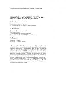
Deriving the corner point flux approximation for an interior node, i.e. a node away from the reactor boundaries, begins by assuming that the diffusion coefficient can be treated as the constant at each point and that value can is a composite average of the diffusion coefficients for the nodes adjacent to said point. The 4-point difference scheme for the Laplacian derived above is used to write two expressions for the current as a function of the corner point flux and either the surface-averaged flux values or the nodeaveraged flux values. Figure 4 shows the two locations where the flux values are chosen. The nodeaveraged flux values correspond to Points 1, 2, and 3, and the surface-averaged flux values correspond to points 1', 2', and 3'. Once these two approximations for the net current are formed the two formulas are subtracted and set to 0, and the solution for the corner point value can be derived from the resulting equation. First, the streaming term Na D is expressed in terms of the node-averaged flux values, and again as Sa in terms of the surface-averaged flux values.
25
Figure 4. Geometry used in construction of the four-point stencil for the corner flux. Applying the first order 4-point stencil derived in the previous section, Na is expressed as
D D2 D3 D11 D22 D33 3 1 3 Na 3 2 a 4
0 ,
107
which simplifies to
Na
D11 D22 D33 D1 D2 D3 0 . 3 2 a 4
108
Using the same method, the equation for Sa is expressed as
D D3 D D4 D1 D2 D D2 D3 1' 2 2 ' 3 3 ' 3 1 2 2 2 3 Sa 2 3a 4 2
0 '
109
which reduces to
Sa
2 D1 D2 1' 2 D2 D3 2 ' 2 D3 D4 3 ' 4 D1 D2 D3 0 ' 3a 4 2
2
26
.
110
Next, taking the difference between Sa and Na , multiplying through by the denominator, and solving for the corner flux 0 , gives the following corner point approximation equation: 3
0
2( D1 D2 )1' 2( D2 D3 )2' 2( D3 D1 )3' Dii i 1
3( D1 D2 D3 )
Oa 3 .
111
This result was first produced by Finnemann, Böer, and Müller5 and it agrees within 4% with the corner point flux approximation produced by Yang, Fink, and Khalil.4 Instead of using an arithmetic average for the diffusion coefficients, flux-weighted or possibly current-weighted averages could also be used.
2.8
Computational Implementation
The methods incorporating the discontinuous terms of the transverse leakage into a hexagonal-z geometry nodal code and described in this Section 2 have been coded into a FORTRAN code and are currently undergoing debugging and testing. This work is ongoing.
27
3.
MODELING BURNABLE POISON RODS IN THE NODAL GREEN’S FUNCTION METHOD FOR THE NEUTRON DIFFUSION IN HEXAGONAL-Z GEOMETRY
The treatment of highly neutron-absorbing rods or burnable poisons (BPs) within the framework of neutron diffusion theory, in particular nodal methods, has historically relied on detailed lattice physics calculations (based on transport theory) and homogenization theory for the generation of equivalent nodal diffusion group constants. The success of this approach rests on the assumption that an accurate representation of the neutron physics within a fuel assembly can be achieved, even if the assembly is separated from surrounding assemblies and simplified boundary conditions are applied to the transport problem. While this assumption remains valid for reactors with a thermal spectrum and small mean-freepaths, such as in the case of light water reactors (LWRs), new reactor concepts and designs may challenge the current paradigm. In particular, the optically-thin graphite-moderated high temperature reactors (HTRs) such as that proposed for the NGNP, may require a multilevel approach that could require special modeling of the BPs, particularly in the case of the prismatic design. A systematic outline of the proposed approaches to modeling HTRs based on neutron diffusion theory has been presented by Ougouag.3 The goal of this work is to propose an explicit treatment of the BP rods located inside homogenized hexagonal nodes, thus incorporating the treatment into nodal hexagonal methods while retaining fidelity in the modeling of the BPs local effects.
3.1
Theory
The treatment of BPs outlined in this report pertains specifically to the graphite-moderated prismatic HTR design. Therefore, this section describes the HTR assembly design and discusses certain salient features regarding the interassembly effects of the BPs. A mathematical model for the absorption behavior due to BP presence is proposed, and the neutron diffusion equation is introduced. The NGFM is then introduced and applied to the diffusion equation, thus arriving at a set of approximate equations for discrete variables that can be readily solved via standard iteration techniques.
3.2
Physics Considerations
The presence of BPs in the prismatic HTR design is intended to counteract power peaking, which occurs at the vertices of the hexagonal fuel assemblies because of the so-called ‘mini-reflector’ effect that arises from the relative higher presence of moderator material.3 Unlike LWRs, the effects from the absorption due to the BP in the prismatic HTR design is felt by neighboring assemblies, thus causing an inter-assembly flux depression. Before accounting for the neutronic effects of the BP over neighboring fuel blocks, the neutron diffusion model must incorporate a correction that preserves the exact transport reaction rate occurring near and inside the strongly absorbing region. This is because diffusion theory fails to achieve sufficient accuracy (with respect to transport theory) near a strongly absorbing medium. The approach incorporated in this work involves the application of the ‘equivalent cross-section method,’ in which the absorption reaction rate from transport theory is precomputed and the diffusion theory-based flux is used to recover the expectedly more accurate transport-based absorption rate. A key aspect in the generation of the BP reaction rates is the determination of the correct diffusion-equivalent flux spectrum from the transport calculation. A particular methodology for generating accurate reaction rates, which relies on the blackness theory hypothesis, is proposed at the end of this report. The next section discusses the mathematical formula for BP treatment within the neutron diffusion equation context and introduces the NGFM.
28
3.2.1
Mathematical Developments
Consider the integrated reaction rate due to absorption occurring inside a finite-dimensional subdomain of volume V p , henceforth referred to as a BP, surrounded by an infinite homogenous material containing a time-independent distributed source that emits monoenergetic neutrons isotropically,
Rap p a r r dV
112
V
where r represents the scalar flux as a function of space, a r is the macroscopic absorption
cross-section for the whole domain, r R 3 , and all other notation, unless otherwise stated, is standard. Under the assumption that the macroscopic absorption cross-section inside the BP is constant, and defining the average flux over the absorbing region in the following manner,
p
1 Vp
V
p
r dV
113
we obtain the reaction rate due to absorption over the BP in terms of the average flux,
Rap apV p p
114
where ap is the constant macroscopic absorption cross-section inside the BP. Any proposed equivalent model for the BP absorption should at least conserve the integrated reaction rate over the subdomain. Next, consider Equation 112 and assume space dependence for the macroscopic absorption rate inside the BP region. In particular, let us define the space-dependent absorption cross-section as
, r r ' p r a r r ' . 0, r r ' p a
115
This representation of the absorption cross-section is clearly a mathematical idealization, since the actual macroscopic cross-section is constant over the burnable absorber. This model for the absorption cross-section will be justified by certain advantages that it brings to the NGFM approach, as shown later in this report. It is clear that, according to Equation 115, the absorption cross section behaves as a Dirac delta function (more accurately, a generalized Dirac product), and that the definition presented in this report is merely heuristic. The proposed model for the absorption cross-section for the BP, which ‘collapses’ the region into a line absorber, can be written as
ap r ap x x ' y y '
116
where x ', y ' indicates the location of the BP, which is assumed to be constant along the z-direction,
X X ' , X x, y is a symbolic function of the delta distribution, and ap is an effective absorption reaction rate that has yet to be determined. In light of Equation 116, the integrated absorption reaction rate is
V BP
ap r r dV ap h p x ', y '
117
29
where h p is the height of the line or collapsed absorber BP and x ', y ' is the z-direction-averaged scalar flux evaluated at the location of the BP. In order to conserve the integral reaction rate, we must enforce the following condition on the BP model:
ap h p x ', y ' apV p p
118
Note that Equation 118 implies that ap must be determined such that the actual absorption reaction rate (right side of the equation) should be recovered when ap is multiplied by the flux at the location of the BP. However, diffusion theory is unable to produce the correct average flux p because this is the averaged flux inside the BP region. Thus, an auxiliary transport calculation must be performed and incorporated into Equation 118 in order to correctly obtain p . The limited applicability of diffusion theory in problems that contain strong neutron-absorbing regions requires the use of transport corrections in order to obtain a more accurate treatment of the particular configuration. Many different methods have been devised (and reported in the relevant literature) that deal with these situations. Examples of such specialized treatments include the response function method and the method of equivalent cross-sections. In the particular case of the equivalent cross-section method, the generation of diffusion group constants is performed based on the recognition that certain linear functionals, such as the average group reaction rates, are theoretically conserved and ideally recovered by the nodal diffusion calculation. A similar approach is incorporated in this work in order to conserve the transport-based absorption reaction rate. Equation 118 is therefore considered and solved for the effective absorption rate
ap ap A p
p
119
x ', y '
where A p is the physical area of the BP in the x, y plane. Note that the z-averaged flux evaluated at the location of the BP has yet to be determined. In fact, this is the quantity that we wish to be computed by the direct diffusion calculation based on a given value for the macroscopic cross-section ap . Since the z-averaged flux is not known a priori, we must precompute the relationship between the averaged flux over the BP and the flux evaluated at the location of the collapsed BP. This situation is worsened by the fact that the averaged flux predicted by diffusion theory will fail to reproduce the transport-based averaged flux. In order to circumvent this drawback the blackness theory hypothesis is leveraged. Blackness Theory predicts the relationship between the transport and diffusion solution near strongly absorbing regions. Therefore, the following developments assume an ‘auxiliary’ transport computation in which the BP is not collapsed as it is in the model presented in the previous subsection. This effort begins by defining the average scalar flux over the absorber region from an auxiliary transport calculation as
trp
1 Vp
V
p
tr r dV .
120
30
Additionally, because of the symmetry of the problem, the dimensionality of the auxiliary transport calculation may be reduced to a single dimension that can be effectively treated in a cylindrical coordinate system. The z-averaged scalar flux can be evaluated at a distance rd from the center of the BP, which is conveniently chosen to coincide with the distance at which the z-averaged scalar flux from diffusion matches the transport solution, i.e.,
tr rd rd
121
The particular distance rd is predicted by blackness theory and is a function of the transport crosssection. Once this ‘equivalence’ distance is determined, the ratio between the average scalar flux for the BP and the equivalent scalar flux at distance rd can be evaluated, which is defined as
Fp
trp
tr rd
.
122
Since the averaged flux over the BP in Equation 119 must be equal to the transport-based averaged flux, we may solve Equation 122 for trp , substitute the resulting expression into Equation 119, and,
under the assumption that x ', y ' tr rd rd , the expression for the effective absorption rate is
ap ap A p F p
123
The expression thus derived accounts for two important assumptions in the treatment of BPs: the modeling of the BP as a collapsed absorbing region that attempts to conserve the physical reaction rate, and the approximation that the flux evaluated at the collapsed location of the absorber is equal to the flux evaluated at the ‘equivalence’ distance as predicted by blackness theory (which for weak transport effects is not expected to be too far away from the BP). In practice, the effective absorption cross sections (reaction rates) will be precomputed by an auxiliary transport calculation and assumed to be constant by the nodal diffusion calculation. However, it is theoretically possible to iterate between the auxiliary transport calculation and the nodal diffusion due to sheer speed of the methodologies and relative simplicity of the treatment. The diffusion theory model is introduced and the NGFM approach applied. The steady-state multigroup, multidimensional neutron diffusion equation for a homogenous hexagonal node V k is
Dgk 2 gk r rk, g r gk r Qgk r
124
where
Qgk r F gk ' r
125
and
g F k
G
g '1
k f ,g '
ks , gg ' g ' g
126
31
where Dgk is the direction-independent diffusion coefficient, and kr , g r , kf , g ' , and ks, gg ' are the removal, fission, and scattering macroscopic cross sections, respectively. In addition, g is the fission spectrum and k is the effective multiplication factor. Note that the removal cross-section is spacedependent within the node and reduces to the absorption cross section for the particular case of a single energy group ( G 1 ). Note that the removal term on the left side of Equation 124 is space-dependent and involves P 1
terms, where P denotes the total number of BP rods inside node k , i.e., kr , g r kr , g By operating over this removal term in the diffusion equation with
1 Vk
dV
V
P
r . p 1
k, p r,g
and introducing the model
k
for the BP rod defined by Equation 116, there results
1 Vk
1 k k k k k r , g r g r dV r , g g V k V
where x p , y p
P
p 1
denotes the location of the
gk , p x p , y p
k, p r,g
127
p th BP pin. Finally, the neutron balance equation in
hexagonal geometry is reached:
1 k 1 1 Lgz Lkgu Lkgv Lkgw rk, g gk k 2a 3h V
P
p 1
gk , p x p , y p Qgk .
k, p r,g
128
The transverse-averaged ordinary differential equation, resulting from the transverse-integration procedure and averaging of Equation 124, is
d2 k D gx x rg,k gxk x Q gxk x Lkgx x 2 dx k g
129
where the transverse-averaged leakage is defined as
1 1 J gk , z x, ys x J gk , z x, ys x J gk , y x, a J gk , y x, a 2 a 3 ys x
Lkgx x
ys' x d k , z d d g x, ys x gk , z x, ys x 4 gxk x D dx dx 2 ys x dx k g
130
ys'' x gk , z x, ys x gk , z x, ys x 2 gxk x D 2 ys x k g
In order to solve the ordinary differential equation described above, the Green’s function solution for the 1-D elliptic operator is obtained, thus yielding the solution
h
k gx
xo h
x dxo Ggxk x | xo S gxk xo Ggxk x | xo J gxk xo x h o
h
32
131
The Green’s function moment is the integral of the product of Green’s function and the an element in the orthonormal expansion coefficients basis as
Gglk x
h
dx
o
h
Ggxk x | xo Bl xo .
132
The ‘sink’ term arising from the presence of BPs is evaluated according to
Ggxk x | x p xo x p k , p k k p k,p k p p h dxo Ggx x | xo 2 ys xo r , g g xo , y 2 ys x p r , g g x , y h
133
into which, for convenience, the notation
G
k, p g
x
Ggxk x | x p 2 ys x p
,
134
is introduced. With the above definitions and notations, the Green’s function solution to the 1-D transverse-averaged diffusion equation becomes 2
P
l 0
p 1
k gxk x S gxl Gglk x Ggk , p x rk ,,gp gk x p , y p Ggxk x | xo J gxk xo . x h xo h
135
o
The standard approach for solving the set of NGFM equations involves the standard inner/outer iterations in which an initial guess for the flux solution is assumed (set of spatial moments for all directions) and the effective multiplication factor is initially take to be unity. The inner iterations involve a directional sweep followed by an update of the transverse-leakage terms. Once the net currents for all dimensions are updated, the moments of the direction flux solution is updated and the upscattering/downscattering contributions are computed. the treatment of the BPs in the context of the Green’s function solution requires the reconstruction of a 2-D flux shape based on sets of linear functionals obtained from a direct calculation. The particular method proposed in this work involved the use of the directional spatial moments of the flux to reconstruct the flux and evaluate the expression at the BP location. While other more accurate methods exist and are routinely used for reconstruction, it was found that a low-order 2-D quadratic polynomial provides all the features necessary to the implementation of a ‘proof-of-principle’ for the methodology.
3.3
Numerical Results
Some numerical results from simple tests that were selected in order to test the implementation of the BP treatment are reviewed in this section. A stand-alone nodal hexagonal NGFM-based code was modified in order to incorporate the treatment presented in this report. The results that are included are based on the ‘manufactured solution’ approach. In this approach a specific solution is chosen a-priori then a problem is constructed the solution of which is that a-priori selected one. This process allows an effective test of the implementation of the method. The numerical results are expected to reproduce the known solution within “reasonable” tolerance levels ranging from machine precision level for some problems to the systematic error level of the Green’s function method. A large discrepancy would
33
provide symptoms of problems to be corrected. A particular problem configuration in order to validate the approach is also proposed.
3.3.1
Manufactured Problems
In order to verify that the methodology has been implemented correctly, a set of manufactured solutions must be defined in such a way that they exercise the parts of the code that have yet to be tested. For these purposes, a manufactured problem involving a single hexagonal node with reflective boundary conditions and a distributed fixed source is proposed. For the sake of simplicity, it is assumed that the problem is monoenergetic and fictitious group diffusion constants are selected as shown in Table 1. Table 1. Physical parameters for manufactured problems.
D 1.5cm
Q0 1
r 0.02cm 1
Q0 0.1
2h 10cm
Q0 0.1
The manufactured solution based on the constraints outlined above is 2
x Ql Gl x l 0
G p x
136
2 ys x p
where kr ,,gp is chosen so that kr ,,gp gk x p , y p 1 and only a single BP is present inside the hexagonal node at a specified location. Four different locations are chosen with respect to the u-direction, as shown in Table 2. Table 2. BP Location for manufactured problems (all dimensions in cm). Case Number 1 2 3 4 5
up
vp
wp
0.0 2.5 -2.5 5.0 -5.0
0.0 -1.25 1.25 -2.5 2.5
0.0 1.25 -1.25 2.5 -2.5
The quantities used to compare the computational results against the reference solutions were the value of the 1-D flux at x h , 2
h Ql Gl h l 0
G p h
137
2 ys x p
and the projection of BP contribution to the solution over the set of orthonormal polynomials Bl ' x ,
l '
1 2 3h 2
h
dx2 ys x Bl ' x
h
G p x
2 ys x p
.
138
34
The results from this comparison for the manufactured problem, shown in the Tables 3, 4, and 5, indicate that the implementation is able to reproduce the reference values for the quantities defined by Equations 137 and 138 up to single precision finite arithmetic. The cause for some of the variations in the difference between the reference values and the numerical values may be the fact that the exact values were obtained from a FORTRAN calculation, in which the implementation is written in, while the reference values were not. Generally speaking, single precision agreement seems to indicate correct implementation of the methodology.
Table 3. Manufactured problem results for the u-direction solution. error Location (x=0) error Sbp0 7.84145E-09 phi(+h) 1.10769E-07 Sbp1 1.35093E-16 phi(-h) 6.75399E-08 Sbp2 6.15609E-10 error Location (x=h/2) error Sbp0 1.03624E-08 phi(+h) 1.83101E-07 Sbp1 2.38905E-09 phi(-h) 1.94140E-07 Sbp2 1.82636E-11 error Location (x=-h/2) error Sbp0 1.03624E-08 phi(+h) 2.96773E-07 Sbp1 2.38905E-09 phi(-h) 2.57941E-07 Sbp2 1.82635E-11
Table 4. Manufactured problem results for the v-direction solution. error Location (x=0) error Sbp0 7.84145E-09 phi(+h) 1.10769E-07 Sbp1 1.35093E-16 phi(-h) 6.75399E-08 Sbp2 6.15609E-10 error Location (x=h/2) error Sbp0 8.93674E-09 phi(+h) 1.90925E-07 Sbp1 1.11686E-09 phi(-h) 1.24611E-07 Sbp2 5.0225E-10 error Location (x=-h/2) error Sbp0 8.93674E-09 phi(+h) 1.88835E-07 Sbp1 1.11686E-09 phi(-h) 2.66521E-07 Sbp2 5.02258E-10
35
Table 5. Manufactured problem results for the w-direction solution. error Location (x=0) error Sbp0 7.84145E-09 phi(+h) 1.10769E-07 Sbp1 1.35093E-16 phi(-h) 6.75399E-08 Sbp2 6.15609E-10 error Location (x=h/2) error Sbp0 8.93674E-09 phi(+h) 1.68834E-07 Sbp1 1.11686E-09 phi(-h) 1.48851E-07 Sbp2 5.02258E-10 error Location (x=-h/2) error Sbp0 8.93674E-09 phi(+h) 2.24328E-07 Sbp1 1.11686E-09 phi(-h) 2.32956E-07 Sbp2 5.0225E-10
3.3.2
Proposed Model Problem
The previous subsection proposes a set of manufactured problems that were used to test the implementation of the methodology. While this shows that in fact, the set of equations derived in this work have been correctly implemented, the BP treatment still requires validation against higher fidelity calculations. In order to do this, a simple 2-D one-group single-node problem is proposed that can be readily solved using transport theory computational tools in a tractable amount of time. A short description of the proposed problem is presented here. In order to isolate the complex effects that geometric detail, cross-section energy condensation, and spatial homogenization add when comparing a nodal diffusion solution to a fine-mesh transport theory solution, a simple single-node problem is proposed with a BP pin located in the coordinate center of the hexagon and with reflective boundary conditions applied throughout the boundary (six faces). This problem configuration is equivalent (or at least very similar) to the conceptual framework used to derive the BP treatment and equivalent cross-section method in Section 3.2. The BP is surrounded by a fuel region that is equivalent to a mixture of HTR fuel compact and graphite moderator materials. A set of fictitious cross sections will be manufactured that will test the accuracy of the method parametrically (effective multiplication factor and flux distribution) as a function of fuel and absorber size as measured in mean-free-paths. This proposed model problem, while simple, will allow the avoidance of other more complex effects that may skew the validation of the BP treatment. In addition, more sophisticated physics can be hierarchically added to this problem until a more realistic configuration is achieved.
3.4
Final Assessment of Burnable Poison Model
This report outlines a novel treatment for BPs in hexagonal geometry under the assumption of neutron diffusion theory. Particularly, the Nodal Green’s Function Method approach for solving the diffusion equation is adopted because it allows for the solution of even complicated source shapes, well beyond low-order polynomials. This is especially warranted in this case, because local intra-assembly BPs are modeled as delta distributions, thus requiring special treatment. The model of BPs as delta distributions rather than smeared materials is motivated by the physical observation that in optically thin, graphitemoderated HTRs, BPs can affect neighboring assemblies and thus produce an inter-assembly effect that is uncharacteristic of other reactor types (such as LWRs). The treatment of the BP as a delta distribution is constrained by imposing conservation of the physical absorption reaction rate as obtained from an auxiliary transport calculation. The blackness theory hypothesis is subsequently used to relate the 36
diffusion theory-based flux evaluated at the BP location and the transport reaction rate due to absorption caused by the BP.
4.
SUMMARY STATUS OF CODE DEVELOPMENT
This report presented the recent developments on two topics. The first topic was the development of a method that accounts explicitly for singular and discontinuous terms in the transverse leakage of nodal methods that arise from the transverse integration procedure in hexagonal geometry. The method has been developed and supporting mathematical tools have been devised. The method was implemented into a FORTRAN code that is undergoing debugging and testing. The second topic was the development of a method for the explicit treatment of burnable poisons without their homogenization into the prismatic fuel blocks (equivalent of assemblies) in order to preserve their localized effect in the model. The mathematical formulation of the new method has been completed and the method has been implemented in a FORTRAN code. The code was verified using the method of manufactured solutions and shown to have been implemented correctly. The code must still be validated by comparison to reference transport theory data. The generation of transport theory data was not within the scope of the project this fiscal year. The project is leveraging a companion project (Deep Burn Project) in which the transport-theory-based reference reaction rates in which the needed auxiliary data are to be developed. Those data are not yet available. A similar methodology for development of auxiliary data is to be pursued at the INL next fiscal year. Work is also currently underway to test the results against transport solutions.
5.
REFERENCES
1. R. D. Lawrence, The DIF3D Nodal Neutronics Option for Two- and Three-Dimensional
Diffusion Theory Calculations in Hexagonal Geometry, ANL-83-1, 1983. 2. M. R. Wagner, “Three-dimensional nodal diffusion and transport theory methods for
hexagonal-z geometry, Nucl. Sci. Eng., Vol. 103, 1989, p. 377. 3. A. M. Ougouag, Systematics of Neutron Diffusion Modeling for Neutron-Optically Thin,
Multiply-Heterogeneous High Temperature Reactors, Idaho National Laboratory, INL/EXT-09-16414, July 2009. 4. W. S. Yang, P. J. Finck, and H. Khalil, “Reconstruction of Pin Power and Burnup
Characteristics Form nodal Calculations in Hexagonal-z Geometry,” Nuclear Science and Engineering, Vol. 111, 1992, pp. 21–33. 5. H. Finnermann, R. Böer, and R. Müller, “Combination of finite-difference and finite-volume
techniques in global reactor calculation.” Kerntechnik, Vol. 57, No. 4, 1992, p.216–222. 6. W. Firzpatrick, Developments in Nodal Reactor Analysis for Hexagonal Geometry. PhD
Thesis Universtity of Illinois at Urbana-Champaign, 1995.
37