Noise Level Estimation for Digital Images Using Local

TELKOMNIKA, Vol.16, No.2, April 2018, pp. 915~924 ISSN: 1693-6930, accredited A by DIKTI, Decree No: 58/DIKTI/Kep/2013 DOI: 10.12928/TELKOMNIKA.v16i2.9060

 915

Noise Level Estimation for Digital Images Using Local Statistics and Its Applications to Noise Removal 1

1,2

2

3

Asem Khmag* , Sami Ghoul , Syed Abdul Rahman Al-Haddad , 4 Noraziahtulhidayu Kamarudin Computer system Engineering, Faculty of Engineering, Univers ity of Zawia, Az zawia, Libya Computer & Communication Engineering, Universiti Putra Malaysia, Serdang, Malayisa *Corresponding author, e-mail: [email protected], [email protected]

3,4

Abstract In this paper, an automatic estimation of additive white Gaussian noise technique is proposed. This technique is b uilt according to the local statistics of Gaussian noise. In the field of digital signal processing, estimation of the noise is considered as pivotal process that many signal processing tasks relies on. The main aim of this paper is to design a patch-b ased estimation technique in order to estimate the noise level in natural images and use it in b lind image removal technique. The estimation processes is utilized selected patches which is most contaminated sub -pixels in the tested images sing principal component analysis (PCA). The performance of the suggested noise level estimation technique is shown its superior to state of the art noise estimation and noise removal algorithms, the proposed algorithm produces the b est performance in most cases compared with the investigated techniques in terms of PSNR, IQI and the visual perception. Keywords: Additive noise, noise estimation, principal components a nalysis, patch selection, image denoising. Copyright © 2018 Universitas Ahmad Dahlan. All rights reserved.

1. Introduction The estimation of noise models has its significant impact in several applications such as computer vision, pattern recognition, image segmentation and registration, to name a few. In the field of image processing techniques, we need to know in most of the time the amount of noise before we involve in any process such s image restoration, object moving detection and image enhancement, etc. In this regard, image noise removal plays a vital role when it comes to the issue of increasing the quality of the appearance of the noisy images and make more pleasant in human perception. In field of image processing, noise level is a crucial parameter that can affect numerous subjects of study, such as denoising, segmentation, super-resolution, deblurring, and registration [1]-[2]. One of the pioneer’s image analysis techniques tool which utilizes wavelet domain is quaternion wavelet transform. It uses the shift -invariant feature that the coefficients are localized in time and frequency domains to provide full information about the image texture and fine details In study that conducted by Chan in [3], the notion of (DTCW) is extended to the quaternion transformation by exploiting conceptions of 2D Hilbert domain in order to analysis the signal with the application to disparity assessments. Theoretically, quaternion wavelet transform is used widely in the field of image noise removal [4]-[5], classification of deep details [6]-[7], deblurring and its applications [8] and computer fusion [9]. In [10], a novel generalized signal-dependent for noise model is designed in natural images which acquired using a digital camera. In their method, Gamma factor is estimated for more efficient estimation. Another s tudy utilized an automatic noise estimation technique based on local statistics to remove Additive Gaussian noise [11]. They managed to process multiplicative Gaussian noise and achieved high visual performance and fast execution time. In study which was done by [12], a discrete-time learning algorithm in order to restore fast a contaminated image using a novel L2-norm noise estimation. In their method, the suggested technique conquers the difficulties of noise estimation methods such as false estimation which is appear in CNF algorithm. A framework design for block -based approaches that combine the strengths of different filters is presented in [13]. The identifying of the homogeneous blocks is Received November 5, 2017; Revised February 19, 2018; Accepted March 12, 2018

916



ISSN: 1693-6930

utilized in order to evaluate its performances with state of the art methods. The complexity of noise filtering was reduced tremendously but the visual quality performance was slightly improved. Noise discrepancies in multiple scales are utilized in [14]. It is implemented as indicators for the detection of image splicing forgery. The test images are initially segmented into patches (sub-pixels) for different levels, the noise is studied in every single level adaptively. Furthermore, in [15], an efficient approach was proposed in order to estimate the noise level with precise rate in wavelet domain. They found out that the variance sum of high frequency components in the contaminated coefficients of quaternion wavelet is mainly equal to the noise amount. However, they suffered from fault estimation especially in high noise levels. In addition, a novel and efficient noise level estimation technique is proposed in [16], also they analyze the change of singular values in order to determine the content related parameter, and they applied their technique on different kinds of images. The rest of this study is prepared as follows. Assessment of noise using Principal Component Analysis (PCA) is explained in Section 2. The proposed noise level estimation is demonstrated in Section 3. The blind noise removal from natural images algorithm is discussed in Section 4. Extensive experiments and its results are presented in Section 5. Finally, the conclusion is stated in Section 6.

2. Research Estimation of Noise Levels Using PCA Noise level estimation in patch-based noise models utilizes a specific of patches or subimages in order to derive it from the noisy counterparts. In this paper, the proposed algorithm applied the windowing technique for every single patch and then slide pixel -by-pixel until the whole investigated image is completely covered. The formula of each contaminated patch can be written by: (1) where N represents each patch number; ni is the index of each patch and the patch size is represented by M x M , where the sub-images is defined by its central pixel; zi denotes the observed noisy patch by independent noise model (Inpendent and and Identically Distributed iid). The additive Gaussian noise (AWGN) model denoted by ni with zero mean and variance Additionally, the noise models of the intersected patch pairs reflect a kind of correlation. However, non-overlapping sub-image pairs in most of time occur in the whole patches. In order to clarify the overlapping process, the noise modes are presumed to be independent completely in the whole tested patches. The input noisy patches are stated as dataset in Euclidean models. Furthermore, the orientation of the axis can be defined using the unit vector u. In harmony with the up mentioned assumption that the noisy image has a uncorrelated behavior, accordingly, the variance of the projected noisy image details can be found by: ,

(2)

where V(uTxi) represents the variance of the patches that indicated by in the directions; and σn is the standard deviation of noise model, umin is the minimum direction variance that can be found using (3) In the same regard, in [17], the maximum variance is computed using PCA in order to find the correlation amomng the sub-pixels. The eigenvector is utilized in this study in order to find the lowest variance orientation and also it exploits the minimum eigenvalue to bui ld its covariance matrix, it is found using the following expression: ( )

TELKOMNIKA Vol. 16, No. 2, April 2018 : 915 – 924

(4)

TELKOMNIKA

ISSN: 1693-6930



917

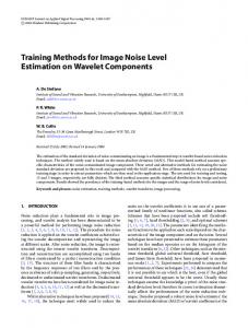
is the noise-free signal. The variance of the desired patches, which is found along the minimum variance direction, is normally identical with the minimum eigenvalue of covariance medium. As a result, the calculation of variance direction is used to find out the covariance matrix and its related eigenvalue. (5) depicted the covariance matrix of contaminated sub-image represents the covariance matrix of the original sub-image (patches), and represents the lowest eigenvalue of matrix . The analysis of the lowest eigenvalue of the covariance matrix of the noisy patches is represented in (5). Furthermore, the model of AWGN is found accordingly. On the other hand, this decomposition issue is an ill-posed issue due to the lowest eigenvalue of the covariance array of the original sub-image is unavailable. Although the clear disadvantage of this matter, the digital images features can be utilized to estimate the noise level. The repeated textures and its pattern in natural images can be used as the main source of the image features. Additionally, the structures of natural images span only low-dimensional structure. When the details of each sub-image span a sub-space with dimensions that have size less than , then those sub-images are determined by the term low-rank sub-image (patch). In the same regard, ) which denotes to slightest eigenvalue of the covariance matrix is assumed to be ignored due to insignificant effect. From theoretical point of view, the AWGN model reflects the same power spectrum in every path in the contaminated image, and as a result, all its eigenvalues will show the same value along with their power spectrum. In this step, noise level can be estimated consequently by utilizing the sub-space spanned over the eigenvectors of the covariance matrix that carries nil eigenvalues as represented by the following formula: (6) Theoretically, the hypothesis of the redundancy is not necessarily correct, but from practical point of view, it will work in digital images arena which contain rich details and full of complicated textures and repeated patterns. In order to discuss the proposed PCA -based noise level estimation results, two examples have been depicted. The Boat in Figure 1 depicts a kind of simple image details and fine textures. In this case, the low-rank patches is very clear, patches which have mostly lines and symmetrical shapes. The smallest eigenvalue of the benchmark Boat image in this case is approximately zero. Consequently, the suggested PCA based approach can completely estimate the noise model levels, as shown in Figure 1. On the other hand, Figure 2 depicts the benchmark image Fingerprint. In this scene, the target image reveals kind of complicated textures, fine details, rich and repeated edges. The minimum eigenvalue of the sub-pixels in Fingerprint has values which are larger than zero. As a result, the suggested technique overestimates the noise level; this can be justified due to the noise level and amount of complicated texture inside the target noise image low noise scale. Table 1 and 2 depicts the ground truth and estimated noise levels in both benchmark images it can be clearly notice that there is very strong correlation among the patches in Boat image rather than Fingerprint image that consists of too many rich textures, which the proposed algorithm visibly overestimates the noise level.

3. Patch Selection Approach Currently, the two pivotal issues of the noise assessment approach are elaborated: the selection of single patch and iterative framework for noise level assessment. Sub-images and patches based image noise assessment techniques depend on the contaminated image and its noise model. The noisy image is categorized to a set of patches in a raster scan model according to its geometric configuration. In order to find the appropriate sub-images and select them from their contaminated images, it is necessary to investigate the imae details and its configuration. Homogenous patches is utilized and stated in Lee and Hoppel [18]. In their method, the patches which reflect the smallest variance homogenous is used as a feature in the noisy image. In study which was conducted by Khmag et al [19] gave out an approach in order Noise Level Estimation for Digital Images Using Local … (Asem Khmag)

918



ISSN: 1693-6930

to estimate AWGN using PCA and correlated patches which have complicated structures, where patches with large variances are disregarded. Despite CPU time friendly of the proposed method, it shows an overestimate noise levels in images that contain lots of complicated textures. In order to improve the previous technique, a study which done by Shin et al. [20] that modified their technique by exploiting an adaptive threshold amount that used in patch variance to select the specific contaminated patches. However, the selected patches still far away to be considered as an ideal choice due to the complicated texture of the majority digital natural images. In this paper, texture strength metric is introduced. It is organized based on the Matrix of source digital image gradients and its local statistical features to select the low-rank set of the investigated sub-images. Furthermore, a noise removal approach is introduced to utilize the noise estimation model proposed in this study. Zhu and Milanfar [21] exploited the gradient covariance matrix in order to use it as a measurement balance to manipulate the image structure. In this regard, a contaminated digital natural image patch yi has size of N2×2 of the gradient matrix is formulated as follows: (7) Where Dh and Dv are the horizontal and vertical derivative operator matrices, respectively. Dh and Dv are Toeplitz matrices with size [22], which are resulted from a gradient filter. In addition, the covariance matrix gradient C of contaminated sub-image is found as C =C

T

G

(8)

Accordingly, =

D D

where is the mathematically operator transpose. The gradient matrix G and the gradient covariance matrix C have the greatest noisy image patches information, statistical behavior and their structure details. The eigenvectors and eigenvalues of C are exploited in order to compute the main direction and its power [23].

Table 1. Proposed Noise Model Assessment Method and Round Truth Estimation of Fingerprint Noise Level 0 5 10 15 20 25 30 35 40 45 50

Ground Truth 0 5 10 15 20 25 30 35 40 45 50

Estimated Noise 0 4.6 10.02 15.07 20 24.6 30 35.6 40.8 45.2 50.1

Figure 1. Benchmark image of Fingerprint

TELKOMNIKA Vol. 16, No. 2, April 2018 : 915 – 924

TELKOMNIKA

ISSN: 1693-6930



Table 2. Proposed Noise Model Assessment Method and Round Truth Estimation of Noise Level 0 5 10 15 20 25 30 35 40 45 50

Ground Truth 0 5 10 15 20 25 30 35 40 45 50

919

Boat

Estimated Noise 12 17 20 23 28 32 37 40 44 48 53

Figure 2. Benchmark image of Boat

The fine textures and fine details reflect how much the tested patch is strength, it comes from aggregation of the whole eigenvalue components of the investigated covariance matrix. In addition, a strength patches reflect the full texture details. Consequently, the strength of the texture that represented by η is computed by (10) where tr(.) depicts the thresholding operator. Low-rank sub-images which contain sharp ridges modules in noise-free images are mostly considered minor and as a result it can be certainly divided by applying thresholding technique on the tested texture. However, the gradient textures are very sensitive to high noise levels, and thus, the texture strength performance will be effected by sever noise levels. As a result, Gaussian noise performance with texture strength might be further stated. Regarding, the noisy patch has kind of flat manner, the impeccably flat patch and its relative gradient matrix G is expressed as G

(11)

The noisy flat sub-image that represented by yf in additive noise model can be written as (12) In this regard, n denotes to the additive noise model sub-image and it has standard deviation . As shown in (11), the gradient of the flat sub-image can be represented by zero, whereas the gradient matrix of the contaminated sub-image is found be the following formula:

(13) 3.1. Blind image noise removal algorithm The proposed method for blind image restoration is introduced according to discrete wavelet transform (UWT) which is applied with PCA technique. As shown in Figure 3, the proposed method consists of two main parts. It is started with the noisy image that is found by Noise Level Estimation for Digital Images Using Local … (Asem Khmag)

920



ISSN: 1693-6930

adding Gaussian noise model to the original natural images, then by eliminating the majority of the noise through the application of DWT and PCA. The other part is started with applying semisoft thresholding approach to remove the noisy coefficients in order to kill the coefficients that carry most of low frequency components that resulted from Gaussian noise. The inverse discrete wavelet transform (IDWT) is lastly applied in order to attain the full recovered image. The last step before the resulted image can be attained is to resume the original specifications of the noise-free image such as image format and its size.

Figure 3. Block diagram of the proposed algorithm

4. Results and Discussions In this part, the proposed noise removal technique is tested on 8 well-known images as depicted in Figure 4. The tested benchmark images were used in this study and has been taken from USC-SIPI image database [23], with 180 images in the data sets LIVE [24], TID2008 [25], CSIQ [26], and test in BSDS500 [27]. The resolutions of the tested images were and 481×320, correspondingly. The tested images was contaminated with zero-mean AWGN in different levels of noise, σ = 10, 20, 30, 40, 50, 60, and 7. The overall of 180 simulations are applied for fair assessment to each benchmark image under several noise levels. Furthermore, overlapping sub-image was used in the suggested method. In this study, an extensive comparisons have been conducted with best of state of the art denoising techniques , such as ant colony optimization (ACO) [27], singular value decomposition (SVD) [28], Wiener filter [29], block matching 3D (BM3D) [30], HMM [31] and Ref [11], with their ideal factors that were presented in their original papers.

Figure 4. Eight tested image with size 512 × 512.Upper row: Hill, Peppers, Boat, and Fingerprint. Lower row: Barbara, Military Base, Flinstones, and Tank TELKOMNIKA Vol. 16, No. 2, April 2018 : 915 – 924

TELKOMNIKA



ISSN: 1693-6930

921

4.1 Performance assessments of the noise estimation algorithm Three main factors were taken into consideration when it comes to the issue of noise estimation performance; these factors are estimation precision, consistency, and the overall output of the proposed technique [32, 33]. In addition, average error estimation and noise variance are the mainly factors that mostly exploited to calculate the noise estimation precision and its consistency, they can be computed as follows: M

j

(14)

µE =(1/N) ∑j=1 Ek ,

(15)

Ek =(1/M) ∑j=1 │σ -σ│ N

σ

2 E

N

2

=(1/N) ∑j=1 (Ek -µE)

j

(16) th

th

σ represents the variance which is estimated from j level; Ek is the k error in estimated tested image; and are the images which are included in every testing processes and for each level in AWGN model, respectively. In addition, general performance of the proposed technique is calculated using the following formula: √

(17)

In order to achieve efficient noise model estimation, the values and might be small. Tables 3 and 4 depict comparison results of precision and consistency performance. 4.2 Image denoising results In this section, different noise removal methods have been tested and demonstrated. The main aim in this part of the paper is to show how accurate noise estimation can increase the removal of the noise significantly. From subjective point of view, the quality of the retrieved images was assessed according to peak signal-to-noise ratio (PSNR) which is calculated as follows 2

PSNR=10.log10 (255 /MSE).

(18)

In addition, another subjective assessment is used in this study which is image quality index (IQI). It was applied on the tested images in order to evaluate the how much the reconstructed image is closer to the original counterpart. Image Q-index (IQI) evaluation has a range of (-1, 1). Close value to zero, high visual quality image is achieved; the Q-index model formula can be calculated as follows ̅̅ ̅

̅

(19)

The cross variance σxy is utilized to find the correlation between the noise-free image (x) and the reconstructed image (y); ̅ and ̅ represent the average of the noise-free image and denoised images, correspondingly; and σx2 and σy2 depict the variances of the original and reconstructed images as well [36]. Practically, PSNR graph is shown in F igure 5, this graph shows the benchmark image of Boat, the highest PSNR is reflected in the proposed algorithm. Its highest value is within the range of 0.3–1.2 dB, which is higher than Ref [11] and BM3D. The Wiener2 and SVD filters have the lowest PSNR among the noise removal techniques. Furthermore, Figure 6 depicts the Q-index chart of the different state of the art denoising algorithms for the Boat benchmark image. The proposed technique shows the highest IQI, which is 0.943 to 0.642 in low noise levels respectively. Finally, Wiener2 and ACO algorithms shows the lowest IQI values which were in the range of 0.33 in low noise levels and 0.51 to 0.46 in low and high noise levels respectively.

Noise Level Estimation for Digital Images Using Local … (Asem Khmag)

922



ISSN: 1693-6930 Table 3. Comparison of Noise Level Denoising Method ACO SVD Wiener BM3D Ref[11] HMM Proposed Method

10 1.23 1.44 0.29 0.23 0.32 0.92 0.32

20 0.85 1.40 0.23 0.20 0.25 0.86 0.25

In Several Denoising Filters 30 0.62 1.46 0.20 0.30 0.20 0.83 0.20

40 0.48 1.78 0.18 0.41 0.17 0.76 0.17

50 0.53 2.71 0.17 0.38 0.19 0.69 0.21

60 0.51 2.73 0.12 0.42 0.21 0.73 0.27

70 0.42 2.61 0.18 0.39 0.22 0.78 0.32

Table 4. Comparison of σE In Several Denoising Filters Noise Level Denoising Method ACO SVD Wiener BM3D Ref[11] HMM Proposed Method

10 0.68 0.92 0.60 1.22 3.83 1.02 0.60

20 0.37 0.33 0.50 0.93 2.56 0.87 0.50

30 0.29 0.23 0.32 0.92 1.95 0.81 0.32

40 0.23 0.20 0.25 0.86 1.33 0.78 0.25

50 0.20 0.30 0.20 0.83 1.13 0.77 0.20

60 0.18 0.41 0.17 0.76 1.02 0.71 0.17

70 0.17 0.38 0.19 0.69 0.99 0.68 0.21

Figure 5. PSNR of different filter types with varying noise levels ( ) for the benchmark image Boat

Figure 6. IQI of different filter types with varying noise levels ( ) for the benchmark image Boat

TELKOMNIKA Vol. 16, No. 2, April 2018 : 915 – 924

TELKOMNIKA

ISSN: 1693-6930



923

5. Conclusion Practical noise estimation and its application in image noise removal were discussed and stated in this paper accordingly. The proposed algorithm which is based on PCA approach was utilized with discrete wavelet transformation in order to reduce the dimensionality of the noisy image which is selected from the sub-images. An algorithm to pick out low-rank patches was proposed without choosing the high-frequency components that carry most of AWGN coefficients PCA approach utilized the eigenvalues of the covariance matrix of the noisy image in order to increase the texture strength. The results from the extensive experiments demonstrated that the real level of noise provided the perfect noise reduction performance among most of best state of the art denoising techniques. Regarding to the noise removal of the proposed algorithm, it showed competitive results in most cases compared to state-of-art denoising algorithms in terms of PSNR, image Q-index, and visual perception. As future work, it would be such improvement to the proposed algorithm when different kinds of images such as medical and hyperspectral images are taken as target images in order to remove salt & pepper and shot noise from those tested image

References [1]. Dabov K, Foi A, Katkovnik V, and Egiazarian K. Image Denoising by Sparse 3 -D Transform-domain

Collaborative Filtering. IEEE Transactions on image processing. 2007; 16(8): 2080-2095. [2]. Gilboa G, Sochen N, and Zeevi Y. Estimation of Optimal PDE-based Denoising in The SNR Sense.

IEEE Transactions on Image Processing. 2006; 15(8): 2269-2280. [3]. Chan W, Choi L, and Baraniuk R. Coherent Multiscale Image Processing Using Dual-tree Quaternion

Wavelets. IEEE Transactions on Image Processing. 2008; 17(7): 1069-1082. [4]. Gai S, Yang G, Wan M, and Wng L. Hidden Markov Tree Model of Images Using Quaternion Wavelet

Transform. Computers & Electrical Engineering Journal. 2014; 40(3): 819-832. [5]. Khmag, A., Ramli, A. R., Al-Haddad, S. A. R., & Hashim, S. J. B.. Additive and Multiplicative Noise

Removal Based on Adaptive Wavelet Transformation Using Cycle Spinning. American Journal of Applied Sciences. 2014;11(2): 316. [6]. Gai S, Yang G, and Zhang S. Multiscale Texture Classification Using Reduced Quaternion Wavelet Transform. AEU-International Journal of Electronics and Communications.2013; 67(3): 233-241. [7]. Li C, Li J, and Fu B. Magnitude-phase of Quaternion Wavelet Transform for Texture Representation Using Multilevel Copula. IEEE Signal Processing Letters. 2013; 20(8): 799-802. [8]. Liu Y, Jin J, Wang Q, Shen Y, and Dong X. Region Level Based Multi -focus Image Fusion Using Quaternion Wavelet and Normalized Cut. Signal Processing. 2014; 97(5): 9-30. [9]. Khmag A, Ramli A, Al-haddad S, Yusoff S, and Kamarudin N, Denoising of Natural Images Through Robust Wavelet Thresholding and Genetic Programming. The Visual Computer. 2016; 33(9): 11411154. [10]. Thai F, Retraint A, and Cogranne R. Generalized Signal-dependent Noise Model and Parameter Estimation for Natural Images. Signal Processing. 2015; 114(5): 164-170. [11]. Jiang P, and Zhang J. Fast and Reliable Noise Level Estimation Based on Local Statistic. Pattern Recognition Letters.2016; 78(8): 8-13. [12]. Xia Y, Leung H, and Kamel M. A Discrete-time Learning Algorithm for Image Restoration Using a Novel L 2-norm Noise Constrained Estimation. Neurocomputing. 2016; 198(12):155-170. [13]. Khmag A, Ramli A, Hashim S, and Al‐haddad S. Additive Noise Reduction in Natural Images using Second‐generation Wavelet Transform Hidden Markov Models. IEEJ Transactions on Electrical and Electronic Engineering. 2016; 3(11): 339-347, 2016. [14]. Liu Y, Du W, Jin J, Wang H, and Liang R. Boost Image Denoising Via Noise Level Estimation in Quaternion Wavelet Domain. AEU-International Journal of Electronics and Communications. 2016; 70(5): 584-591. [15]. Ren J, Lu H, and Zeng X. Image Denoising Based on K-means Singular Value Decomposition. TELKOMNIKA (Telecommunication Computing Electronics and Control). 2015; 13(4): 1312-1318 [16]. Chaitanya S. Noise Removal in Microarray Images using Variational Mode Decomposition Technique. TELKOMNIKA (Telecommunication Computing Electronics and Control), 2017; 15(4). [17]. Lee J, and Hoppel K. Noise Modeling and Estimation of Remotely-sensed Images. Symposium in Geoscience and Remote Sensing, 12th IEEE Canadian Symposium on Remote Sensing. Vancouver, Canada, 10–14 July 1989, volume 2: 1005–1008. [18]. Pyatykh S, Hesser J, and Zheng L. Image Noise Level Estimation by Principal Component Analysis. IEEE transactions on image processing. 2013; 22(2): 687-699. [19]. Khmag A, Ramli A, Al-haddad S, and Kamarudin N. Natural Image Noise Level Estimation Based on Local Statistics for Blind Noise Reduction. The Visual Computer.2017; 12(8):1-13.

Noise Level Estimation for Digital Images Using Local … (Asem Khmag)

924



ISSN: 1693-6930

[20]. Zhu X and Milanfar P. Automatic Parameter Selection for Denoising Algorithms Using A no -reference

Measure of Image Content. IEEE Transactions on Image Processing. 2010; 19(12): 3116-3132. [21]. Wang J & Zhang D. Image Denoising Based on Artificial Be e Colony and BP Neural

Network. TELKOMNIKA (Telecommunication Computing Electronics and Control), 2015; 13(2): 614623. [22]. Bigun J, Granlund G, and Wiklund J. Multidimensional Orientation Estimation With Applications to Texture Analysis and Optical Flow. IEEE Transactions on Pattern Analysis and Machine Intelligence.1991; 13(8): 775-790 [23]. Database from University of Southern California (2017) http://sipi.usc.edu/database/database.php?volume=misc&image=15#top Accessed 2017/9/26 [24]. Ponomarenko N, Lukin V, Zelensky A, Egiazarian K, Carli M, and Battisti F, TID2008 -a Database for Evaluation of Full-Reference Visual Quality Assessment Metrics. Advances of Modern Radioelectronics. 2009; 10(4): 30-45. [25]. Larson E and Chandler D. Categorical Subjective Image Quali ty CSIQ database. 2009. http://vision. Okstate. edu/csiq [26]. Arbelaez P, Maire M, Fowlkes C, and Malik J. Contour Detection and Hierarchical Image Segmentation. IEEE transactions on pattern analysis and machine intelligence. 2011; 33(5): 898-916. [27]. Khmag, A., Al Haddad, S. A. R., Ramlee, R. A., Kamarudin, N., & Malallah, F. L. Natural Image Noise Removal Using Non Local Means and Hidden Markov Models in Stationary Wavelet Transform Domain. Multimedia Tools and Applications. 2017; 12(3): 1-22. [28]. Liu W. Additive White Gaussian Noise Level Estimation Based on Block SVD. Proceedings of IEEE Workshop on Electronics and Computer Application. Boston, USA. 2014 [29]. Gonzales R and Woods R. Digital Image Processing. Upper Saddle River, New Jersey, USA. Prentice-Hall, Inc, 2002. [30]. Dabov K, Foi A, Katkovnik V, and Egiazarian K. BM3D Image Denoising with Shape-adaptive Principal Component Analysis. SPARS'09-Signal Processing with Adaptive Sparse Structured Representations. Apr 2009, Saint Malo, France. 2009. [31]. Goossens B, Pizurica A, and Philips W. Removal of Correlated Noise by Modeling The Signal of Interest in The Wavelet Domain. IEEE Transactions on Image Processing. 2009; 18(6): 1153-1165. [32]. Chen G, Zhu F, and Ann Heng P. An Efficient Statistical Method for Image Noise Level Estimation. Proceedings of the IEEE International Conference on Computer Vision Santiago, Chile. 2015, 477 485. [33]. Jain P and Tyagi V. An Adaptive Edge-preserving Image Denoising Technique Using Tetrolet Transforms.The Visual Computer.2014; 31(5): 657-674.

TELKOMNIKA Vol. 16, No. 2, April 2018 : 915 – 924