Noise prediction for increasingly complex jets. Part I

Noise prediction for increasingly complex jets. Part I: Methods and tests by Michael L. Shur, Philippe R. Spalart and Michael Kh. Strelets

reprinted from

aeroacoustics volume 4 · number 3+4 · 2005

published by MULTI-SCIENCE PUBLISHING CO. LTD., 5 Wates Way, Brentwood, Essex, CM15 9TB UK E-MAIL:

[email protected]

WEBSITE:

www.multi-science.co.uk

IJA 4(3+4)_Shur-P1_final

2-8-05

4:03 pm

Page 213

aeroacoustics volume 4 · number 3&4 · 2005 – pages 213 – 246

213

Noise prediction for increasingly complex jets. Part I: Methods and tests Michael L. Shur*, Philippe R. Spalart**, and Michael Kh. Strelets*** *“New Technologies and Services” (NTS), St.-Petersburg 197198, Russia; [email protected] **Boeing Commercial Airplanes, P.O. Box 3707, Seattle, WA 98124, USA; [email protected] ***“New Technologies and Services” (NTS), St.-Petersburg 197198, Russia; [email protected]

ABSTRACT This Part I presents a detailed description of a numerical system built and tested with the final goal of reaching an accuracy of 2-3 dB over a meaningful range of frequencies for airliner engine noise, while having low empiricism and a general-geometry capability. The turbulence is treated by Large-Eddy Simulation with grids of around 1 million points, slightly upwind-biased high-order differencing, and implicit time integration. The code can incorporate boundaries and multi-block grids (thus avoiding the centerline singularity), and capture shocks. The sub-grid scale model is de-activated, because on present grids it strongly interferes with transition in the mixing layer. Without unsteady inflow forcing, the shear-layer roll-up and three-dimensionalization are realistic and reasonably insensitive to the grid. The far-field noise is computed using the permeable Ffowcs-Williams/Hawkings (FWH) formulation without external quadrupoles. The treatment of the disk that closes the FWH surface near the outflow must be approximate, since the turbulent region is unbounded, and is crucial; it benefits from a change of variable from density to pressure, and other mitigating steps. Tests are presented in support of the key elements of the strategy. In a simple isothermal jet, the system is close to the 2-3 dB target both in terms of directivity and of spectrum, up to a Strouhal number of about 1.5. In Part II, the following effects are explored with overall success: jet Mach numbers from 0.3 to slightly supersonic with under-expansion (generating shock cells), jet heating, co-flow, and “synthetic chevrons.”

1. INTRODUCTION 1.1. Framework Three requirements frame this effort, linked to its industrial nature. First, the numerical system being developed for the prediction of noise from jet engines will deal with many non-trivial features, such as two-stream flows, imperfectly expanded supersonic streams, wide temperature differences, and non-circular nozzles. It appears clear that this rules out the previous generation of noise-prediction tools, which start from a


214

2-8-05

4:03 pm

Page 214

Noise prediction for increasingly complex jets

steady Reynolds-averaged flow field and produce the noise using models for the source terms. No matter how complex, these “theoretical” models represent such extreme simplifications of the content of turbulence that it leaves no hope that they will become general. Another factor driving the field towards Large-Eddy Simulation (LES) is, of course, the improvement in computing equipment. The second requirement is the great width of the frequency range that is important in applications. It will be many years before it is practical to cover the human audible range with LES. Boosting the usefulness of the method therefore means eliminating any waste of computing effort. Examples of waste would include extending the fine region of the grid farther than needed outside the turbulence region, and clustering grid points on the jet axis because a single-block grid is used in cylindrical coordinates. This economy is illustrated here by presenting a series of results of quality comparable with simulations conducted on mainframe computers, although performed on personal computers with at most two processors capable of 2.8gHz each. A basic performance measure is the upper end of the reliable frequency range, which is currently a diameterbased Strouhal number St of around 1.5 for the M = 0.9 isothermal jet. A value of 20 would be desirable for applications, which a priori would be 30,000 times as expensive. Once the method justifies industrial uses, it can be ported to much larger computers and cover a wider frequency range (although not much wider). The third requirement is that the method will incorporate the nozzles as solid boundaries, and sooner or later the entire nacelle, core plug, pylon, and wing. This has not been exercised much, and the cases shown here “create” the jets including the boundary layers with inflow conditions, even the one that approximates chevrons. Nevertheless, the solid-boundary capability makes the code much more applicationready than many of the special-purpose research LES codes, which in turn use less memory. The code’s capabilities also include curvilinear coordinates and multi-block grids, as well as Detached-Eddy Simulation (DES), which will be essential when actually simulating nacelles. 1.2. State of the art This is a vibrant field, which reflects both the strong demand for a numerical capability and the complexity that arises when combining turbulence and far-field acoustics. The first three-dimensional simulations with sound prediction appeared in the late 1990’s, with the number of grid points mounting in the millions, and past 25 millions for Freund [1] in his Direct Numerical Simulation (DNS). However, DNS is possible only up to a few thousand in Reynolds number Re, based on jet velocity and diameter. For this reason, most studies use LES with Reynolds numbers closer to 105, in which case the molecular viscosity has little effect, and probably less than the inflow shearlayer thickness or its state (laminar versus turbulent). It appears safe to neglect the effect of Reynolds-number on noise, at least within the frequency range accessible to LES. A representative but not comprehensive list includes the studies of Gamet and Estivales [2], Shih et al [3], Choi et al [4], Zhao, Frankel and Mongeau [5], Morris et al [6], Bogey, Bailly and Juve [7] with supplemental papers Refs. 8 and 9, Bodony and Lele [10], Andersson, Eriksson and Davidson [11], Loh, Himansu and Hultgren [12], a triplet


2-8-05

4:03 pm

Page 215

aeroacoustics volume 4 · number 3&4 · 2005

215

of papers by the ONERA group (Refs. 13-15) and twin studies of Uzun et al [16] and Lew et al [17]. Early versions of the present effort are in Refs. 18, 19. All these studies are more “academic” than “industrial” in the sense that they deal with simple round jets, the “baseline” case of a M = 0.9 isothermal or cold jet being most popular (Refs. 1, 5, 7-10, 16-17). The Sub-Grid Scale (SGS) models used the most are the standard Smagorinski model with a fitted value of the Cs constant (Refs. 3, 4, 6, 7, 11), or a dynamic version of this model (Refs. 5, 6, 9, 10). In Refs. 9, 13, 16-19 the option of disabling the SGS model was tested. In some papers, different SGS models and, also, different inflow forcing techniques are exercised (Refs. 6, 8, 9, 16, 17). The grid-point counts in different studies vary widely, from around 300,000 nodes in Ref. 2 to 16 million in Ref. 16. The LES component of the method, which addresses the turbulence, is validated first, primarily by agreeing with experiment on the Reynolds stresses in the fully-developed region. The transitional region is poor in measurements, and sensitive to inflow conditions, making validation in that region elusive. As is typical in LES, demonstrating grid convergence would be extremely difficult. The topology of the grids used in the computations varies. The cylindrical grids used in most studies are natural for round jets, but create numerical difficulties and waste due to the singularity at the axis. The Cartesian grids (Refs. 7-9, 16, 17) eliminate the singularity, but are far from optimal for an LES of the cylindrical mixing layers and for sound evaluation. In Refs. 18, 19, a multi-block grid is used with a Cartesian-topology grid block near the jet axis and cylindrical-topology grid in the outer region. This avoids the singularity on the axis, which benefits the grid count and time step and provides a fine resolution of the shear layer. A similar approach is used in Refs. 11 and 12 (in the latter, it is implemented in an unstructured code). As for the far-field noise evaluations, some are based on a direct computation, as in Refs. 6, 7, 10, combined with a wave equation (Ref. 10) or with a simple extrapolation using 1/r (Ref. 7) for propagation to the far-field. Others are based on the integral approaches of Kirchhoff (Refs. 2-5, 11, 14, 16) and FWH (Refs. 6, 14, 16, 19). Different strategies are compared in Refs. 5, 6 (direct sound computation versus integral methods) and in Refs. 14, 16 (Kirchhoff versus FWH methods). The sensitivity of the results to the choice of the control surface in the framework of the integral techniques is addressed in Refs. 14, 15, 16. The latter references also discuss the issue of closing the FWH control surface at the downstream end, but come to either no definite conclusion (Ref. 16) or to a negative (Ref. 15) conclusion regarding the desirability of closed surfaces; this is in contradiction with results of Ref. 19 and of the present study, as addressed in detail below. The calculated far-field noise does not always meet the target of 2-3 dB; the experimental database is barely accurate enough to judge that, but some results are still 6 if not 8 dB off, which clearly needs to be resolved. This is for the overall sound level; the limitations in frequency are also obvious in all studies. The recent studies of Uzun et al [16] and Lew et al [17] are modern and thorough, which provides a good basis to illustrate some of the persistent issues, as well as the contrasts between methods. The baseline case of M = 0.9 cold jet is considered; the number of points approaches 16 million, and the claim is that the resolved Strouhal


216

2-8-05

4:03 pm

Page 216


number is around 3 (the highest value reported in the literature), although the assessment is based only on the cutoff frequencies of the sound-wave propagation in the vicinity of the control surface, and no comparison with experimental spectra is presented. The code uses sixth-order compact differencing, which is highly accurate but conflicts with implicit time integration. A restriction to explicit integration creates difficulties with very fine grids and especially solid boundaries (the lack of multi-block gridding capability will be another obstacle). The differencing is energy-conserving, which appears very desirable, but filtering is imposed on the solution recurrently, so that the complete system does not conserve energy (recall also how most time-integration schemes fail to conserve energy, even if the spatial schemes do). The code includes an elaborate dynamic SGS model, but in all cases presented the model was disabled, ostensibly to save one third of the computing effort; another reason may have been to facilitate transition, as in Ref. 19. The LES domain extends to 17.5 diameters in the jet direction, which is probably marginal even for a static jet (these authors do plan on longer domains in the future). A plausible device, proposed in Refs. 7, 8 to inject broad-band three-dimensional unsteady perturbations at the inflow is used, but it is recognized to introduce numerous arbitrary parameters, and much work is devoted to running a family of cases with various modes removed from the forcing. The forcing is also recognized not to have any connection with the turbulence carried in by the nozzle boundary layers, which is disappointing from a physical point of view. The Kirchhoff and FWH approaches give very close results, a welcome finding. They are also close to those obtained by integrating the Lighthill terms in three-dimensional space and in time, which is hugely expensive. The consequences of neglecting the viscous and pseudoviscous terms (the filter) in the Lighthill tensor are not examined. As mentioned, results are presented with FWH surfaces open and closed at the outflow; here, the results are quite different, and each option is more accurate in one direction or another. The papers come close to surrendering for observer directions that are within 40° of the jet direction. This would be disastrous in terms of usefulness to the airline industry, considering that the peak angle is often around 25°. The analysis of the state of the art presented above suggests that a wide range of approaches to jet-noise simulation is currently being explored, and that the CFD/CAA community is still far from a consensus on the most efficient one. This is fairly normal, considering the complexity of the physics and the fact that the numerical resolution can only be described as marginal, as is typical in LES studies. In this work, we present an approach that seems to combine sensibly some elements of the techniques used in the literature with some new ones. Based on the results obtained so far, the approach is rather promising and has a chance to become a reliable industrial tool for jet-noise prediction. The paper is organized as follows. In Section 2 we discuss the “strategic choices” made in the course of developing of the approach. Section 3.1 contains a detailed description of the numerical method used in the LES of the jet flow and Section 3.2 presents details of the far-field sound computation based on the FWH integral method. Along with that, both sections contain results of numerical tests illustrating the importance of the decisions made and supporting the credibility of the approach. Finally, Section 4 presents some results of grid-refinement studies.


2-8-05

4:03 pm

Page 217


217

2. STRATEGIC CHOICES A brief outline of the approach being developed is given in Ref. 19, which presented some tests of the numerics and the usual Reynolds-stress comparisons, as well as sound for the basic case of a round isothermal jet at Mach 0.9. The present paper provides much more detail regarding the method, particularly regarding acoustics; some improvements were also made. However, before giving the details of the approach, this section discusses why other options were rejected. This is of value especially if other groups are currently favoring these options. The inflow conditions differ widely between studies. Ideally, the nozzle boundary layers would contain resolved turbulence and seed the jet’s shear layers, but such a resolution is far out of reach (Ref. 20). As a result, the flow is essentially transitioning in the shear layer, which is acceptable inasmuch as instabilities and turbulence are much stronger there than in the boundary layer. The true flow could be viewed as undergoing a “second transition”, which is only weakly modified by the fine-scale turbulence of the boundary layer, and more strongly influenced by the gross thickness of that boundary layer. A frequent difference between approaches to DNS and LES of transitional flows is that between (at least) three “styles” of unsteady input perturbations. One is to inject perturbations that would be selected naturally, such as Tollmien-Schlichting waves. This assumes a long run of laminar flow, which is rarely realistic, so that the effort is not very justified, especially since the amplitudes and frequencies are still arbitrary. Another is to inject random numbers with a plausible envelope shape and frequency range, but not derived from stability theory. A third is not to inject anything at all, which is possible only in flows that sustain a global instability (for instance, it would not work at all in a boundary layer). In order, the three approaches require fewer and fewer parameters, thus reducing the number of cases that need to be run; this is highly desirable. Perturbations also create parasitic noise. On the other hand, the proponents of detailed inflow control suspect that globally-unstable behavior cannot be purified of numerical feed-back mechanisms; therefore, they mistrust such simulations. However, this is the option taken here, primarily to avoid the endless adjustments of parameters the first two approaches lead to. Grid refinement is used to detect any strong sensitivity to the grid spacing. Somewhat similar issues are those of numerical dissipation and SGS modeling. Early DNS and LES work made it a key goal for the spatial discretisation of the inviscid terms to conserve energy (note however that usually the temporal discretisation is nonconservative, and that differencing on non-uniform grids and boundary conditions create serious issues). This conservation is very difficult to reconcile with numerical stability in general-geometry codes and with shock-capturing, so that upwind-biased schemes have now become widespread for LES in non-trivial geometries. Even without walls, some studies use energy-conserving (centered) schemes, but then filter the solution repeatedly to remove short waves, which suppresses some energy and is therefore not consistent. The primary role of a SGS model is to remove the energy that would flow to the unresolved scales as part of the energy cascade. Experience has shown that, away from boundaries, unsteady 3D simulations on valid grids which let a subtle numerical dissipation instead of an SGS model control the steepening of small eddies do conform


218

2-8-05

4:03 pm

Page 218


to the spirit of LES, and are effective in the sense of using the available resolution very well. This option is taken here; the SGS model is inactive. Simulations of jets with the same grid resolution and an SGS model activated delayed transition noticeably, and the description of the turbulence was far poorer, for the same computing effort (see Ref. 19 and Section 3.1.3 below). An incidental advantage is that it removes the temptation to adjust parameters until the sound level or other measure improves, a poor practice when it is so easy for errors to cancel each other. Concurrently with the suppression of the SGS eddy viscosity, a weighted average of a centered and an upwind-biased scheme, both of high order of accuracy, is applied; the weight is adjusted based on visual inspections of the solutions. The principal end product of the simulations is usually the far-field noise, which means at least at 15 diameters. The only effective approach to gridding is then to confine the “fine grid” region, capable of resolving turbulence, to the actual turbulent region and its immediate vicinity. The rest of the grid becomes too coarse to resolve turbulence, and even to resolve all the acoustic waves; in addition, these suffer numerical dispersion and dissipation during their propagation. Thus, much of the grid is essentially a “cushion” that coarsens gradually and absorbs outgoing waves better than a tightly-fitted numerical boundary condition would. The noise is calculated through surface integrals, namely the far-field “permeable Ffowcs-Williams/Hawkings” formula (Refs. 21, 22). The option of a volume integral of the Lighthill term is not considered, because of its cost. In addition, it is not clear that the use of the inviscid Lighthill formula would be justified, for two reasons. First, the eventual presence of SGS terms in the Lighthill stress tensor; in contrast, these terms are negligible outside the turbulent region, where the FWH surface is located. Second, the effects of numerical dissipation are akin to viscous effects; again, this effect is weaker in the smooth region. Here, the other practical option would be the Kirchhoff formula. The differences are not major, provided both use a permeable surface and the quadrupoles are omitted in FWH, and both are applied to a surface entirely in the region where the wave equation is satisfied (Ref. 23). Localized violations of this assumption cannot be avoided, and are discussed at length below. Both formulas are open to some changes of variables, but most of these changes amount to switching from temporal to spatial derivatives or the reverse, which tends to be neutral in terms of numerical difficulty. For control surfaces in the linear acoustic region, the similarities apply to both computing cost and accuracy. However, an advantage of the FWH approach is the possibility to use surfaces placed in the non-linear near-field of the turbulent region (thus reducing the propagation errors and alleviating the grid requirements), while the Kirchhoff method, as shown in Ref. 23, turns out rather sensitive to any non-linearity at the control surface. The far-field FWH formula is simpler than the near-field one, but its use and the coarsening of the grid remove the possibility of overlap between the FWH prediction and the LES field itself. Such an overlap has allowed a check on the propagation module of the code in other studies. The fallback consists in consistency checks with scaling laws, and an array of numerical sensitivity checks. Comparisons with experiments


2-8-05

4:03 pm

Page 219


219

also provide confidence, but are not a proof that the separate components of the numerical system are each accurate, and this is precisely the aim in order for the system to be more general than the experimental database it has been compared with. The exact FWH integrals, and more generally Lighthill’s, extend over all of space, in conflict with the finite domain of any numerical simulation. In flows such that the vortical/turbulent region is confined to a finite domain, restricting the integrals to a larger but finite domain has been considered justified, although subtle issues remain. In the FWH context, this amounts to including only the surface integrals, and not the “quadrupole” volume integral outside the surface. The situation for jets and most flows of interest is more difficult than the hypothetical situation envisioned by Lighthill, because the turbulent region extends much farther than is sensible to simulate, especially in view of the credible arguments that most of the noise is generated in the first few jet diameters (for static jets, at least). As a result, no data are available far downstream, and the surface integral must be truncated at a distance of typically 25-30 diameters. Just like in the radial direction, a fair amount of the domain in the axial direction is used as a cushion. Since the grid coarsens in that region, it does not contain a large share of the grid points; nor does it dictate the time step. Its numerical cost is therefore low. The best shapes for the FWH surfaces around a jet are tapered funnels; this minimizes the loss of quality of the waves before they reach the surface. The funnel then has a “closing disk” of some sort, which turbulence necessarily crosses in violation of the FWH assumptions (recall that the volume integral of quadrupoles downstream of the disk is omitted). As mentioned, the options include simply omitting the disk from the integral, and including it as if the proper assumptions were satisfied; neither one is accurate enough in general, and there is little consensus on this issue. However, with a thorough treatment of the FWH formula and a proper choice of variables as discussed extensively in Sections 3.2.4-3.2.6, the closing of FWH surfaces at the outflow end results in a better prediction of both noise spectra and overall sound intensity. 3. SPECIFICS OF THE NUMERICAL SYSTEM AND SUPPORTING TESTS 3.1. Large-eddy simulation 3.1.1. Numerical method and grid topology The governing 3D unsteady Navier-Stokes equations are solved with the finite-volume structured-grid NTS code of Ref. 24. The code is capable of treating quite general geometries, with multi-block overlapping grids, and a wide range of Mach numbers. The unsteady solver uses implicit second order time integration (backward three-layer scheme) with dual time stepping in order to converge sub-iterations at every physical time step. A wide variety of differencing schemes, implicit relaxation strategies, and turbulence/SGS models for the “turbulence-resolving” approaches (DES or LES) are available, though, as mentioned earlier, in the present study the SGS model is not activated. The spatial approximation of the inviscid part of the equations is based on the flux-difference splitting algorithm of Roe [25]. More specifically, for the computational


220

2-8-05

4:03 pm

Page 220


flux at a cell face, Fˆ , we use the following high-order hybrid (weighted 5th-order upwind-biased and 4th-order centered) formula

(

)

Fˆ = σ upw Fˆ upw + 1 − σ upw Fˆ ctr ,

(1)

where Fˆ upw and Fˆ ctr are the fluxes corresponding to the upwind and centered schemes respectively; the fluxes are computed with the use of the MUSCL (“Monotone Upstream-centered Schemes for Conservation Laws”) approach introduced in Ref. 26 with interpolation to the cell faces of the variables Q = [p, c, u, v, w]T, where p is pressure, c is the speed of sound, and u,v,w are velocity vector components. The parameter σupw in eqn (1) is a geometry-dependent weight function (Ref. 19) that provides a gradual switch from the nearly centered scheme (with a typical value of the weight of the upwind part (σupw)min = 0.25) in the most active turbulent region and acoustic near field (i.e., in the regions where the highest resolution is needed), towards the upwind scheme ((σupw)max = 1) near the free boundaries of the computational domain. For the viscous fluxes, the standard second-order centered approximation is employed. At each sub-iteration, the resulting finite-difference equations are solved by Gauss-Seidel relaxation by planes with the forward-backward sweeps in the streamwise direction. The order of accuracy of the inviscid-flux approximation in the implicit part of the equations is reduced down to 2nd and 1st order for the centered and upwind parts, respectively, which enables the use of efficient block tri-diagonal matrix inversion algorithms without affecting the accuracy once the sub-iterations have converged (numerical experiments have shown that for this purpose, a reduction of the maximum residual by 3 orders of magnitude is quite sufficient). In addition, in simulations of supersonic and sonic jets with shocks, the upwind part of the fluxes in eqn (1) is computed with the use of Van Albada limiters (Ref. 27). The limiters are applied only in the limited flow area with strong shock unsteadiness, in order to avoid excessive numerical dissipation in the sensitive LES region of the jet. As shown in Part II [28], it is sufficient to ensure stability of the simulations with the weak shocks that have been considered. Figure 1 shows a typical configuration of the computational domain and grid used. Along with the jet plume area (x > 0), the computational domain contains the outer region around the nozzle wall (x < 0, r/D > 0.5 – see Fig.1b), which seems to be necessary for a correct prediction of sound propagating upstream. In the present work, the interior of the nozzle is not included, and the jet conditions are prescribed as inflow boundary conditions at the nozzle exit. However, the code is fully capable of performing coupled jet / nozzle simulations. The main reason for using the simplified, uncoupled approach at this stage of the work is that an adequate resolution of the boundary layers inside the nozzle even in RANS mode would require grids with much smaller radial steps in the near-wall region. This would roughly double the overall grid count, and raise the computing cost. As mentioned in Section 2.2, the grids we use have two overlapping blocks. This topology is not far from optimal for 3D computations of round and near-round jets. The inner, Cartesian, block is helpful in avoiding a singularity at the axis of the


2-8-05

4:03 pm

Page 221


221

(a) y 25

2-block grid: 241×70×66+217×17×17 ("Fine", ~ 1,200,000 nodes)

20 15 10

FWH surface

5 0 0

10

20

30

40

(b)

x

(c)

4 y

y

X=0

0.4

Co-flow

2 0.2 0

Nozzle wall

0

Nozzle exit

−0.2

−2

−0.4

Co-flow

−4 −5

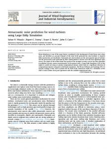
Figure 1.

0

x

−0.6 −0.6 −0.4 −0.2

0

0.2

0.4 z

Typical grid and FWH surface: side view through axis (a), vicinity of the nozzle exit (b), and end view at nozzle exit (c). Lengths normalized with jet diameter.

cylindrical coordinates. A review of some other techniques proposed in the literature to resolve the singularity issue can be found in Constantinescu and Lele [29]. In particular, the singularity can be also eliminated when using a Fourier method in the azimuthal direction, by removing the modes that do not represent a smooth field. However, this is not practical in a general-purpose code, and it seems to address only the immediate vicinity of the axis. Another solution is an unstructured grid, but this is not the option taken here, high-order low-dissipation numerics being extremely challenging to implement on such grids. The end view in Fig. 1c demonstrates good control of the grid density thanks to the two blocks, without waste near the axis but with a fine axisymmetric distribution where the thin shear layer is located. Fully Cartesian or fully cylindrical topologies are much less efficient. On the other hand, the second-order interpolation used to transmit the flow parameters at the block interface and the inevitable loss of accuracy at nodes next to the boundary, where centered second-order differences are used, both result in a localized loss of resolution. The same applies at the four corner


2-8-05

4:03 pm

Page 222

222


(a)

(b) ∂p/∂t

10 y

10 y

5

5

0

0

−5

−5

−10

−10 0

Figure 2.

10

20

x

0

10

20

x

Snapshots of pressure time-derivatives (normalized with ρ 0 , c0 , D ) from simulations of M = 0.9 isothermal jet on grids with expansion rate of the x-spacing 1.013 (a) and 1.04 (b).

“singularities” that stretch a total angle of 270° to 360°. However, these drawbacks are not severe, and have no visible effect on the solutions. The grid is stretched both in x – and r – directions, with rather large grid steps near the free boundaries. As seen in the figure, the full LES domain is much larger than the FWH domain, which is viewed as the useful domain. The FWH domain extends to about 25 diameters streamwise, but the full domain including the buffer layer (see below) extends to 50 diameters. This provides natural damping of the fluctuations in this area and weakens wave reflections at the boundaries. On the other hand, it is very important to stretch the grid in the streamwise direction very gradually inside the turbulent region; otherwise stretching causes false sound generation due to grid-induced deformation of the vortices. This is illustrated in Fig. 2, where we compare snapshots of the pressure time derivative (with levels in the acoustic range, as opposed to the turbulence range) from two simulations of the M = 0.9 jet. One is on a grid with stretching coefficient in x – direction equal to 1.013 in the range 10 < x / D < 31 (this grid is shown in Fig. 1) and the other is on a similar grid but with stretching coefficient of 1.04. The latter reveals a spurious source of sound at x ≈ 14D, identified by a family of relatively weak near-concentric waves propagating from this location. 3.1.2. Boundary conditions and near-boundary treatment The design of non-reflective inflow/outflow boundary conditions and other tools for suppressing reflections from the boundaries (e.g., sponge-like layers of different kinds) is a challenging CFD/CAA issue. Another challenge, especially important for jet noise, is the formulation of physically correct inlet conditions that provide a realistic flow behavior in the jet entry region. In the present work, the following set of boundary conditions and near-boundary treatment has been implemented. At the nozzle exit and at the left boundary of the domain outside the nozzle, we impose profiles of the streamwise velocity and temperature, and set the tangential velocity to zero. To set the pressure, we use the one-dimensional non-reflecting boundary


2-8-05

4:03 pm

Page 223


223

condition proposed by Engquist and Majda [30] ∂p / ∂t + (u − c)∂p / ∂x = 0 for subsonic inlets, and a prescribed pressure value for supersonic inlets. Considering our final goal (noise prediction for the high-Reynolds-number jets from real airliner engines with very thin nozzle boundary layers), the streamwise velocity profile imposed at the nozzle exit is the thinnest one that can be resolved, at least marginally, on affordable grids. As a result, with a typical near-wall grid step in the r-direction of 0.003 D, we set an inflow jet velocity profile with boundary layer thickness 0.035 D and momentum thickness 0.004 D (see Fig.3). In case of non-zero co-flow, its inflow velocity profile has the same shape and width as for the jet. The inflow temperature profiles are uniform, both for the jet and for the co-flowing stream. At the “funnel-shaped” lateral boundary of the LES domain, we use extrapolation of the radial velocity, ur. Its sign defines whether the point is locally an “inlet” or an “outlet” region (the latter happens only in a transient regime, for a large computational domain). Then, if a point is “inlet”, we impose the streamwise velocity, ux , equal to the co-flow velocity and set the azimuthal component, uϕ, to zero. We further assume that the ambient parameters (p0,T0,ρ0) are known, use the “isentropic” relation p/ ρ γ = p0 / ρ 0 γ and the speed of sound defined as c = 0.5(cextr + c0), where cextr is a value obtained by linear extrapolation from the interior grid nodes and c0 is the speed of sound in the ambient air. At the outlet points of the funnel, along with ur, we extrapolate the other two velocity components and the quantity p / ργ, and use the same relation for the speed of sound. At the right (outflow) boundary of the domain, we impose the first-order accurate zero-x – derivative condition for all the variables, including pressure. Although such conditions are mathematically sub-optimal, they still work thanks to holding the pressure at the funnel. Also, these conditions are the only ones we tried that tolerate events of negative streamwise velocity, which are associated with jet turbulence in a zero co-flow.

1

0.8

U/Uj

0.6 0.4

0.2 0

Figure 3.

0

0.02

0.04 0.06 (0.5 - r/D)

0.08

0.1

Normalized velocity profile at the nozzle exit used in the computations.


224

2-8-05

4:03 pm

Page 224


Even without any special measures, other than an appropriate grid coarsening in the near-boundary regions, these boundary conditions do not cause reflections from the boundaries, strong enough to contaminate the solution in the near-field jet area where the FWH surfaces are placed. This was verifed by examining animations of the pressure time-derivative fields (in the acoustic range), and also by comparing the noise predictions obtained with the boundary conditions just described and some with additional “absorbing” layers (see below). In addition, with these boundary conditions the simulations predict a mean entrainment rate close to those obtained in Ref. 7 with elaborate boundary conditions and, also, with those we have obtained in steady RANS calculations of the flow with the use of the vt – 92 turbulence model of Ref. 31 which was specially tuned for axisymmetric compressible jets. Nonetheless, in order to accelerate the transient to a statistically mature solution it is helpful to place an “absorbing” stationary layer along all the boundaries, except for the nozzle exit. The idea originates with Freund [32], and the simple implementation we use in the present work was suggested by Ashcroft and Zhang [33]. It consists in a smooth matching of the evolving and a “target” flowfield within the layer with the use of the relation F(l ) = (1 − s) ⋅ F * (l ) + s ⋅ Ftarget (l ). Here F* is the “calculated” flow quantity (from the solution on the current time step) at the considered point, Ftarget is the corresponding target quantity at the same point, s = (l / L)β, L is the width of the layer, and l is the distance from the internal boundary of the layer to the considered point (0 < l < L). The specific target solution we use is a steady vt –92 RANS solution, and the values of the control parameters are adjusted in the course of preliminary simulations as follows: β = 3 (as in Ref. 33); L = (15 – 20)D at the outflow boundary, 5D at the funnel, and 3D at the left boundary. These values, roughly proportional to the extension of the computational domain in the corresponding directions, achieve the absorption of the waves without any noticeable reflections. They derive from a series of tests. With narrower buffer layers, reflections become visible, although still very slight. Conversely, wider layers can corrupt the “flow visualization” or even the noise-generating regions. In addition to the use of the absorbing layer, in order to speed up damping of the disturbances in the near-boundary region, within the absorbing layer, the order of the upwind part of the scheme is changed from fifth to third. Identifying the overall order of accuracy of the method is far from simple, since the order of accuracy of the many formulas used ranges from first to fifth. Formally, since the lowest order for differencing within the domain is second (for viscous terms) and the lowest order for a boundary condition is first (at the outflow), the answer is that the method is second-order accurate. The time integration is also second-order accurate, and since the practice is to scale the time step proportionally to the grid spacing, the spatial and temporal errors would remain in balance as the grid and time step are refined. The absorbing layers add a difficulty, since they represent a violation of the equation that is fixed (the level of S should, probably, scale with the time step, but the time-step variations have been too narrow for this to be an issue). Reducing the


2-8-05

4:03 pm

Page 225


225

impact of the far-field boundary conditions and absorbing layers is a matter of enlarging the domain; the rate at which errors are reduced by such an enlargement would be estimated from the decay of the solution, which is different in the jet region and in the acoustic region. These estimates have not been made, to our knowledge, and would also require a precise knowledge of the reflection phenomena. When the SGS model is activated, the eddy viscosity can be viewed as an error, which scales with a power of the grid spacing; in principle, the power 4/3 (as was verified in homogeneous turbulence). Therefore, the SGS error could become the dominant one, at least formally. It is in the nature of LES and how the eddy viscosity has been set in classical works that differencing errors are tolerated in order to reduce the SGS error. Essentially, we think of the eddies “missing” because of the truncation, at least as much as we think of the differencing errors. The less formal answer is that the errors due to far-field treatments (numerical boundary conditions and absorbing layers) are believed to have been reduced to negligible levels, based on visualizations specifically aimed at revealing those errors. The crucial region, essentially the one contained inside the FWH surface, enjoys differencing of at least fourth order for the convective terms, which dominate over the viscous terms, so that the second–order differencing of the latter is irrelevant (SGS terms being inactive in this study). Time integration is second-order accurate, so that temporal errors would dominate in the fine-grid limit. Concretely, the effect of grid refinement on the initial shear-layer instability is powerful, at least with the very thin inflow shear layers used here, and this would influence the global solution through receptivity and instability mechanisms, which are again quite complex and nonlinear. A demonstration of the order of accuracy of the code is possible in a simple non-turbulent flow with straightforward boundary conditions, but would not be highly relevant to the much more involved situations of interest here.

3.1.3. Results supporting the strategic choices for CFD With regard to LES, our primary “strategic” choices include not using any inflow jet forcing (steady velocity profile at the nozzle exit), the de-activation of the SGS model, and using a numerical method with a subtle numerical dissipation that is compatible with the spirit of LES (away from walls). Figure 4 visually displays what these choices result in, and what would be observed with alternate approaches. It presents vorticity snapshots from four simulations of M = 0.9 isothermal jet at ReD = 104. The first was performed with the chosen technique; the second with an active LES model (a subgrid version of the Spalart-Allmaras [34] turbulence model (SA SGS model) proposed and calibrated in Refs. 35, 36); the third and fourth without SGS model but with upwind schemes, fifth- and third-order accurate respectively (zero weight of the centered scheme). The grid used in all the simulations is the same, with around 500,000 nodes total, and inner and outer blocks of 151×13×13 and 171×52×50 size. Fig. 4a shows that in spite of the absence of unsteady perturbations at the inflow, the current approach results in a plausible representation of all the features typical of the initial region of high-Reynolds number jets (fast shear-layer roll-up, three-dimensionalization, and


2-8-05

4:03 pm

Page 226

226


(c)

(a) y 1

y 1

Standard case: Hybrid 5th/4th

0

0

−1

−1

0 ω

0.50

2 0.81

1.32

4 2.15

6 3.49

5.68

8 9.23

x

0

2

4

6

8

x

2

4

6

8

x

15.00

(b) y 1

5th order upwind

(d) y 1

LES (SA SGS model)

0

0

−1

−1

0

Figure 4.

2

4

6

8

x

3rd order upwind

0

Snapshots of vorticity magnitude from simulations: with standard approach (a); with SGS model (b); and with upwind-biased schemes applied over the entire domain (c, d).

transition to turbulence), a realistic shape for the jet potential core, and well defined turbulent structures in the developed jet region. Other LES strategies are visibly less successful. If the same (hybrid) numerics are used, but the SGS model is activated, the transition to turbulence is crucially delayed (by many diameters, Fig. 4b). Similarly, if the SGS model is de-activated but fullyupwind schemes are used, the delay is even more pronounced due to more dissipative numerics (Fig. 4c, d). In the initial region of the jet, the simulations with upwind schemes display large, relatively smooth and almost axisymmetric vortices, which consistently yield a large overestimation of the jet noise (by up to 6dB), especially in the lateral direction. A highly plausible explanation is that an event such as roll-up or pairing that is in phase over a significant azimuthal range constitutes a stronger source of sound than un-correlated, narrow similar events. Also, the attribution of the lateral sound to the shear-layer events is well established. Inflow forcing with adequate temporal and azimuthal dependence is a possible remedy to this problem, but at the expense of introducing a number of arbitrary parameters, as already mentioned. These visual observations begin to build credibility in the CFD tool developed here. Additional evidence is given in Section 4, based on a grid-refinement study. On the other hand, we recognize that full-size flows should have “LES content” (i.e., resolved eddies) in the incoming boundary layers; however, the compromises between feasibility and realism will be difficult. Injecting perturbations at the inflow that are physically justified and free of arbitrary adjustable parameters may still be the key to a transition process that is fully credible, since the turbulence would obey boundary-layer physics, and more reproducible, especially if it were able to remedy the transition delay in Figs. 4b-d.


2-8-05

4:03 pm

Page 227


227

3.2. Calculation of far-field sound For some aeronautical applications such as cabin noise and skin fatigue, the pressure is needed a few diameters from the jet, and can be produced directly by the LES. However, in many applications, the far-field sound is the focus, and it would be very un-economical to extend the fine-grid region of the LES far enough to secure far-field behavior and allow extrapolation to large distances. This leads to calculating the far-field sound using information only from the high-quality region of the LES, and considering the outer region of the LES grid as a “cushion” that relegates the inexact boundary conditions or buffer zones far enough from the turbulence, but does not support the sound waves accurately. This subsection gives the details of the formula and discusses a number of issues and modifications made to deal with the realities of numerical simulations and with the infinite extent of the turbulent region, particularly for the more complex jets, while obtaining the highest possible accuracy. 3.2.1. Basic FWH formula We start from equation (14.87) in Dowling [22]. It is a version of the FWH formula for a moving, permeable surface. The observer is stationary at x in the atmosphere, its time is denoted by t, and the FWH surface ∑ is translating at a velocity U. The Mach number in the direction of the observer is Mr = U ⋅ x /(c |x|) . This is a far-field formula: |x| is large compared with the length of the turbulent region. The next term is of higher order in 1/|x|. As already mentioned, the use of the far-field formula removes the possibility of checking the consistency between the sound directly extracted from the LES and that calculated from the integral formula. However, this formula is noticeably simpler, which boosts the efficiency of the code. The formula gives the pressure fluctuation p′ as the sum of “quadrupole”, “dipole” and “monopole” terms: 4π 1 − Mr x p ′( x, t ) = +

∂ x c02 ∂t xj

∫ [ p ′n Σ

j

x j xk ∂2 x 2 c02 ∂t 2

∫ [T ] dV jk

V

]

+ ρu j (un − Un ) d Σ +

∂ ∂t

∫ [ρ u

0 n

Σ

]

+ ρ ′(un − Un ) d Σ

(2)

Here c0 is the far-field speed of sound, Tjk the Lighthill tensor, and n the outward normal vector on ∑; un is u . n. Square brackets denote a quantity taken at the retarded time τ, which satisfies τ = t − |x − y − Uτ |/ c0 , and y is a coordinate with respect to an origin that moves with ∑. With |x| in the far field, τ is approximated by (1 − Mr )τ = t − |x|/ c0 + y j x j /(|x| c0 ) . This is used to convert derivatives from t to τ : ∂τ = (1− Mr)∂t for fixed x and y. The factor |1 − Mr | was taken out of the integral, because ∑ is rigid and non-rotating. Much interest resides in spectra, and Fourier transforms greatly simplify the application of retarded times, which amount to a phase shift by −ω y j x j /[(1 − Mr ) |x| c0 ] where ω = 2πf and f is the frequency in the source coordinates (y,τ). We defer the issue of the


2-8-05

4:03 pm

Page 228

228


ends of the time sample to Section 3.2.2. The transforms are denoted by a hat when the symbol fits, and FT when it does not. A factor e iω x / c0 , which is a uniform phase shift, is dropped. We arrive at:  ω  4π 1 − Mr x pˆ  x,  1 − Mr   x j xk

=

1 x 2 c02 1 − Mr

+

xj

+

x c0

∫ Σ

V

 ∂[ p ′n j + ρu j (un − Un )]  − iω y j x j [(1− Mr ) x c0 ] FT  dΣ e ∂τ  

 ∂[ ρ 0 un + ρ ′(un − Un )]  − iω y j x j [(1− Mr ) x c0 ] dΣ e  ∂τ

∫ FT  Σ

∫

 ∂ 2 Tjk  − iω y j x j [(1− Mr ) x c0 ] FT  dV 2 e  ∂τ 

(3)

The product of the LES therefore consists in the time histories of terms such as ∂[ p ′n j + ρu j (un − Un )]/ ∂τ on a properly-located surface ∑, such that dropping the quadrupole term is acceptable. These time histories are stored in the course of a simulation with a time interval ∆τ over a long enough sample T (200-300 convective time units, D/Uj, in the simulations presented below) and then post-processed in accordance with eqn (3). As a result, we obtain the FT of the acoustic pressure pˆ for different observer directions defined by the azimuthal angle, ϕ, and the angle θ between the jet axis and the radius-vector of the observer. The final result of the acoustic post-processing, i.e., the far-field sound pressure level as a function of the non-dimensional frequency St = fD/Uj and θ, is obtained after averaging of | pˆ |2 over ϕ. 3.2.2. Ends of the time sample, and time derivatives The usual issue with finite samples of a turbulent signal is present, namely, that Fourier series are taken of a signal that is not periodic. This imposes a parasitic component of order 1/f at high frequencies f close to the highest captured frequency fmax = 1/(2∆τ). This parasitic component becomes of order 1 if derivatives are taken in Fourier space using the formula FT(∂ψ /∂τ) = –iωFT (ψ). Then, if the amplitude of the signal “discontinuity” at the ends of a sample is large, as it occurs at the outflow closing disk, it invades the whole spectrum (Ref. 19). For this reason, the τ – derivatives in eqn (3) are produced by the time-differentiation of the LES itself, as opposed to the procedure of storing raw quantities, Fourier-transforming them, and then multiplying by (–iω). This takes more storage, but, in addition to the crucial improvement of the outflow disk treatment described in detail in Ref. 19, has advantages such as improved spectra from relatively short time samples. Windowing the signal would lessen the end problem, but the waste of sample at each end would be significant. In this work, the upper end of the spectrum is discarded, because it is contaminated by insufficient resolution (Ref. 19). Furthermore, the upper frequency limit is arbitrary, in the sense that the FWH


2-8-05

4:03 pm

Page 229


229

integrands are saved only every few LES time steps, typically 5. As a result of the truncation, the spectrum is not steep in the region where it is cut off, and a 1/ f “tail” would hardly be noticeable. Only a DNS would be finely-resolved enough for this to be an issue. In addition, the tail level would depend on the total length T of the time sample roughly as 1/( fT), which would provide an alert when results with different values of T are compared. A separate issue is the shape of the database provided to the FWH integral, in space and time. It is easy to save a database that contains the same source-time interval [τ1, τ2] for all points. However, in order to produce time signals at a reception location x, the source-time interval depends on both x and y. If this is not done, the ends of the signal at x are contaminated, over a duration of up to L/c0, where L is the diameter of the FWH surface (due to the Fourier transform, the procedure effectively “borrows” data from the other end of the interval). This was verified in a few cases by calculating, separately, the Fourier transforms over the exact source-time interval for each y and each direction x j /|x|. After an inverse Fourier transform to the time domain, a clear difference was indeed observed near the ends of the time sample, and only near the ends. However, the effect on spectra was very slight (the time sample being many times larger than L/c0). Therefore, the simpler procedure is used with a single τ interval, which is considerably less costly because the Fourier transforms in eqn (3) are calculated only once. 3.2.3. Limits on the validity of the FWH formula as it is used The exact forms of the Lighthill and FWH formulas demand the solution over the entire space, and are in that sense circular, as explained by Crow [37]. In a numerical context, they are inevitably approximated to make use of a finite amount of information, inside a finite spatial domain and a finite time sample. The most typical approximate step, which is taken here, is to omit the external quadrupoles in the FWH formula, thus reducing the dimension of the integral from four to three and leading to an approach that is not deeply different from a Kirchhoff integral. Then the FWH surface “should” surround the entire turbulent region. This is practical for idealized situations such as a group of vortex rings, but unfortunately not for bluff-body wakes and jets. In these flows, the turbulent region extends to infinity and exhibits a rather slow decay of the fluctuation levels. Ribner [38] estimated that the sound power emitted (in the sense of Lighthill) near the streamwise section of the jet at Y decays very fast, namely as Y–7, strongly supporting the idea of truncating the domain at a low penalty. However, this was derived and is plausible only for a cold static jet. In contrast, for a hot jet with co-flow, the velocity and density differences decay as Y–2/3 instead of Y–1, and the turbulence scale increases as Y1/3 instead of Y for large Y. This scaling is obtained from dimensional analysis, following Cebeci and Bradshaw [39]. For large Y the velocity differences are much smaller than the co-flow velocity, UCF, and the evolution is viewed versus time, Y/UCF, instead of distance, Y, which alters the power laws. In addition, the conserved quantity is the integral in the cross-plane of the velocity difference, instead of the velocity difference squared as in a static jet. This gives the power laws for velocity and length


230

2-8-05

4:03 pm

Page 230


of the dominant eddies. The temperature differences inherited from a hot jet are assumed to follow the same scaling as the velocity; finally, the pressure is assumed to be uniform across the jet, to leading order, so that density differences scale like temperature. Then, an analysis equivalent to Ribner’s leads to the power emitted near Y decaying in proportion to Y−11/3, which is much less favorable than Y–7. This is not a definitive answer, because it strongly depends on the scaling assumed for frequency, which has been controversial. In fact, another plausible scaling for the frequency (using the co-flow velocity instead of the fluctuating velocity) gives Y–1, which is even considerably less favorable. Actually, this latter scaling cannot be correct, since it predicts an infinite energy radiation, which illustrates the limitations of this type of analysis. However, it is a warning against treating complex jets the same as simple jets, in terms of sizing the fine-grid region and the FWH surfaces. New sensitivity tests are in order for each new family of cases, which is done in the applications in Part 2. Derivatives or Ribner’s analysis are not conclusive enough for the general case. The terms that are neglected in the far-field FWH formula are of the order (D/r)/Ma /St compared with the terms that are retained, where r is the observer distance and Ma ≡ Uj /c0 is the jet acoustic Mach number. This order-of-magnitude analysis does not consider possible near-cancellations in integrals. It shows that the far-field approximation is valid as (r/D) → ∞, of course, but not uniformly: it is not as accurate for lower frequencies. Typically, values of St in the simulations extend formally down to 5.10–3, Ma is of order 1, and r/D is of the order of 60 at the least in experiments, so that for the lowest frequencies (up to St ≈ 0.05) the comparison with experiment may be contaminated since the quantity (D/r)/Ma /St is not far below 1. However, the bulk of the sound is produced near St = 0.2 ÷ 0.3 and higher, for which the quantity is well below 0.1, and the focus of the experimental comparisons is in that range. When predictions of aircraft community noise are sought, r/D is far larger than in laboratory experiments, and the far-field formula is very adequate. Conversely, for predictions of cabin noise, the ratio r/D is often below 10, and the pressures will probably be extracted directly from the LES. 3.2.4. Sizing of the FWH surface; “closed” versus “open” surfaces The optimal FWH surface is clearly not the outer boundary of the LES domain, because the waves suffer dispersion and dissipation before reaching that boundary, which in addition imposes imperfect conditions. To minimize losses, the FWH surfaces are fairly tight around the turbulent region, and tapered as seen in Fig.5, where we show a typical set of “nested” surfaces of different width and length together with a snapshot of the magnitude of Lighthill’s source term, a good “indicator” of correctness of a surface placement. Cylindrical shapes of the control surfaces would allow some analytical formulas to be used, but force the upstream part of the sleeve farther from the strongest sound production, especially at high frequencies. Making the FWH surface follow grid surfaces, besides being convenient, gives them a natural shape that skirts the turbulent region, except of course at the end. There, the surface includes a “closing disk” beyond which the neglect of the quadrupole term is obviously a source of error. A basic test of the FWH procedure is that the sound should not be strongly dependent on the surface


2-8-05

4:03 pm

Page 231


231

Σ∂2Tij/∂xi∂xj

y 6 4

40.00

S3

S2

25.24 15.92

2

S1

10.05

L1

0

6.34

L3

L2

4.00

S1

−2

2.52 1.59

−4

1.00

S2

S3

−6

0.63 0.40

0

Figure 5.

5

10

15

20

25

x

30

Typical set of nested FWH surfaces, and snapshot of Lightill’s source term.

used; many comparisons were conducted between nested surfaces, both in terms of diameter and length in Ref. 19, and again here for many of the cases. An example that addresses both the sensitivity of noise predictions to the size of FWH surfaces and the issue of using “closed” versus “open” surfaces is presented in Figs. 6, 7, which show the sound pressure level (SPL) spectra averaged over a frequency interval ∆St = 0.02 in order to make them less “noisy” (Fig. 6) and the overall SPL directivity (Fig. 7) from the basic M = 0.9 jet simulation on the “fine” grid (Fig. 1) obtained with the use of open and closed, “tight” (S1) and “loose” (S3), “short” (L1) and “long” (L3) FWH surfaces of the set depicted in Fig. 5. As far as the closing disk is concerned, Fig. 6 clearly demonstrates a poor behavior of the spectra in the simulations without disks for both tight (frames a, b) and loose (frames c, d) surfaces. However, the deficiency for these two types of surfaces is caused by different reasons. For the tight open surfaces with the sleeve location in the non-linear near-field of the turbulent region, the inaccuracy is caused by the “pseudo-sound” (Refs. 40, 41) generated by the convection of relatively slow vortices in the vicinity of the downstream end of the FWH surface. With the closed surfaces, the pseudo-sound is absent due to the proper cancellation of the “signals” from the sleeve and closing disk (this is revealed by a more detailed analysis of the inputs of different parts of the FWH surface into the total sound signal). As a result, the simulations with open surfaces exhibit a strong unphysical growth of the spectra at low frequencies, the contaminated frequency range becoming wider with the surface length, xend, diminishing (the upper boundary of the range reaches St ≈ 0.15 at xend /D = 17), whereas the closed-surface predictions reveal physically correct decay of SPL at low frequencies. Note that these results are a clear indication that conclusions based on the analysis of Ref. 42 of the errors in sound prediction due to the opening of Kirchhoff (i.e., “linear”) surfaces are not applicable to the tight FWH (“non-linear”) surfaces. Similar experiments for more complex jet flows considered in Part II (ref. 28) show that the contamination of the low-frequency end of the spectrum with tight open surfaces is strongest at low Mach numbers and for cold jets. This is due


2-8-05

4:03 pm

Page 232

232


(a)

(b) θ=90°

100

90

100 1 2 3 4

90

80

80 10−1

100

10−1

St

(c) θ=90°

SPL, dB

90

100

90

80

80 10−1

Figure 6.

100

10−1

St

100

St

Effect of FWH surface on sound spectra (per unit of Strouhal number) for M = 0.9 isothermal jet: “tight” surfaces S1 (a, b); “loose” surfaces S3 (c, d); 1 – open, short (L1) surface, 2 – open, long (L3), 3 – closed, short, 4 – closed, long. Distance 120 diameters.

(a)

(b) 105

OASPL, dB

105

OASPL, dB

St

θ=20°

110

100

100 1 2 3 4 5 6

95

90

100

(d)

110

SPL, dB

θ=20°

110

SPL, dB

SPL, dB

110

0

Figure 7.

20

40

60

80

100 120

θ°

100

95

90

0

20

40

60

80

100 120

θ°

Effect of FWH surface on sound directivity for M = 0.9 isothermal jet: “tight” surfaces S1 (a); “loose” surfaces S3 (b); 1 – 4 as in Fig. 6; 5 – experiment of Lush [43], 6 – experiment of Tanna [44]. Distance 120 diameters.


2-8-05

4:03 pm

Page 233


233

to the relatively slow vorticity decay in such jets, on one hand, and the low overall noise level, on the other hand. For loose open surfaces (Fig. 6,c, d) with the sleeve in the region of much weaker (but still noticeable) non-linearity, the above spectrum deficiency is much less significant and is seen only at St < 0.05. However, as might be expected, another problem shows up at small observer angles: sound is “lost” due to the large “angle of vision” of the surface end (Fig. 6d). This deficiency is absent for the closed FWH surfaces, although, irrespective of being closed or open, the trouble with the loose surfaces is the demand of keeping a fine r – grid up to the sleeve, i.e., far from the turbulent flow region, in order to diminish the dissipation of the sound waves while propagating to the control surface. In the case considered, the latter effect is responsible for a rapid drop of SPL at St > 1 observed with the loose surfaces (compare the high-frequency ends of the spectra in frames a and b versus those in frames c and d of Fig. 6). Consistently with the spectrum behavior, the OASPL predictions with the tight open FWH surfaces, at least when integrated without discarding the low-frequency end, turn out overestimated especially at large observer angles, where the discrepancy with experiment reaches the level of 5-6 dB (Fig. 7a). Conversely, loose open surfaces lead to a significant under-estimation of the OASPL for θ < 40°, i.e., at the peak radiation directions (Fig. 7b). The OASPL obtained with all the considered closed surfaces agrees with experiment much better (putting it within 2-3 dB “target” accuracy), although a 5°-10° shift of the directivity maximum towards larger angles is clearly seen. An important practical outcome of the presented results is also the fact that, with the closed control surfaces, there is no need for arbitrary truncation of the low-frequency range in the OASPL integration. This is different from many studies (see, e.g., Refs. 7, 11, 16), in which unphysical growth of the spectrum at low frequencies, similar to that observed here for the tight open surfaces, forced the authors to discard the frequencies St < 0.05 and even St < 0.15. As for the FWH-surface sensitivity of the noise prediction, for the open surfaces, due to the reasons outlined above, it appears rather significant (at least, if tight and/or relatively short surfaces are used). For the closed surfaces it is much weaker in terms of the SPL spectra and is almost negligible for the OASPL directivity, unless the surface is so short that it does not enclose the major sound sources. Judging from the OASPL curves in Fig. 7, the length of the shortest of the considered surfaces L1 (xend = 17 D), is close to the lower limit of “valid” surface lengths for the static jet: an indication of too short a surface is a small rise of the OASPL at the smallest and largest observer angles compared with the long surfaces L3. It is absent when the “mid-long” surfaces L2 (not shown in Fig. 7) of length xend = 21D are used to compute the noise. Therefore, the error caused by neglecting the quadrupole term downstream of the closing disk becomes “small enough” at this distance from the nozzle. Of course, jets in a co-flowing stream require tangibly longer FWH surfaces and computational domains. As mentioned in the Introduction, our conclusions about the preferability of closed versus open surfaces are in strong contradiction with Ref. 16 (in which closing the surface led to some improvement of the OASPL predictions for 25° < θ < 40°, but also caused a strong unphysical growth at θ > 60°) and Ref. 15 (in which a contamination


2-8-05

4:03 pm

Page 234

234


of the OASPL was observed for any reasonably short control surface, if it was closed). Unfortunately, it is difficult to establish the reason(s) of the contradiction, in particular without knowing details of the FWH approach implementation used in the studies of Refs. 15,16. 2

3.2.5. Substitution of p′/c 0 for p′ This and the following subsection present further steps taken to alleviate the outflowdisk errors. Omitting the quadrupoles in the FWH equation implies assuming that the FWH surface is outside the turbulent region. Therefore, it is consistent to assume that the flow is isentropic on the surface. In that case, substituting p ′ / c02 for ρ′, or more generally ρ0 (p/p0)1/γ for ρ, in eqns (2), (3) is a neutral step. It was verified in the simulations that this isentropic (ρ-p) relation is accurately satisfied on the sleeve, which constitutes the fully-valid part of the FWH surface. The substitution has essentially no effect on the sleeve’s contribution to the sound. The interest is at the outflow disk. In that region, pressure fluctuations are much milder than density fluctuations are for hot jets (by more than an order of magnitude). Therefore, the substitution considerably weakens the parasitic contributions to the sound (pseudo-sound). This effect is significant for static hot jets, and becomes crucial for hot jets with co-flow. This is seen in Fig. 8, which compares the OASPL directivity for a jet with co-flowing velocity UCF/Uj = 0.208 and temperature Tj / T0 = 2.66 with experimental data of Ahuja, Tanna, and Tester [45]. The substitution improves the noise predictions by over 10 dB.

UJ /c0=1.25, TJ / T0 = 2.66, UCF / UJ = 0.208

OASPL, dB

110

105

100

95

0

Figure 8.

20

40

60

80

100

120

140

θ°e

Effect of ρ ′ − p ′ substitution on sound directivity for hot jet with co-flow: solid line – with the substitution; dashed line – without. Experiments from Ahuja, Tanna, and Tester [45]. Distance 100 diameters.


2-8-05

4:03 pm

Page 235


235

This substitution does not amount to the assumption that the turbulent plume crossing the disk is isentropic; it is simply a version of the equation that is much less vulnerable to entropy fluctuations than the standard equation. A very similar step would be to apply the Kirchhoff equation to pressure, instead of density. This approach appears to be a better option than discarding the contribution of the disk (using an “open” surface), for the reasons discussed in the previous section. An additional reason is that it preserves the correct contribution of the outer region of that disk, which is in isentropic flow. In earlier work, an arbitrary “hole” was cut out of the disk, giving a partially open surface. For cold jets, the effect of the ( ρ′ − p′) substitution is either negligible (for FWH surfaces of “valid” length, e.g., xend > 20 D for static jets), or small but positive (for shorter surfaces). Therefore, it is always used. 3.2.6. Averaging over outflow disks This step is also taken to extract the sound more accurately even though some assumptions are violated at the outflow disk, but its effect is not as strong as that of the ( ρ′ − p′) substitution. Its effect is noticeable only for jets with co-flow, which are characterized by a slow decay of vorticity and almost uniform convection of relatively weak vortices in the streamwise direction at large distances from the nozzle. Also, in contrast to the (ρ′ − p′) substitution, it is more significant for the cold/isothermal than for the hot jets, because of faster decay of vorticity in the latter. The premise is that the FWH convolution integral “selects” wave components that are propagating towards the observer at the speed of sound (and therefore have at least a sonic phase-velocity magnitude); see equations in Section 3.2.1, and recall the arguments in support of Mach waves in the literature. This selection is effective if the − iω y j x j /(|x|c0 ) phase of the oscillating function e has a sufficient variation (several cycles) over the surface of integration. It fails if the surface is severely truncated and for the outflow disk, which is small, especially for observer directions close to the jet axis (xjyj varies very little). This leads to the idea of averaging the sound calculated from two or more FWH surfaces of different lengths at the outflow, in the same LES. Note that the complex Fourier transforms of the signals from each surface are averaged, not their magnitudes, since the phase is key; this is equivalent to averaging the raw time signals. The parasitic, non-acoustic fluctuations translate at lower velocities than the sound, certainly for the Mach numbers that prevail near the outflow disk, and therefore are cancelled to some extent by the averaging, provided the distance between the disks is not small compared with c/ω. Closing the FWH surface with a cone instead of a disk would probably have a similar effect. The effect of this averaging is illustrated by Fig. 9, where we present results of the noise calculation for the M = 0.9 isothermal jet in a co-flowing flow with velocity UCF /Uj = 0.3. The averaging was performed over up to six disks, with a total distance between them of 10 diameters, from x/D = 30 to x/D = 40. As seen in the figure, the effect can reach up to 4 dB in the forward quadrant, at angles such as 150° from the jet axis. This is the direction that maximizes the difference between the phase velocity of the eddies and that of the sound. The effect is almost not noticed near 90°, plausibly because sound in that direction is insensitive to averaging from different x values, and


2-8-05

4:03 pm

Page 236

236


MJ = 0.9, TJ / T0 = 1,UCF / UJ = 0.3

OASPL, dB

90 XEND/= 30 32 34

85

36 38 40 all 6 averaged

80 0

Figure 9.

20

40

60

80

100

120

140

θ°e

Effect of disk averaging on sound directivity for jet with co-flow. Distance 120 diameters.

also because the dipole contribution is nearly zero for the disk in this observer direction. It is not noticed in the downstream quadrant either, this time because the true noise is much stronger in that direction. Disk averaging increases the cost of the sound calculation, but only slightly (noise from a set of nesting FWH surfaces is computed anyway for a routine analysis of its surface-sensitivity), and in fact, its cost could well be offset by allowing a shorter domain. It is therefore routinely used. 3.2.7. Reference frames The sound calculated for an observer stationary in the atmosphere is easily converted to an observer moving with the device, using the radiation condition which is simple in the far-field. The frequency is multiplied by (1 − Mr ) , and the spectral density divided by (1 − Mr ) . The angle is also corrected in the presentation of the results to reflect the position of the nozzle at the time the sound is received. Further corrections, needed to compare with measurements made outside the co-flow in some wind tunnels, must refer to the original papers. 4. GRID REFINEMENT FOR THE “BASIC” M=0.9 ISOTHERMAL JET In any CFD activity, and especially one that attempts to capture as much of the turbulence as is possible on a given grid, the grid dependence of the solutions needs a detailed examination, both through visualizations and in the noise results. In this section, we present results of such a study for the “basic” case of a M = 0.9 isothermal jet at Re = 10 4 .


2-8-05

4:03 pm

Page 237


237

The coarse-grid simulation of this case was carried out in Ref. 19 and is repeated here, now with the use of the ( ρ′ − p′) substitution, although it showed negligible effect in this case. The coarse grid described in Section 3.1.3 has around 500,000 nodes total. The fine grid, with around 1,200,000 nodes total, is that shown in Fig. 1, with the inner and outer blocks of 217 × 17 × 17 and 241 × 70 × 66 nodes. The average grid spacing is down by 25% in the finer grid, and the time step drops from 0.04 to 0.03 convective time units D / U j . Both simulations have aged for near 1000 convective units, which seems sufficient for the establishment of a statistically steady-state up to the downstream end of the FWH surfaces used (the time taken by a particle to travel to x = 25 D on the centerline is about 55 time units, but particles are much slower near the edge of the jet). The last ~250 units of the samples are used for collecting the noise and turbulent statistics. The overall sound intensity is obtained by integration of spectra over frequency intervals 0 < St < 1.0 and 0 < St < 2.5 for the coarse and fine grids, respectively. Comparisons of the results of the two simulations with each other and with experimental data are presented in Figs. 10-15. As far as the effect of the grid on the turbulence is concerned, as seen from the figures, the finer grid delays transition by nearly one diameter (see Fig. 10 with typical snapshots of vorticity and Fig. 11 with spectra of the resolved kinetic energy in the initial region of the shear layer), but the transition “scenario” and the downstream evolution and Reynolds stresses (Figs. 12, 13) remain essentially unchanged. The length xc of the

Figure 10.

Snapshots of vorticity magnitude from simulations of M = 0.9 isothermal jet on coarse (a) and fine (b) grids: 10 levels, from 1.0 to 30.0, with uniform distribution in logarithmic scale.


2-8-05

4:03 pm

Page 238

238


(a)

(b)

10−2

10−2 dk/dSt

10−1

dk/dSt

10−1

x/D = 0.3 1.0 2.0 4.0 −5/3 slope

10−3

x/D = 0.3 1.0 2.0 4.0 −5/3 slope

10−3

10−4 0.1

1

2

10−4 0.1

3

1

St

Figure 11.

(a)

(b) 1/UCL, 5 r05 1/UCL

0.4

3 2

0.2

Figure 12.

5

10

0.10 0.05

1

r05

0

0.15

4 rms(u')

UCL

0.6

0.0

3

Spectra of resolved turbulent kinetic energy in the shear layer at r/D=0.45 obtained on the coarse (a) and fine (b) grids.

UCL 1.0 0.8

2

St

15

20 x

0

0.00 0

1

2

3

x/xc

Effect of grid on streamwise distributions. Mean centerline velocity and its inverse, and jet half-radius (a). Centerline velocity fluctuations (b). Solid lines – fine grid, dashed lines – coarse grid. Experiment of Lau, Morris and Fisher [46] corrected to account for later measurements of Lau [47].

jet potential core (defined as the distance from the nozzle exit to the point where the mean centerline velocity UCL falls down to 0.98U j ) is 4.1D for the coarse grid, and 4.8 D for the fine one. The changes in the transition location and potential-core length are similar to those observed experimentally between nozzles that are identical in diameter, but not in shape. The agreement of both simulations with experiment on mean flow velocity and turbulence of the jet in its fully-developed region is quite satisfactory (Fig. 13), although the peak normal turbulent intensity is up to 20% lower than in experiments. This is not improved by the finer grid, but the refinement was only by a factor 3 / 4 , which in an inertial range recovers only 17% of the missing kinetic energy. In contrast, the shear stress (Fig. 13c) and consequently the spreading rate are very close to experiment. Specifically, the rate of half-radius grows, Ar05 , comes to 0.094 and 0.087, while its experimental value is in the range 0.086-0.096 (Zaman [50]).


2-8-05

4:03 pm

Page 239


239

(a)

(b) 0.3

1

U/UCL

0.8

0.2

0.6

0.15

1 2 3

0.4 0.2 0

0.05

4 5

0

0.05

1 2 3 4 5 6

0.1

0.15 0.1 r/(x–x0)

0

0.2

(c)

0

0.05

0.1 0.15 r/(x–x0)

0.2

(d) 0.3

0.3 (v′v′)1/2/UCL

0.25

0.2

0.15

0.15

0.1

0.1

0.05

0.05 0

0.05

Figure 13.

0.15 0.1 r/(x–x0)

(u′v′)1/2/UCL

0.25

0.2

0

(u'u')1/2/UCL

0.25

0

0.2

0

0.05

0.15 0.1 r/(x–x0)

0.2

Effect of grid on radial profiles of mean axial velocity and Reynolds stresses, normalized with mean centerline velocity and distance to the virtual jet origin. 1 – fine grid, x / D = 15 ; 2 – fine grid, x / D = 30 ; 3 – coarse grid, x / D = 15; 4 – coarse grid x / D = 25; 5 – experiments of Hussein et al [48]; 6 – experiments of Panchapakesan and Lumley [49].

105

OASPL, dB

100

95 Coarse grid Fine grid Expt. (Lush)

90

Expt. (Tanna) 85

0

Figure 14.

20

40

60

80

100

120

140

θ°

Effect of grid on sound directivity. Experiments from Lush [43] and Tanna [44]. Distance 120 diameters.


2-8-05

4:03 pm

Page 240

240


(a)

(b)

120

120 θ =30°

100 90 80

100 90 80

Coarse grid

70 60

70

Fine grid

0

0.5

1

1.5

60

2

(c)

1

0.5

1.5

2

St

1/3-OCT. SPL, dB

100 θ =30°

90 80

70

θ =90°

90 80

70 10−1

Figure 15.

0

(d)

100 1/3-OCT. SPL, dB

θ =90°

110 SPL, dB

SPL, dB

110

100

St

10−1

100

St

Effect of grid on raw (per unit of Strouhal number) and 1/3-octave spectra. Experiments from Tanna [44]. Distance 120 diameters.

The corresponding rates of the centerline velocity decay, Bu , are 6.05 and 6.55 versus 5.4-6.1 and ~7 in experimental studies of Ref. 50 and Ref. 51. Thus on both grids the energy-containing motion is captured, with finer vortical structures displayed on the finer grid, of course. Comparisons of noise predictions on the coarse and fine grids shown in Figs. 14, 15 are also favorable, for the most part. In particular, the difference in the OASPL obtained on the two grids is less than 1 dB for the whole range of observer angles (Fig. 14). The experimental scatter being of the same order, a strong preference cannot be established through such comparisons. The blemish here (not improved by the finer grid) is that the calculated noise peaks roughly 35° from the jet axis, whereas experiments peak closer to 25°. The detailed examination of spectra and of the consistency between LES and FWH in terms of directivity have, unfortunately, not led to any worthwhile conjecture over the cause of this disagreement (which is even more pronounced when using open surfaces, as shown in Section 3.2.4). The refraction of sound by the flow field downstream of the disk was considered, in case it concentrated energy at angles very near the jet axis, but did not seem very significant, nor easy to implement. Work on this issue continues. These results are nevertheless very encouraging, especially at such a low level of computing power.


2-8-05

4:03 pm

Page 241


241

The “raw” and one-third-octave SPL spectra (Fig. 15) are more informative in terms of the predicted sound grid-sensitivity. The coarse-grid spectrum has a peak at a Strouhal number near 1.6, which is spurious, and attributed to vortices in the flow upstream of transition that are almost axisymmetric; strong disturbances of the flow parameters at this frequency in the close vicinity of the nozzle lip are seen clearly in the kinetic energy spectrum in the shear layer at x/D = 0.3 shown in Fig. 11a. The rise for higher frequencies at θ = 90 o also is spurious, judging from its absence with the fine grid. The fine-grid spectrum has a weaker peak, near St = 2.2 , and continues its descent up to St = 2.5 , at least. The agreement of the predicted noise spectra with experiment is close to the target accuracy of 2-3 dB within the addressed frequency range, and improves on the finer grid. Analysis of the spectra obtained on the two grids, together with their surface-sensitivity (see Ref. 19 and Section 3.2.3) gives a good estimate of the reliable range in the spectrum, which is up to around St = 1.5 on the fine grid, at least for the direction close to the peak sound radiation ( θ ≈ 30 o ). Unfortunately, for the fan flow of the largest engines, with a plume diameter near 2.4 m and sonic velocity, this is only about 500 Hz, when the sound needs to be known up to several kHz. Note also that even on the fine grid, the overall sound level at the direction normal to the jet axis benefits from canceling errors between an excess of the order of 3 dB in the region near St = 0.3 ÷ 0.4 , and a deficit beyond St ≈ 1. This probably is an indication of the fact that the simulation still returns excessively large vortical structures at the initial stage of shear-layer roll-up and three-dimensionalization since, as is commonly accepted, exactly this region of the turbulent jet flow is responsible for the high-frequency noise radiated at these observer angles. In general, we can conclude that the results of the grid-refinement study presented above are encouraging and lend credibility to the approach, the more so since similar grid-sensitivity analysis performed for almost all of the many more complex jets considered in Part II [28] yielded close results. However, the drop of the grid spacing in the simulations performed so far can only be described as marginal: a factor near 3/4. On the premise that with the strategy adopted here to make the best use of the resolution, the grid and numerics have some control over the details of transition, which in turn are important at least for the high frequency part of the noise, a further and more aggressive (especially in the initial flow region) grid refinement is desirable. Such simulations are in progress, with a parallelized version of the code. 5. CONCLUSIONS The detail given in this Part I should allow readers to fully identify the ingredients of the method used, and critique them. It should also clarify the meaning of the findings in Part II [28], which covers a number of non-trivial physical effects such as large temperature differences and shock waves, and is quite encouraging. The strategic choices made both for the LES and for the far-field-sound “post-processing” appear vindicated (however, the disablement the SGS model will be reversed at some point, when grids permit it). In particular, the multi-block grid structure is very helpful in offsetting the limitations of the computers used, which confine the grids to less than 2 million points. The search for perfection in simple cases will continue, of course, with one focus on the


242

2-8-05

4:03 pm

Page 242


overall sound levels in directions near the jet axis, and another on the spectrum at right angles to the axis. It is unclear which is more likely to cause each inaccuracy, between the LES and the sound calculation, and detail modifications of each method are frequently tested. Further grid refinement is also in progress, as is research towards a physically sound inflow-forcing concept. In general, although the limitation on resolved frequencies must never be forgotten in the real-life context, the idea that Large-Eddy Simulation will be the method of choice for noise prediction is strongly supported by this study. ACKNOWLEDGEMENTS We are grateful for the many constructive comments of an anonymous referee. This work was primarily funded by Boeing Commercial Airplanes, and partially by General Electric Aircraft Engines, under the supervision of Dr. P. Gliebe. The authors are grateful to Dr. A. Travin, who has adapted the NTS code to jet-noise simulations. REFERENCES [1] Freund, J.B., Noise Sources in a Low-Reynolds-Number Turbulent Jet at Mach 0.9, Journal of Fluid Mechanics, 2001, 438, 277-305. [2] Gamet, L. and Estivalezes, J. L., Application of Large-Eddy Simulations and Kirchhoff Method to Jet Noise Prediction, AIAA Journal, 1998, 36(12), 2170-2178. [3] Shih, S.H., Hixon, D.R., Mankbadi, R.R., and Povinelly, L.A., Large-Scale Simulation of Supersonic Jet Noise, AIAA Paper, 1998, AIAA-98-3014. [4] Choi, D., Barber, T.J., Chiappetta, L.M., and Nishimura, M., Large Eddy Sumulation of High-Reynolds Number Jet Flows, AIAA Paper, 1999, AIAA-99-0230. [5] Zhao, W., Frankel, S.H., and Mongeau, L., Large Eddy Simulations of Sound Radiation from Subsonic Turbulent Jets, AIAA Journal, 2001, 39(8), 1469-1477. [6] Morris, P.J., Long, L.N., Scheidegger, T.E., and Boluriaan, S., Simulations of Supersonic Jet Noise, International Journal of Aeroacoustics, 2002, 1(1), 17-42 [7] Bogey, C., Bailly, C., and Juve, D., Noise Investigation of a High Subsonic, Moderate Reynolds Number Jet Using a Compressible Large Eddy Simulation, Theoret. and Comput. Fluid Dynamics, 2003, 16, 273-297. [8] Bogey, C., and Bailly, C., LES of a High Reynolds, High Subsonic Jet: Effects of the Inflow Conditions on Flow and Noise, AIAA Paper, 2003, AIAA-2003-3170. [9] Bogey, C., and Bailly, C., LES of a High Reynolds, High Subsonic Jet: Effects of the Subgrid Modelling on Flow and Noise, AIAA Paper, 2003, AIAA-2003-3557. [10] Bodony, D.J., and Lele, S.K., Large Eddy Simulation of Turbulent Jets and Progress towards a Subgrid Scale Turbulence Model, in: Huttl, T., Wagner, C., and Delfs, J., eds., Proceedings of International Workshop on LES for Acoustics, DGLR-Report 2002-03, Goettingen, 2002. [11] Andersson, N., Eriksson, L.-E., and Davidson, L., Large-Eddy Simulation of a Mach 0.75 Jet, AIAA Paper, 2003, AIAA-2003-3312.


2-8-05

4:03 pm

Page 243


243

[12] Loh, C.Y., Himansu, A., and Hultgren, L.S., A 3-D CE/SE Navier-Stokes Solver With Unstructured Hexahedral Grid for Computation of Near Field Jet Screech Noise, AIAA Paper, 2003, AIAA-2003-3207. [13] Lupoglazoff, N., Biancherin, A., Vuillot, F., and Rahier, G., Comprehensive 3D Unsteady Simulations of Subsonic and Supersonic Hot Jet Flow-Fields. Part 1: Aerodynamic Analysis, AIAA Paper, 2002, AIAA-2002-2599. [14] Biancherin, A., Lupoglazoff, N., Rahier, G., and Vuillot, F., Comprehensive 3D Unsteady Simulations of Subsonic and Supersonic Hot Jet Flow-Fields. Part 2: Acoustic Analysis, AIAA Paper, 2002, AIAA-2002-2600. [15] Rahier, G., Prieur, J., Vuillot, F., Lupoglazoff, N., and Biancherin, A., Investigation of Integral Surface Formulations of Hot Jets Starting from Unsteady Aerodynamic Simulations, AIAA Paper, 2003, AIAA-2003-3164. [16] Uzun, A., Lyrintzis, A.S., and Blaisdell, G.A., Coupling of Integral Acoustics Methods with LES for Jet Noise Prediction, International Journal of Aeroacoustics, 2004, 3(4), 297-346. [17] Lew, P., Uzun, A., Blaisdell, G.A., and Lyrintzis, A.S., Effects of Inflow Forcing on Jet Noise Using Large Eddy Simulation, AIAA Paper, 2004, AIAA-2004-0516. [18] Shur, M.L., Spalart, P.R., Strelets, M.Kh., and Travin, A.K., Towards the Prediction of Noise from Jet Engines, in: Rodi, W., Fueyo, N., eds., Engineering Turbulence Modelling and Experiments 5: Proceedings of the 5th International Symposium on Engineering Turbulence Modelling and Measurements, Elsevier Science Publishers, Amsterdam, 2002, 699-708. [19] Shur, M.L., Spalart, P.R., Strelets, M.Kh., and Travin, A.K., Towards the Prediction of Noise from Jet Engines, International Journal of Heat and Fluid Flow, 2003, 24(4), 551-561. [20] Spalart, P.R., Strategies for Turbulence Modelling and Simulations, International Journal of Heat and Fluid Flow, 2000, 21, 252-263. [21] Ffowcs Williams, J.E., and Hawkings, D.L., Sound Generated by Turbulence and Surfaces in Unsteady Motion, Philosophical Transactions of the Royal Society, 1969, A264 (1151), 321-342. [22] Dowling, A.P., Effects of Motion on Acoustic Sources, in: Grighton, D.G. et al., Modern Methods in Analytical Acoustics: Lecture Notes, Springer-Verlag, London, 1992, 406-426. [23] Brentner, K.S, and Farassat, F., Analytical Comparison of the Acoustic Analogy and Kirchhoff Formulation for Moving Surfaces, AIAA Journal, 1998, 36 (8), 1379-1386. [24] Strelets, M.Kh., Detached Eddy Simulation of Massively Separated Flows, AIAA Paper, 2001, AIAA-2001-0879. [25] Roe, P.L., Approximate Rieman Solvers, Parameter Vectors and Difference Schemes, Journal of Computational Physics, 1981, 46, 357-378. [26] Van Leer, B., Towards the Ultimate Conservative Difference Schemes. V. A Second Order Sequel to Godunov’s Method, Journal of Computational Physics, 1979, 32, 101-136.


244

2-8-05

4:03 pm

Page 244


[27] Van Albada, G.D., Van Leer, B., and Roberts, W.W., A Comparative Study of Computational Methods in Cosmic Gas Dynamics, Astron. Astrophysics, 1982, 108, 76-84. [28] Shur, M.L., Strelets, M.Kh., and Spalart, P.R., Noise Prediction for Increasingly Complex Jets. Part II: Applications, International Journal of Aeroacoustics, 2005, 4(3&4), 247-266. [29] Constantinescu, G.S., and Lele, S.K., A Highly Accurate Technique for the Treatment of Flow Equations at the Polar Axis in Cylindrical Coordinates Using Series Expansions, Journal of Computational Physics, 2002, 183, 165-186. [30] Engquist, B., and Majda, A., Absorbing Boundary Conditions for the Numerical Simulations of Waves, Mathematics of Computation, 1977, 31, 629-651. [31] Gulyaev, A.N., Kozlov, V.E., and Secundov, A.N., A Universal One-Equation Model for Turbulent Viscosity, Fluid Dynamics, 1993, 28 (4), 484-494 (translated from Russian, Consultants Bureau, New York). [32] Freund, J.B., Proposed Inflow/Outflow Boundary Conditions for Direct Computation of Aerodynamic Sound, AIAA Journal, 1997, 35, 740-742. [33] Ashcroft, G., and Zhang, X.,A Computational Investigation of the Noise Radiated by Flow-Induced Cavity Oscillations, AIAA Paper, 2001, AIAA-2001-0512. [34] Spalart, P.R., and Allmaras, S.R., A One-Equation Turbulence Model for Aerodynamic Flows, La Recherche Aerospatiale, 1994, 1, 5-21. [35] Spalart, P.R., Jou, W.-H., Strelets, M., and Allmaras, S.R., Comments on the Feasibility of LES for Wings, and on a Hybrid RANS/LES Approach, in: Liu, C., Liu, Z., eds., Advances in DNS/LES: Proceedings of the 1st AFOSR International Conference on DNS/LES, Greyden Press, Columbus, 1997. [36] Shur, M.L., Spalart, P.R., Strelets, M.Kh., and Travin, A.K., Detached-Eddy Simulation of an Airfoil at High Angle of Attack, in: Rodi, W., Laurence, D., eds., Engineering Turbulence Modelling and Experiments 4: Proceedings of the 4th International Symposium on Engineering Turbulence Modelling and Measurements, Elsevier Science Publishers, Amsterdam, 1999, 669-678. [37] Crow, S.C., Aerodynamic Sound Emission as a Singular Perturbation Problem, Studies in Applied Mathematics, 1970, XLIX (1), 21-44. [38] Ribner, H.S., Strength Distribution of Noise Sources Along a Jet, Journal of Acoustic Society of America, 1958, 30, 876-877. [39] Cebeci, T., and Bradshaw, P., Momentum transfer in boundary layers, McGrawHill, 1977. [40] Blokhintsev, D.I., Acoustics of a Nonhomogeneous Moving Medium, Nauka, Moscow, 1946 (In Russian. English translation: NACA T.M. No.13). [41] Ffowcs Williams, J.E., Noise Source Mechanisms, in: Grighton, D.G. et al., Modern Methods in Analytical Acoustics: Lecture Notes, Springer-Verlag, London, 1992, 313-353. [42] Freund, J.B., Lele, S.K., Moin, P., Calculation of the Radiated Sound Field Using an Open Kirchhoff Surface. AIAA Journal, 1996, 34, 909-916.


2-8-05

4:03 pm

Page 245


245

[43] Lush, P.A., Measurements of Subsonic Jet Noise and Comparison with Theory, Journal of Fluid Mechanics, 1971, 46, 477-500. [44] Tanna, H.K., An Experimental Study of Jet Noise. Part I: Turbulent Mixing Noise, Journal of Sound and Vibration, 1977, 50, 405-428. [45] Ahuja, K.K., Tanna, H.K., and Tester, B.J., Effect of Simulated Forward Flight on Jet Noise, Shock Noise and Internal Noise, AIAA Paper, 1979, AIAA-79-0615. [46] Lau, J.C., Morris, P.J., and Fisher, M.J., Measurements in Subsonic and Supersonic Free Jets Using a Laser Velocimeter, Journal of Fluid Mechanics, 1979, 93 (1), 1-27. [47] Lau, J.C., Effect of Exit Mach Number and Temperature on Mean-Flow and Turbulence Characteristics in Round Jets, Journal of Fluid Mechanics, 1981, 105, 193-218. [48] Hussein, H.J., Capp, S.P., and George, S.K., Velocity Measurements in a HighReynolds-Number, Momentum-Conserving, Axisymmetric Turbulent Jet, Journal of Fluid Mechanics, 1994, 258, 31-75. [49] Panchapakesan, N.R., and Lumley, J.L., Turbulence Measurements in Axisymmetric Jets of Air and Helium. Part I: Air Jet, Journal of Fluid Mechanics, 1993, 246, 197-223. [50] Zaman, K.B.M., Asymptotic Spreading Rate of Initially Compressible Jets – Experiment and Analysis, Physics of Fluids, 1998, 10, 2652-2660. [51] Simonich, J.C., Narayanan, S., Barber, T.J., and Nishimura, M., High Subsonic Jet Experiments. Part I: Aeroacoustic Characterization, Noise Reduction and Dimensional Scaling Effects, AIAA Paper, 2000, AIAA-2000-2022.


2-8-05

4:03 pm

Page 246

Noise prediction for increasingly complex jets. Part I

Noise prediction for increasingly complex jets. Part I

Suggest Documents