AIAA 2006-485
44th AIAA Aerospace Sciences Meeting and Exhibit 9 - 12 January 2006, Reno, Nevada
Further Steps in LES-Based Noise Prediction for Complex Jets Michael L. Shur* “New Technologies and Services” (NTS), St.-Petersburg 197198, Russia Philippe R. Spalart† Boeing Commercial Airplanes, Seattle, WA 98124, USA Michael Kh. Strelets‡ “New Technologies and Services” (NTS), St.-Petersburg 197198, Russia and Andrey V. Garbaruk§ St.-Petersburg State Polytechnic University, St.-Petersburg 195220, Russia The paper presents the status of a CFD/CAA numerical system developed by this team starting in 2001. The aim is to predict the noise from jets of airliner engines with an accuracy of 2-3 dB over a meaningful range of frequencies, while having no empiricism and a general-geometry capability. The first part of the paper outlines the system itself and some results of its testing (a full-length description is given in a recent two-part paper1, 2)), and the second part presents the latest developments and achievements. These include: an accurate algorithm for shock capturing in LES based on local automatic activation of flux-limiters; a two-step RANS-LES approach to complex nozzles; and a set of simulations of cold and heated jets from round and beveled single nozzles, sonic jets with shocks, jets from dual nozzles (co-planar and staggered, in still air and in co-flowing flow), dual nozzles with fanflow deflecting vanes, and chevron nozzles. Although all the simulations were carried out on PC clusters with a maximum of six processors and on rather modest grids (2-4 million nodes), in most cases the system is close to the 2-3 dB target accuracy both in terms of directivity and spectrum, albeit limited in terms of frequency (to a diameter Strouhal number that ranges from 2 to 4 depending on the grid used and flow regime). The overall message of the paper is that available CFD/CAA numerical and physical models, if properly combined, are capable of predicting the noise of rather complex jets with quite affordable computational resources and already today can be helpful in a rapid low-cost analysis of different noise-reduction concepts.
I
I.
Introduction
N engineering practice, the prediction of noise from jet engines is still based on empirical methods and scaling laws such as Lighthill’s or, at most, on steady Reynolds-Averaged-Navier-Stokes computations combined with ad hoc models for noise sources. The empirical basis of the methods and extreme simplifications of the turbulence responsible for noise generation appear to rule them out as a trustworthy tool for the evaluation of new concepts of noise reduction. Such a tool must deal with many non-trivial features, like wide temperature differences, two-stream flows, imperfectly expanded supersonic streams, jets in co-flowing stream (in flight), non-circular
*
Leading Research Scientist,
[email protected], Senior Member AIAA. Technical Fellow, P.O. Box 3707,
[email protected]. ‡ Principal Scientist,
[email protected]. § Associate Professor, Department of Aerodynamics and Thermodynamics,
[email protected]. †
1 of 26 American Institute of Aeronautics and Astronautics Copyright © 2006 by the American Institute of Aeronautics and Astronautics, Inc. All rights reserved.
nozzles, etc., and must be capable of accounting for the subtle effects of design innovations on the turbulent structures responsible for the noise. These considerations, increasing computing power, and advancing algorithms are the factors driving the field towards LES, the only turbulence-resolving approach feasible at high Reynolds numbers. The application of LES to jet-noise prediction is under way in many research groups now (see the references in Ref.1 and the latest publications3-12)). However most of the studies are more “academic” than “industrial” in that they deal with simple round jets (many of codes lacking general-geometry capabilities) and very few of the “complicating factors” mentioned above. This is partly explained by the extreme demands on the numerical system in order to resolve multiple turbulent scales and by the complexity of combining turbulence and far-field acoustics. Boosting the usefulness of the method therefore means eliminating any waste of computing effort. This highlights the importance of a number of decisions needed for LES-based noise computation, both in the turbulence-simulation and the soundextraction approaches. LES brings up options for: the configuration of the computational domain and topology of the grid; the numerical scheme and boundary conditions; the Subgrid-Scale (SGS) model (if any); the approach to obtaining transition to turbulence, etc. For noise extraction, decisions are needed on using direct or integral methods and, for the latter, a Kirchhoff or Ffowcs-Williams/Hawkings (FWH) formulation, the shape and position of control surfaces, their treatment near the downstream end, etc. All these decisions should be assessed not only separately but as an aggregate as well. An analysis of the state of the art1) shows that the range of approaches being explored is wide, and that the CFD/CAA community is still far from a consensus on the most efficient one. This is fairly normal, considering the complexity of the problem. In this paper, an overview is presented of the non-empirical numerical system developed by the authors over the last 5 years with the final goal of predicting the noise of engine jets within 2-3dB accuracy over as wide frequency range as possible. The approach seems to combine sensibly some elements of the techniques used in the literature with some new ones and, based on the results obtained so far, is rather promising and has a chance to become a reliable industrial tool, although many physical and numerical characteristics can yet be improved. The levels of accuracy and geometry completeness reached are, of course, still not sufficient for airliner certification, and will not be for many years, especially as far as the high frequency noise is concerned. However the extrapolation from laboratory experiments to a certification also has its uncertainties, and flow measurements capable of “explaining” the success or failure of a device are essentially impossible, whereas LES provides the entire flow and sound fields. Therefore, the present value of the method lies in helping a more educated, rapid, and low-cost evaluation of noise-reduction devices. The boosted understanding of the flow physics will also, sooner or later, lead to an invention. The rest of the paper is organized as follows. In Section II a brief overview is presented of the numerical system and major previous results. Then, in Section III a detailed presentation is given of the latest methodological developments (Section III.A) and recent applications (Section III.B). Finally the conclusion section summarizes major achievements and outlines still-unresolved problems.
II. Overview of the Numerical System and Key Previous Results A detailed description of the numerical approach is presented in two journal articles1,2), along with a set of tests supporting the key elements of the strategy. Briefly, the salient features of the system and “strategic choices” made in LES and noise computation are as follows. We use the NTS code (Ref.13), which runs on structured multi-block curvilinear grids with implicit 2nd order time integration and dual time stepping. The inviscid differencing is based on the flux-difference splitting scheme of Roe14). It is a weighted average of 4th-order centered and 5th-order upwind-biased schemes (with typical weights 0.75 and 0.25 respectively) in the turbulent region and acoustic near-field, and “pure” upwind-biased outside that region. The outer boundary conditions are non-reflecting; in addition, a buffer layer is implemented near the outflow. For the turbulence simulation, our current choice is to de-activate the SGS model and to rely on the subtle numerical dissipation of the slightly upwind scheme, which is compatible with the spirit of LES away from walls. This choice is dictated mostly by the crucial importance of a realistic representation of the transition to turbulence in the jet shear layers, which should be provided by a CFD approach for purposes of noise prediction. This representation is inevitably approximate, since resolving the fine-scale turbulent structures of the nozzle boundary layers that seed the shear layer and cause its rapid transition in the real high-Re jets is far out of reach. Other LES strategies that were tested turned out visibly less successful. If the SGS model is activated, the transition to turbulence is crucially delayed. If only the upwind-biased (3rd or 5th order) schemes are used, the delay also is very pronounced, due to more dissipative numerics1). Artificial inflow forcing, as employed in many other jet studies, 2 of 26 American Institute of Aeronautics and Astronautics
could resolve this issue to some extent, but was rejected to avoid the creation of parasitic noise and the introduction of a number of arbitrary parameters. For noise prediction, we use the far-field formulation of the permeable Ffowcs-Williams/Hawkings surface integral method without external quadrupoles, which seems to be the best compromise between efficiency and accuracy. In contrast to the Kirchhoff approach, which could be the other practical option, it allows the placement of the majority of the control surface in the immediate vicinity of the turbulent region (in the inviscid but non-linear near-field) and, therefore, the confinement of the fine-grid area needed for turbulence resolution exactly to this turbulent area. Although the coarsening of the grid does need to be very gradual, the rest of the grid is essentially a “cushion” which absorbs outgoing waves better than a tightly-fitted numerical boundary condition would. The best shapes for the FWH surfaces around a jet are tapered funnels; this minimizes the loss of quality of the waves before they reach the surface. The funnel then has a “closing disk” of some sort, which turbulence necessarily crosses in violation of the assumptions of the quadrupole-less FWH approach. Possible options in this thorny issue include simply omitting the disk from the integral, and including it as if all the assumptions were satisfied. Although neither one is accurate enough in general, it was shown1) that, with a thorough treatment of the FWH formula and a proper choice of variables, closing the FWH surfaces at the outflow end results in a better prediction of both noise spectra and overall sound intensity. A typical grid and FWH surface used in the simulations1,2) are shown in Fig.1. Along with the jet plume area, the computational domain contains the outer region around the nozzle wall, which is necessary for a correct prediction of sound propagating upstream. The full LES domain is much larger than the FWH domain. For jets in still air, the FWH domain typically extends to 25-30 Djet streamwise, and the full domain including the buffer layer is 50-60 Djet. This provides damping of the fluctuations in this area and weakens wave reflections at the boundaries. In the simulations of jets in co-flow, due to the much slower decay of the turbulence, the computational domain is extended in the streamwise direction up to about 80 Djet, with the FWH surfaces as long as 50 Djet. The grid has two overlapping blocks (additional artificial blocks are introduced for parallel computations). This topology seems close to optimal for 3D computations of round and near-round jets. Namely, the inner, Figure 1. Typical grid: side view through axis and Cartesian block is helpful in avoiding a singularity at end view at nozzle exit (lengths normalized with Djet). the axis of the cylindrical coordinates and the outer, O-type block allows a good control of the grid density and, in particular, a fine distribution where the thin shear layer is located. Fully Cartesian or fully cylindrical topologies seem much less efficient. Note that the computational domain shown in Fig.1 does not include the interior of the nozzle. This was the way the simulations in1,2) were performed: the jet conditions were prescribed as inflow boundary conditions at the nozzle exit. The numerical system briefly presented above has been applied to a wide range of round jets. These studies showed that it provides a realistic description of the shear-layer roll-up and three-dimensionalization, even in jets with co-flow with velocity up to 60% of the jet’s. This turns out possible thanks to a global instability sustained by the jet-flow when a velocity profile with a thin boundary layer is prescribed at the nozzle exit, and with the highorder numerics used. Other effects that have been predicted with good reliability include: Mach number variation for isothermal jets; cross-effect between the acoustic Mach number and jet heating; effect of co-flow on both isothermal and hot jets; effect of shock-cell/turbulence interaction in a sonic slightly under-expanded (fully expanded Mach number M FE =1.37) jet. These simulations, although performed with relatively small grid counts (on the order of one million nodes) resulted in fairly good agreement with experimental data on mean flow and turbulence statistics (when available) and in noise predictions close to the target accuracy of 2-3 dB both in overall directivity and spectra up to St≈1.5. In addition to jets from round nozzles, “synthetic chevrons” (emulated by altering the inflow conditions) were considered and found to reduce low-frequency noise while increasing midfrequency noise. The blemish of the simulations1,2) is that, for subsonic jets, the calculated noise peaks at angles relative to the jet axis around 10o smaller than those in the experiments. Besides, the peak levels are in many cases under-estimated. Other than that, for the under-expanded sonic jet, too smooth a transition to turbulence caused by too dissipative numerics leads to some contamination of the sound spectra. Nevertheless, in general, the findings of these studies are encouraging, support the credibility of the approach, and justify its application to more complex jet flows, thus progressing in the direction of airliner engines.
3 of 26 American Institute of Aeronautics and Astronautics
III.
Further Steps Forward
A. Methodological Improvements 1. Local automatic flux-limiters for jets with shocks. Shock cells, which are often present in airplanes’ exhaust jets in cruise flight, are of great importance in the airliner industry. The shocks, naturally, raise the level of numerical difficulty. The demands of shock capturing and those of LES resolution with acceptable numerical dissipation conflict. Probably for this reason, no examples of LES of jets with shock-cells are found in the literature. The approach to shock capturing in LES developed and tested in Refs. 1, 2 turned out to be rather efficient and permitted to reconcile to some extent these contradictory demands. Recall that this approach employs a zonal activation (in a-priori prescribed area where strong shocks are expected) of the Van Albada15) flux-limiter and switching from the 5th to 3rd order scheme in the upwind part of the hybrid (centered/upwind-biased) numerics used in the NTS code everywhere else. This effectively suppressed the instability of the hybrid low-dissipative scheme caused by the interaction of shocks with turbulence for the sonic slightly under-expanded jet of Tanna16) considered in Ref.2. At the same time, based on the “numerical Schlierens” and density fields from the simulation, there were no spurious oscillations, the shocks were not smeared, and the physical instability of neither the shocks nor the shear layer was suppressed. Note that the zone with active limiters cannot include the shear layers (otherwise the transition to turbulence would be suppressed) and so, in order to preserve numerical stability, the weight of the upwind differences in the hybrid scheme had to be sufficiently high in the initial region of the shear layers1). This however led to insufficient accuracy of representation of transition to turbulence and, as a result, to appearance of false peaks in the noise spectra2). This and, also, the obvious difficulty of applying a zonal method to complex jets with a-priori unclear shock topology, was the motivation to search for another, more robust, technique, as presented now. Unlike the zonal method of Refs. 1, 2, the new one is based on an algorithm with a local automatic activation of the flux-limiters in the spirit of the work of Hill & Pullin17). The limiters are introduced independently in different spatial directions. As an example, let us consider the direction i in the computational coordinates. For computing of the inviscid fluxes at the cell face ( i + 1 / 2 ) the standard NTS’ hybrid numerics is replaced with the pure upwind-biased 3rd order differencing and the van Albada flux-limiters are activated if either the inequality pi +1 − pi min{ pi , pi +1}
> ε = O(1)
(1)
or the two inequalities [( M ) i +1 − 1] ⋅ [( M ) i − 1] < 0
and
Vn (∂M / ∂n ) < 0
(2)
are satisfied, where p is the pressure, Vn is the velocity component normal to the face, M is the Mach number, and ε is set equal 0.5 based on preliminary numerical experiments. In accordance with the inequality (1), the standard numerics is locally replaced by the more dissipative scheme with flux-limiters, provided that the pressure change between the two adjacent control volumes is “too large” while the inequalities (2) activate the alteration of the standard scheme at the normal shocks, independent of their strength. Considering that shocks in turbulent jets are not stationary (but fluctuate), switching to the 3rd order upwinding and turning on the flux-limiters is carried out not only at the cell face ( i + 1 / 2 ), where the inequalities (1) or (2) are satisfied, but also at two neighboring faces, ( i − 1 / 2 ) and ( i + 3 / 2 ). Other than that, in order to accelerate the subiterations convergence the flux-limiters are “frozen” after 2 sub-iterations of a time-step. The algorithm described above has been tested on cold and hot jets from round and beveled conical nozzles (see Sections B.1 and B.4) and turned out to be robust and more accurate than the zonal one. 2. Two-step, RANS-LES, approach As mentioned in Section II, none of the simulations presented in Refs.1, 2 include the interior of the nozzle. Instead, the jet flow conditions are prescribed as inflow boundary conditions at the nozzle exit, which assumes that the jet has a uniform core and a thin near-wall boundary layer that may be specified more or less arbitrarily. For simple jets from single round nozzles this approach is quite justified. However beyond this, academic, area, i.e., for jets from complex (e.g., beveled or dual, staggered and offset), nozzles it is non-applicable, since a strong non4 of 26 American Institute of Aeronautics and Astronautics
uniformity of the static pressure in the nozzle exit plane and a vectoring of the jet plume are typical of such cases, and therefore, no reasonable a-priori boundary conditions at the exit of such nozzles can be formulated. So the only rigorous way of treating such nozzles is full-scale coupled, nozzle-plume, LES or at least, DES. Unfortunately, at practical Reynolds numbers, this is currently non-affordable whether on our small PC clusters, or on mainframe computers. So, in order to make an LES-based jet-noise prediction possible today, some way to resolve this issue has to be found. One such way consists in a two-stage, RANS-LES, simulation strategy developed and tested in Refs. 18, 19 and in this work. In the first stage, a coupled nozzle-plume axisymmetric or 3D (depending on the geometry) RANS computation is performed. In 3D, this is not very cheap, but still is quite affordable with grids fine enough to resolve all nozzles’ boundary layers and, in any case, is incomparably less expensive than a full LES. Then, in the second stage, LES is carried out for the jet plume only with the inflow conditions at the nozzle exit taken from the RANS solution obtained in the first step. Note that the grid in the radial direction near the nozzle wall edge used in this LES stage may be 20 times coarser than the RANS grid (resolving the viscous sublayer not being necessary), which is precisely what makes the LES possible. The specific form of the inflow conditions used in the present study depends on whether the inflow is subsonic or supersonic. For subsonic inflow, we impose (interpolate from the RANS solution to the LES grid) the profiles of stagnation pressure and temperature, pt and Tt and, also, the profiles of inflow-velocity angles with respect to the y - and z axes: tan(α y ) = u y / u x , tan(α z ) = u z / u x .
(3)
As for the boundary condition for the static pressure, just as in all the previous simulations1, 2), the 1D nonreflecting boundary condition20) is used: ∂p / ∂t − max{(c − ul ), 0} ⋅ (∂p / ∂l ) = 0 ,
(4)
where (∂ / ∂l ) denotes differentiation along the streamwise grid line, ul is the corresponding velocity component, and c is the local speed of sound. For supersonic inflow, all the flow parameters are specified from the RANS solution. As shown in the next Section (B.1, B.3, and B.4) the two-stage approach outlined above turns out to be not only feasible, but capable of predicting the noise of jets from rather complex nozzles with a reasonably high accuracy. B. Results and Discussion 1. Single round jets with shocks. Two such jets have been computed, one studied in the experiment of Tanna16) (fully expanded Mach number M FE and temperature TFE are equal to 1.372 and 1.0 respectively) and another one from the experiments of Viswanathan21) ( M FE =1.56, stagnation temperature Tt / Ta =3.2). The former computation, just as in Ref.2, is carried out within the conventional approach (LES of the jet with uniform inflow profiles and thin boundary layers) and the latter - within the two-step approach outlined above. In both cases the weight of the upwind part of the hybrid scheme is as low as 0.25 starting right at the nozzle exit. As for shock capturing, the algorithm with local flux-limiters defined by Eqs. (1), (2) is used. The grids in the simulations are clustered in the shock-cell region and have around 2.2 and 3.6 million nodes for the cold and hot jets respectively. Results of the simulations and their comparison with the experimental data16,21) are presented in Figs. 2-7. Figure 2 presents snapshots of the magnitudes of the pressure gradient and vorticity and of the “x-limiter markers” showing the field points where the flux-limiters in the x -direction are active (0 – limiters off, 1 - limiters on). One can see that for Tanna’s jet with relatively weak under-expansion ( p j / pa =1.61), the limiters are turned on only in a few very restricted regions of the first three shock cells with high pressure gradients and are passive in the turbulent jet region. The limiters in the two other directions in this case are not activated at all. For the more severe case21) ( p j / pa =2.12), the flux-limiters in the x -direction turn out to be active in a somewhat wider area, which includes both the strong oblique shocks and the normal shock closing the first shock cell. In the r -direction, just as in Tanna’s jet, the limiters are passive, while in the azimuthal direction (not shown), they work only in some points of the shear layer located in the region right downstream of transition to turbulence (this is triggered by the 5 of 26 American Institute of Aeronautics and Astronautics
inequality (1) and is indirect evidence of a somewhat coarse φ -grid which has 64 nodes only). Thus, in general, Fig.2 suggests that the limiters virtually do not affect the resolution of turbulence in the simulations.
Figure 2. Snapshots of pressure gradient, vorticity, and “x-limiter markers” from simulations of the cold (a-c) and hot (d-f) sonic under-expanded jets.
Figure 3. Snapshots (a, c) and time-average (b, d) of magnitude of density gradient (“numerical Schlierens”) for the cold (a, b) and hot (c, d) sonic under-expanded jets. Figure 3 presents visualizations of both jets in the form of the instantaneous and time-averaged contours of the magnitude of density gradient (“numerical Schlierens”), which visibly illustrate the general flow patterns in both jets and, in particular, display a system of well-resolved shock cells interacting with turbulence. For the strongly underexpanded jet of Ref.21, it also shows the presence of a Mach disc closing the first shock cell and a subsequent subsonic zone and “internal” shear layer which is also clearly seen in the vorticity field in Fig.2e. Figure 4 compares the performance of the zonal and local automatic (present work) algorithms for shock treatment. It shows that the latter completely eliminates the false peaks in the SPL spectra typical of the zonal algorithm used in Ref.1. Finally, Figs.5-7 compare the SPL spectra and OASPL directivity curves computed with the use of the local fluxlimiters with the corresponding experimental data of Tanna16) and Viswanathan21). As seen in the upper frames Figure 4. Sound spectra (per unit of Strouhal of Fig.5, where, along with the SPL spectra computed for number) for the cold sonic under-expanded jet the sonic under-expanded jet16), we present similar spectra obtained with zonal (black) and local (red) for the corresponding (with the same stagnation limiters. Distance 72 diameters. 6 of 26 American Institute of Aeronautics and Astronautics
Figure 5. Raw (upper row) and 1/3-octave (lower row) SPL spectra for the cold under-expanded sonic and perfectly expanded supersonic jets at MFE=1.372. Experiments from Ref.16. Distance 72 diameters.
Figure 6. Computed and measured21) narrow-band SPL spectra for the hot sonic under-expanded jet at MFE=1.56. Distance 98 diameters.
Figure 7. Computed and measured OASPL directivities: (a) – cold jets at MFE=1.372 from Ref.16; distance 72 diameters. (b) – hot jet at MFE=1.56 from Ref.21; distance 98 diameters.
parameters) supersonic perfectly expanded jet, the simulations correctly represent the broadband shock-cell component of the noise and the shift of its peak towards lower frequencies with decreasing observer angle, θ (the angle is defined with respect to the jet inflow). The lower frames of this figure and Fig.6 show that not only do the simulations capture the spectral shapes for both jets, but they also achieve fairly good quantitative agreement of the noise with the data up to frequencies around 22 kHz ( St ≈ 2.5 and St ≈ 1.8 for the cold and hot jets respectively). Indirect, but still convincing evidence that the numerics we use correctly represents the shocks and their interaction with turbulence is that at observer angles 50o and 90o (angles at which the broadband shock-cells noise is dominating) the agreement of the predicted spectra with those measured in Ref.21 is very good (see Fig.6a. b). For observer angles 110o and 130o (Fig.6c, d), where the Mach-wave radiation is the dominating noise mechanism, the predicted spectral shapes are also very good, but the “plateau” in the spectrum at 110o is over-predicted by almost 5dB. The OASPL directivity corresponding to the shock-cell noise ( θ < 90o) also compares with the data very well (see Fig.7). Summarizing, we can conclude that algorithm for LES of jets with shocks based on the automatic activation of the flux-limiter presented in Section A.1 above performs quite satisfactorily. 2. Simple co-planar dual jets. Real turbo-fan engine nozzles are dual, and so the ability to predict the noise of co-annular jets is crucial for any computational tool with a claim to industrial value. Although co-planar nozzles do not introduce any essentially new physics, they demand a significant increase of computing effort compared to single jets. This is caused by the need to resolve two shear layers (this requires increasing the grid count in the radial direction), by the larger radius of the 7 of 26 American Institute of Aeronautics and Astronautics
outer shear layer demanding a refinement of the grid in the azimuthal direction, and by the slower streamwise turbulence decay, especially in co-flow, which demands a longer computational domain and so a larger grid in the streamwise direction. In this section two examples of such flow computations are presented (one in still air and another one in co-flow), both studied in the experiments of GEAE for which results were kindly provided to the authors by Dr. P. Gliebe. The simulations are carried out within the “LES of jet only” approach at the following primary and secondary (fan) jet’s parameters: M p =0.75, M s =0.85, T p =737oK, Ts =311oK, and co-flow Mach number, M CF =0.28; the area ratio of the nozzles, AR =2 and the diameter ratio, Ds / D p =1.77. The length of the computational domain in the simulations is 75D p for the no co-flow and 120 D p for the co-flow cases respectively, with an appropriate elongation (up to 76 D p ) of the FWH surfaces. The grid has ~3.2 million nodes total.
Figure 8. Snapshots of vorticity for coplanar dual jets. Figure 8 reveals the drastic effect of co-flow on the jet physics. In particular, it delays transition to turbulence in the outer shear layer (the mechanism of this phenomenon is similar to that discussed for single jets in Ref. 1). As a result, the potential core of the secondary jet becomes longer. This, in turn, leads to a delay of transition of the inner shear layer, which itself is caused by contact with turbulence of the outer shear layer. Figure 9 demonstrates a fairly good agreement of the noise predictions with experimental data on both Figure 9. Computed and measured 1/3-octave SPL spectra (a-c) spectral and overall sound and OASPL directivity (d) for coplanar dual jets in still air (red) characteristics up to a frequency of and in co-flow (green). Experiments of GEAE. Distance 166 core 8 kHz ( St ≈ 1.5 based on the core jet nozzle diameters. parameters). Note that the effect of the co-flow on the noise is predicted very accurately. On the other hand, much like for single jets in Ref. 2, the peak noise levels turn out to be underestimated by 2-3dB. 3. Dual jets from staggered nozzle. The staggering of dual nozzles (see Fig.10) which is typical of real aircraft engines adds new simulation challenges. First of all, in this case the one-stage (LES of jet only) approach is apparently non-applicable (there is no way to prescribe a priori sufficiently-realistic inflow conditions), and so the two-stage, RANS-LES, simulation strategy should be applied. However even this strategy turns out not to be quite sufficient once the real shape of the nozzles is taken into consideration. Indeed, the outer walls of both core and fan nozzles are converging, so that the boundary layers on these walls develop under adverse pressure gradients. The Implicit (with subgrid model off) LES 8 of 26 American Institute of Aeronautics and Astronautics
or ILES we use for jet-flow simulation cannot represent such boundary layers accurately. This would result in their separation accompanied by vortex shedding and, therefore, in a completely wrong solution, in general, and noise prediction, in particular. Ideally, in order to resolve this issue, some hybrid RANS-LES approach or an LES with wall modeling should be used. However, for realistic Re numbers, this would demand a huge grid, unaffordable not only today but also in the near future. So some work-around of this issue should be found. As of today, we use for this purpose the following approximate approach, which can be considered as a simplified zonal RANS-LES. In the near-wall regions, which include the whole or at least a major part of the boundary layers but do not touch the shear layers, we specify the eddy-viscosity field from the RANS solution obtained in the first stage of the 2-stage RANS-LES approach, and solve the momentum and energy RANS equations with this eddy viscosity field. Solving also the turbulence transport equations in these areas, which would be consistent with a full zonal RANS-LES approach, would demand an r grid there at least as fine as that used in RANS, i.e., an order of magnitude finer than what is used in the LES stage (a fragment of typical grid with about 4 million nodes total used in this stage for the geometry shown in Fig.10 is presented in Fig.11). In the rest of the computational domain, ILES is used, i.e., ν t is set to Figure 10. Geometry of dual staggered nozzles zero with the switch from the RANS ν t being performed studied in experiments of Ref.22. smoothly in a small, geometrically specified, region. Although no direct quantitative assessment of the accuracy of this approach can be done, as shown below, it turns out to be feasible, succeeds in keeping the boundary layers attached, and permits the prediction of noise with a reasonable accuracy.
Figure 11. Fragments of grid used in LES of dual jets from staggered nozzles. The two specific flows considered are the round co-annular jets from the dual staggered nozzle in still air and in co-flowing flow studied in the experiments of Viswanathan22) at the following conditions: the stagnation nozzle pressure ratio of the primary and secondary jets NPR p = NPRs = 1.8 and the stagnation-temperature ratios, (Tt ) p / Ta and (Tt ) s / Ta , are 2.37 and 1.0 respectively. For the case with co-flow, M CF = 0.2 . The area ratio of
the fan and core nozzles is AR = 3.0 , the diameter ratio Ds / D p =2.5, and the bypass ratio, BPR , defined from the RANS computation in the first stage is equal 4.7. Some results of the computations are presented in Figs. 12-15. Figure 12 illustrates the pattern of the simulation approach used in the area between the fan and core nozzles. It shows near-nozzle fragments of the ν t -field from the RANS solution obtained in the first stage of the computation; the part of it used in the second (hybrid RANS-ILES) stage; and finally a vorticity-magnitude snapshot from the latter in the vicinity of the nozzles exit for the case of the jet with co-flow. The figure suggests that no boundarylayer separation is observed upstream of the nozzle exits, and that the non-zero eddy viscosity regions do not overlap with either outer or inner shear layer, which would corrupt the prediction of the transition to turbulence. Thus, as already mentioned, the approach is feasible, although, of course, far from exact, and any error it introduces should be evaluated in the future, when at least a full zonal RANS-LES of the flow becomes possible. 9 of 26 American Institute of Aeronautics and Astronautics
Figure 13 shows instantaneous fields of vorticity magnitude from the simulations of the jets in still air and in coflow. They visibly display not only the well-known effects of co-flow (narrowing of the jet and elongation of its potential core), which are observed also in simulations of the co-planar dual jets with no account of the real shape of the nozzle (see Fig.8), but also a striking feature that is specific to this real design: the co-flow virtually does not cause a delay of transition in the outer shear layer; such a delay is very pronounced in the co-planar dual jets in coflow. This is explained by the fact that due to the rather thick turbulent boundary layer forming on the outer wall of the fan nozzle in this laboratory model, the effective co-flow velocity at the outer boundary of the shear layer near the fan-nozzle exit is rather low. One more specific feature of the staggered geometry versus the co-planar one is a very fast transition to turbulence in the inner shear layer. This occurs because the outer shear layer at the location of the core nozzle exit-plane is already turbulent, and so the inner shear layer is subjected to strong external disturbances.
Figure 12. Eddy viscosity field from RANS (a), its part used in zonal RANS-ILES (b), and snapshot of vorticity (c) in the vicinity of fan and core nozzles exit.
Figure 13. Snapshots of vorticity for dual jets from staggered nozzles.
Figure 14. Mean temperature in meridian plane of dual jets from staggered nozzles.
Figure 14 contains time-averaged temperature fields from the two simulations. They are well in line with the vorticity snapshots shown in Fig.13 and, in particular, show the narrowing of the jet in co-flow and elongation of both its primary and secondary potential cores. Finally, Fig.15 presents results of the noise computation and their comparison with experiment. At θ > 120o the predicted spectra and OASPL agree with experiment fairly well, although the effect of co-flow is somewhat underestimated. In the lateral direction ( θ around 90o) the noise level is quite a bit overestimated, especially for the case with co-flow (the discrepancy in the OASPL reaches 4-5dB). This is most probably caused by the coarseness of the φ -grid in the current simulations.
10 of 26 American Institute of Aeronautics and Astronautics
Although the number of the φ -nodes is now 72, which is the same as in the grid used for the coplanar jet considered in the previous section, in this case, due to a large diameter of the fan nozzle, the azimuthal grid step r∆φ in the outer shear layer is 1.5 times larger. The coarseness of the grid is also the reason for the false peaks in the high-frequency part of the narrow-band spectra at the frequency around 15 kHz, which corresponds to a Strouhal number around 1.9 based on the core jet parameters. Figure 15. Computed and measured22) 1/3-octave SPL 4. Evaluation of noise-reduction concepts. spectra (a-c) and OASPL directivity (d) for dual jets As already mentioned in Introduction, as of from staggered nozzles, in still air (red) and in co-flow today, this is a primary practical application of LES. (green). Distance 98 core nozzle diameters. In this section we consider three noise reduction concepts, namely, two relatively recent ones suggested by Viswanathan21,23) (beveled nozzles) and by Papamoschou24) (fan-flow deflecting vanes), and the wellknown chevron nozzles concept. 4.1. Beveled nozzles. The motivation to this study is multi-fold. First of all, according to the experiments of Viswanathan21,23), who has suggested this design, the beveled nozzles cause a noticeable jet noise reduction. Also, regardless of the industrial value of the design, the unique jet-noise data accumulated in the experiments21,23) present in-itself a very attractive database for validation of different CFD/CAA approaches. Additionally, CFD/CAA may be helpful in supporting the experiments, in terms of elucidating physical mechanisms responsible for the noisereduction provided by the beveled nozzles and probably even an optimization of the nozzle designs.
Figure 16. General view of beveled nozzle21) and convention on counting of bevel ( α ) and azimuthal ( φ ) angles.
Figure 17. Fragment of LES-grid and snapshot of vorticity near exit of beveled nozzle (a), and a set of nested FWH surfaces in XY-plane together with maximum (over time-sample) vorticity field (b).
11 of 26 American Institute of Aeronautics and Astronautics
In terms of CFD, the design is challenging, first of all, because due to the strong non-uniformity of the static pressure in the nozzle exit plane and plume vectoring, even the single beveled nozzle flows considered in the present work should be computed with the use of the two-stage RANS-LES technology. In this section this technology is applied to the hot ( Tt / Ta =3.2) jets from the baseline round and beveled nozzles with bevel angle of 45o (see Fig.16) at 3 different values of the nozzle pressure ratio studied in the experiments21): NPR = 1.28 ( M FE =0.6), NPR = 1.89 ( M FE =1 – sonic perfectly expanded jets), and NPR = 4.0 ( M FE =1.56 – sonic strongly under-expanded jet). This series provides for both validation of the numerical system being used and valuable information on the effect of nozzle beveling on the aerodynamic and noise characteristics of the jet at different Mach numbers.
Figure 18. Snapshots of vorticity for round and beveled jets.
Figure 20. Mean Mach number contours in x/D=10 crosssection of beveled jets at different Mach numbers. A fragment of the grid used in the second, LES, stage of the computations with the vorticity snapshot from the Figure 19. “Numerical Schlierens” for beveled simulation of the beveled jet and nested FWH surfaces jet at MFE=1.56. employed for the noise post-processing (see Ref.1 for more detail) are shown in Fig. 17. Note that both the grid and the FWH surfaces are adjusted to the plume vectoring. This helps to reduce the total number of nodes in the simulations, which varied from around 1.5 up to 3.6 million nodes. Figure 18 illustrates the effects of nozzle beveling and Mach number on the turbulence structure and general flow pattern. For the turbulence, the only qualitative difference between the round and beveled jets is the “internal” vortical layer forming in the center of the supersonic jet from the round nozzle and associated with formation of the normal shock and “internal” shear layer in this jet mentioned already in Section B.1. In the beveled jet the normal shock does not form. For the general flow pattern, the figure displays a strong non-linear growth of the beveled plume deflection angle in the direction of the shorter nozzle lip (azimuthal angle φ =180o) with Mach-number increase. At the subsonic Mach numbers, the predicted deflection angles are around 9o at M =0.6 and 10.5o at 12 of 26 American Institute of Aeronautics and Astronautics
Figure 21. Time-average of magnitude of pressure gradient for round (a) and beveled (b, c) jets at MFE=1.56.
M =1.0, which agrees fairly well with the experimental value of around 10 degrees21). At M FE =1.56 the angle reaches nearly 19o, also consistent with experiment. Note, also, that for all the three Mach numbers the nozzle discharge coefficients for the beveled nozzle computed in the first, RANS, stage of the simulations are in a quite good agreement with the data21): the measured discharge coefficient is ~13% less compared to the round nozzle, while in the computations the difference is 13.6% for M FE =1.0 and 1.56, and 14.5% for M FE =0.6. Other than that, Fig.18 suggests that the nozzle beveling causes narrowing of the jet in the plane normal to the symmetry plane XY and slanted to track the jet*, while in the symmetry plane the jet is widening, the effect getting more pronounced when M FE increases. “Numerical Schlierens” of the under-expanded beveled jet in the XY - and XZ -planes presented in Fig.19 give a more detailed idea of the different wave patterns in the two planes and, just as Fig.18, show that the width of the jet in these planes is rather different.
Figure 22. Snapshots of pressure time-derivative (in the acoustic range) for round and beveled jets at MFE=1.0 (a-c) and MFE=1.56 (d-f). ∂p / ∂t is normalized with ρ a , c a , and D . *
In Fig.18 and hereafter, projection of this plane onto the Cartesian XZ -plane is referred to as “ XZ -plane”. 13 of 26 American Institute of Aeronautics and Astronautics
This is explained by the deformation of the jet cross-section (which becomes oval) increasing with growth of the nozzle bevel angle and the jet velocity. The latter trend is demonstrated by Fig.20a, b, where the time-averaged Mach number fields in the section x=10 D are plotted for the jets with M FE =1.56 and 0.6. One more peculiarity of the supersonic jet from the beveled nozzle, which is clearly seen from a comparison of the time-averaged fields of the magnitude of the pressure gradient in the round and beveled jets at M FE =1.56 presented in Fig.21, is a faster damping of the shocks in the beveled jet. Not surprisingly, the above specific features of the jets from beveled nozzles result in a significant alteration of the noise generated by such jets. This Figure 23. Snapshots of pressure time-derivative in is seen already in the instantaneous XY - and XZ x/D=10 cross-section of beveled jets at different Mach cuts of the pressure time derivative in the acoustic numbers. range for two of the considered Mach numbers presented in Fig.22. This figure visually reflects the alteration of the direction of the radiated sound waves in accordance with the plume deflection caused by the beveled nozzle. As far as the effect of M FE is concerned, its increase from 1.0 up to 1.56 results in stronger and shorter sound waves and, also, in a qualitative alteration of the sound waves structure associated with the appearance of broadband shock-cell noise and Mach-wave radiation typical of the high-velocity supersonic under-expanded jets. Finally, Fig. 23 illustrates the azimuthal non-uniformity of the sound generated by the beveled jets, the effect being rather pronounced at M FE =1.56 and virtually negligible at M FE =0.6.
Figure 24. Computed and measured21) 1/3-octave (upper and middle rows) and narrow-band (lower row) SPL spectra at θ =130o for round and beveled jets at MFE=0.6 (upper row), MFE=1.0 (middle row), and MFE=1.56 (lower row). Distance 98 round nozzle diameters. A quantitative comparison of the noise predictions with the data21) is presented in Figs.24, 25 where computed and experimental spectra (1/3-octave for the subsonic jets and narrow-band (23.4 Hz) for the supersonic jets) at θ = 130o and OASPL directivity curves are plotted for all the considered cases. As far at the spectra are concerned (see Fig.24), in general, the simulations reproduce the spectral shapes fairly well and capture all the trends observed in the experiments. For the round jets, the maximum discrepancy between the predicted and experimental spectra is within 2-3 dB everywhere, except for the directions close to the jets axis 14 of 26 American Institute of Aeronautics and Astronautics
(not shown), where it reaches 4 dB near the spectral maximum. For the beveled jets, the spectral shapes are predicted very well for all the three Mach numbers and all azimuthal directions, and the difference of the predicted and measured spectra is close to that for the round jets, except for the upward ( φ =180o) noise from the supersonic jet. In this case the simulation overpredicts the spectral maximum in the lateral direction (70o< θ